Article

Research on Tower Mechanical Fault Classification Method Based on Multiclass Central Segmentation Hyperplane Support Vector Machine Improvement Algorithm

School of Electrical and Electronic Engineering, Changchun University of Technology, Changchun 130012, China
*
Author to whom correspondence should be addressed.
Appl. Sci. 2023, 13(3), 1331; https://doi.org/10.3390/app13031331
Submission received: 21 December 2022 / Revised: 10 January 2023 / Accepted: 18 January 2023 / Published: 19 January 2023
(This article belongs to the Topic AI Enhanced Civil Infrastructure Safety)

Abstract

:
In this paper, a classification recognition algorithm for tower mechanical faults is proposed, and a multiclass central segmentation hyperplane support vector machine (CSH-SVM) is proposed to improve the existing multiclass support vector machine for problems in which a certain sample satisfies multiple hyperplanes at the same time. The tilt angle change and wind direction data were extracted using the tilt sensors and anemometers attached to the tower, and the temperature and humidity sensors, as well as real-time rainfall and water accumulation information, were combined to construct a sample of the original dataset during the operation of the tower. The unbalanced samples were improved using the synthetic minority oversampling technique (SMOTE) algorithm to construct a balanced dataset suitable for machine learning and improve the prediction accuracy of machine learning. At the same time, the support vector machine hyperplane under the one-vs-all classification principle was additionally computed, and the new hyperplane was computed via the existing hyperplane not only to solve the classification problem of the transition area under the one-vs-all classification so that the samples located in this area no longer meet two hyperplane equations at the same time, but also to reduce the probability of incorrect classification to a certain extent. Through verification, CSH-SVM can classify 15 out of 77 misclassified samples into the correct category with slightly higher computational power than the traditional one-vs-all classification SVM, which can improve the classification prediction accuracy for unbalanced tower mechanical failure datasets and make an accurate judgment on the current state of the tower through the tower data as to when the tower may generate mechanical failure, thus reducing economic loss and personal safety threats.

1. Introduction

Severe weather and extreme terrain bring great challenges to long-distance transmission lines, and mechanical failures of transmission towers will lead to serious economic losses and even threaten personal safety. The excessive stress on the towers of transmission lines is the root cause of tower overturning and tower collapse [1]. To obtain the size of the tower strain, Huang et al. of Xi’an Engineering University proposed a method based on a fiber optic grating sensor for tower stress monitoring of transmission lines, which mainly uses a grating fiber sensor attached to the surface of the measured pole and determines the size of the stress change by measuring the grating reflection wavelength or transmission wavelength. This method involves the preparation, laying, and demodulation of grating fiber, which makes its cost too high [2]. Xiong et al. of Changsha College used BeiDou differential positioning technology to monitor the size and direction of key pole and node displacements. However, it is difficult to achieve accurate monitoring of small deformations of pylons with the current satellite positioning technology, and the supplementation of other sensors, such as tilt sensors, is also needed [3]. In this paper, we used multisensor fusion technology based on tilt sensors, wind speed sensors, and historical weather data to build a relevant dataset for analyzing tower fault information. The proposed system uses inclination sensors and wind direction sensors to measure tower data and, meanwhile, combines real-time weather data such as real-time temperature, humidity, and current rainfall to construct a dataset and train a support vector machine model to classify faults.
In this paper, we also predicted four types of faults: tower icing, conductor galloping, tower base settlement, and water corrosion. These faults are often accompanied by changes in the environmental characteristics around the tower, thus we selected temperature x 1 , humidity x 2 , wind direction x 3 , wind x 4 , rainfall (snow) x 5 , water accumulation x 6 , and tilt size x 7 as the fault features and trained a classification model to classify the four faults: tower icing, conductor galloping, tower base settlement, and water corrosion [4]. The sensor is supposed to collect a variety of data during the operation of the tower, and the vast majority of these data are generated during the normal operation of the tower, which will create two problems: first, the fault sample data is too small to completely cover all fault types; second, the amounts of fault data and normal operation data are unbalanced. Either problem will have a large negative impact on the accuracy of the machine learning process. The inadequacy of fault sample data can be compensated by extending the sampling time of the sensors, but this approach will further increase the imbalance of the data. Therefore, a data processing method that can improve the data balance is needed [
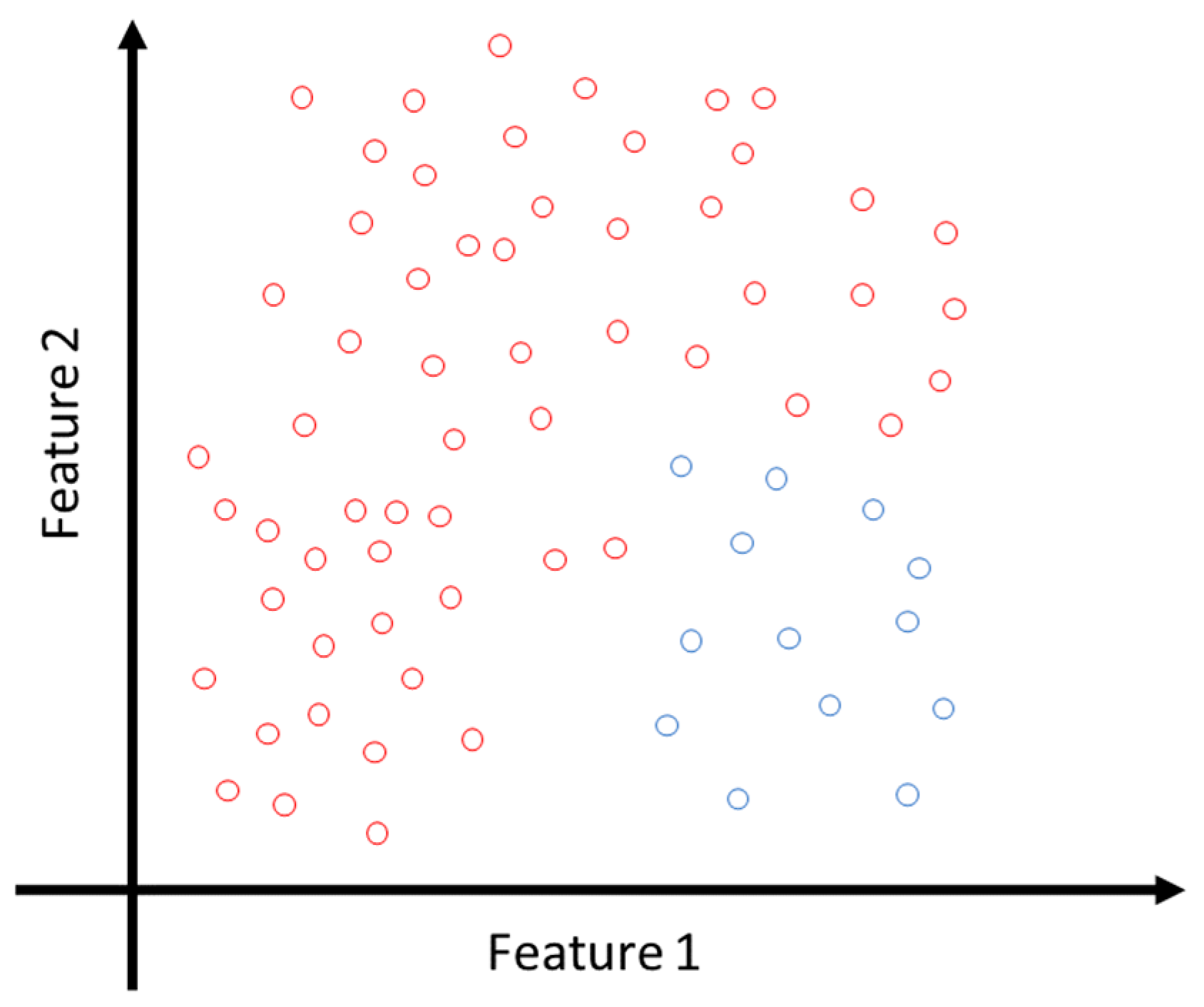
5]. This article uses the metrological data of imaging in the Jilin area provided by Jilin Provincial Metrological Bureau to build the fault sample. The fault sample dataset has seven features. However, in the image representation, in order to intuitively represent the unbalanced dataset, only two-dimensional images can be drawn here. The two-dimensional characteristics of positive and negative samples in the fault sample data are selected here, and the unbalanced two-dimensional dataset in two-dimensional coordinates is drawn in Figure 1, which shows the representation of an unbalanced 2D dataset in 2D coordinates.
For most datasets, there are two general ways to improve data balance: the oversampling method and the undersampling method. Oversampling is to repeat positive proportional data for categories with small sample numbers, and undersampling is to discard a portion of the data for sample species with a larger number of samples, thus making the number of samples under each category equal, such as with the K-nearest neighbor (KNN) algorithm and boosting algorithms [6]. Traditional oversampling techniques use random sampling, which simply copies the sample data to make the number of samples increase rapidly. This approach may cause overfitting problems: as the number of replicates of the samples increases, the error information in the samples will also be amplified, thus making the model in the learning process continue to fit the error information. The information learned from such models is too specific and insufficient, thus it will appear that the training set works well, but the test set works poorly [7]. In this paper, the SMOTE algorithm as improved based on the stochastic process is used. Its basic idea is to analyze the minority class samples and synthesize new samples via manual interpolation based on the characteristics of the minority class samples to increase the balance of the dataset. Figure 2 shows the process of a random selection of proximal points by using the SMOTE algorithm and the process of randomly generating new samples at the proximity point using the SMOTE algorithm.
Support vector machine theory first came from statistics as a binary linear classifier. In 1992, kernel methods were proposed by Bernhard E. Boser, Isabelle M. Guyon, and Vapnik. The introduction of kernel functions made support vector machine theory available for solving nonlinear classification problems [8].
Support vector machines are essentially binary classifiers, and when dealing with multiclassification problems, their algorithms must be improved. Currently, there are two methods for multiclassification using support vector machines: the direct method and the indirect method. The direct method directly modifies the objective function and combines the parameter solutions of multiple classification surfaces into one optimization problem and achieves multiclass classification by solving that optimization problem at once. This method is simple in principle but not easy to implement, and it is only applicable to small- and medium-sized problems and cannot be applied on a large scale. Indirect methods, i.e., constructing multiple binary solvers to transform a multiclassification problem into multiple binary problems, are more widely used, such as the one-vs-one method, the one-vs-all method, the derived directed acyclic graph method, and the binary tree method [9,10,11].
The one-vs-one method constructs a binary classifier in any two classes of training samples, and for the n -class classification problem, the one-vs-one method constructs C n 2 binary classifiers. The one-vs-all method treats each class of samples as one positive sample and the remaining samples as negative samples, thus for the n -class classification problem, the one-vs-all method must only construct n binary classifiers. Compared with the one-vs-one method, the computational effort of the one-vs-all method is much smaller than that of the one-vs-one method, but there are certain disadvantages of the one-vs-all method in solving the classification problem, such as the unbalanced number of positive and negative samples, the need to train all models when adding new categories or other elements, and the existence of some areas in which the samples within its range meet two or more hyperplane equations at the same time. Figure 3 show the classification schematics of the same set of two-dimensional data under the one-vs-one and one-vs-all methods, respectively. Under the premise of classification by using the one-vs-all method, there exist two classes of transition areas between hyperplanes [12,13]. For these areas, some discriminative methods are proposed, such as a “voting” scheme, in which the area is marked as the category with the highest number of points [14].
In the literature [15], a discrimination method for such transition areas was proposed: for sample points in a transition area, the class to which the sample belongs can be determined from the distance between the sample and two adjacent hyperplanes. Islam et al. concluded that in the transition area, the feature points belonging to the class are instead more distant than the hyperplanes of the class. This discriminative method, compared with the previous discriminative methods, no longer assigns the transition area to a certain class completely but divides it specifically according to the actual situation, which improves classification accuracy and precision to a certain extent. However, this method must discriminate each feature sample in the transition area in a targeted manner, and when the number of feature samples in the area is large or the number of sample classes is large, this method is not efficient. A one-time means is still needed to solve the problem.
Based on the method proposed in the literature [15], this paper proposes a CSH-SVM improvement algorithm that no longer calculates the distance between each sample located in the transition interval and the adjacent hyperplane. The transition interval is partitioned with the existing hyperplane equation to form a new hyperplane equation. Combined with the SMOTE algorithm to process the unbalanced samples, the four conditions of tower icing, conductor galloping, tower base settlement, and water corrosion are finally classified and predicted, and preventive measures can be taken when the tower has mechanical failure precursors. This improved algorithm has a faster response speed for the classification prediction of new samples because it no longer calculates the distance between samples and hyperplane frequently. On the premise of reducing the amount of calculation, it has better classification efficacy, which can well solve the problem of fault prediction and classification in practical engineering applications, thus improving the safety and service life of monitoring objects as well as reducing the loss of personnel and property.

2. Tower Mechanical Structure Modeling

The tilt sensor should be placed at the location where the displacement changes the most when the tower is deformed, and a finite element model of the tower must be constructed to achieve this purpose. First, the design modeler was used to modeling the mechanical structure of the tower, and the mechanical model was input to ANSYS Workbench platform for finite element analysis of the tower’s mechanical structure. Through the finite element analysis results, the placement position of the tilt sensor was analyzed to achieve the best monitoring effect [16].
Taking the MZ2-27 cathead linear tower as an example, the main material of the tower adopts angle steel as the material, the main material is Q345 steel, and the oblique material is Q235 steel. These relevant material parameters were imported into the design modeler, and the bolts were used to attach the main material and the oblique material, which can eliminate part of the stress generated by the tower vibration and reduce the shaking amplitude of the tower. Therefore, the tower cannot be regarded as a truss structure but should be simulated and analyzed as a mixed steel frame and truss structure. The parameters related to the main material and diagonal material are shown in Table 1.
Usually, the main material is regarded as a beam structure, which not only bears axial pressure and tension but also bends at a certain degree; the oblique material is regarded as a rod structure, which only bears axial strain and theoretically does not produce bending. Different from the classic ANSYS version, the Workbench platform set the line body as a beam element by default and eliminated the direct switch between beam element and rod element. Therefore, two solutions are proposed in this paper: one is to force the unit type of the oblique material to change to a Link180 unit through the command flow; the other is to use the beam unit instead of the rod unit and set the connection nodes on both sides of the beam unit to be hinged, releasing the rotation degrees of freedom in three directions to achieve accurate modeling. Because the oblique material of the tower generating a small bending moment is more realistic, and because the cross-sectional area of the line body must be recalculated if Method 1 is adopted, Method 2 was chosen for the mixed modeling of the truss and rigid frame.
The MZ2-27 cat-head-type linear tower is an overhanging tower. The force characteristic of the overhanging tower is that both sides of the conductor are not broken, thus the load of an overhanging tower is mainly composed of the wind load and ice load. Wind load includes line wind load, tower wind load, and insulator string wind load, and ice load mainly refers to the ice load of the conductor and the ground wire. In the Workbench platform, the stress of the tower under each working condition was calculated, and the load under each working condition was calculated by taking the wind speed of 10m/s and the conductor and ground wire’s icing thickness of 20mm as an example [17]. Relevant calculation formulas for line wind load, tower wind load, and insulator string wind load are provided in the literature [18].
The formula for calculating the line wind load is as follows:
W x = α · W o · μ z · μ sc · β c · d · L p · B 1 · sin 2 θ , W o = V 2 / 1600 ,
where W x is the standard value of horizontal wind load (kN) perpendicular to the wire and ground direction; α is the wind pressure unevenness coefficient; μ z is the wind pressure height variation coefficient; μ sc is the body coefficient of the conductor or ground; β c is the wind load adjustment coefficient of the conductor and ground of the 500 kV and 750 kV lines; d is the outer diameter of the conductor, ground, or the calculated outer diameter when icing (m); L p is the pole tower horizontal distance (m); B 1 is the guide, ground, and insulator string ice wind load increase factor; θ is the angle between the wind direction and the direction of the wire or ground (°); W o is the standard value of the base wind pressure (kN); V is the wind speed at the base height of 10 m (m/s).
The formula for calculating the wind load on the tower is as follows:
W s = W o · μ z · μ s · B 2 · A s · β z ,
where W s is the standard value of the tower wind load (kN); μ s is the body type coefficient of the member; B 2 is the increase coefficient of the wind load of the tower member over ice; A s is the calculated value of the projected area of the windward side member (m2); β z is the wind load adjustment coefficient of the tower.
The formula for calculating insulator string wind load is as follows:
W 1 = W o · μ z · B 1 · A 1 ,
where W 1 is the insulator string wind load standard value (kN); A 1 is the calculated value of insulator string bearing wind pressure area (m2).
The wire and ground wire ice loads are related to the maximum tension of the conductor and ground wire. The values of the conductor and ground wire ice load under a 20 mm icing degree are shown in Table 2 [19,20,21]. The calculation formula of the maximum tension of conductor and ground wire is as follows:
T max = F max · C nl k ,
where T max is the maximum tension of the wire and ground wire; F max is the calculated pull-off force of the wire and ground wire; k is the safety factor of the wire and ground wire; C nl is the new line coefficient, which is usually 0.95 in conservative calculations.
The MZ2-27 cat-head-type linear tower is an overhanging tower with bifurcated wire. The tower under a 20 mm icing degree carries 50% of the maximum tension of the conductor and 100% of the maximum tension of the ground wire.
The ice-covered load of the tower is the gross value of the wire icing load and ground wire icing load. Thus, the formula for the ice-covered load of the tower can be derived as follows:
W f = 0.95 ( F max 1 2 k 1 + F max 2 k 2 ) ,
where W f is the standard value of the ice load (kN); F max 1 is the calculated pull-off force of the wire (kN); k 1 is the safety coefficient of the wire; F max 2 is the calculated pull-off force of the ground wire (kN); k 2 is the safety coefficient of the ground wire.
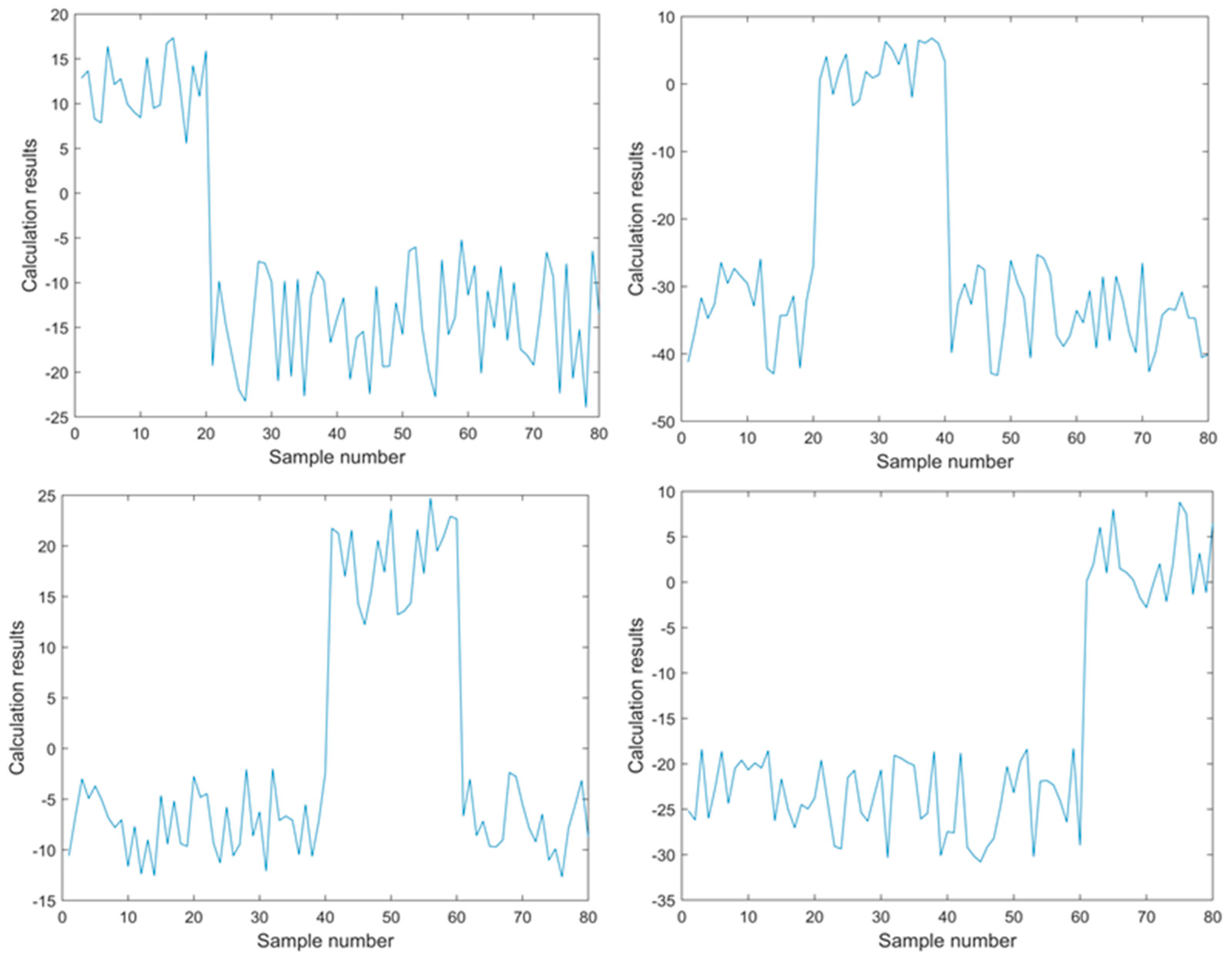
The results of the equivalent force analysis are shown in Figure 4. According to the calculation, the equivalent stress of the MZ2-27 cat-head type linear tower ranges from about 254.02 MPa to 317.52 Mpa, the maximum displacement point is 18.4 mm, and the height of the point is 9.63 m from the main rod of the tower to the ground when the wind speed is 10 m/s and the ice coating thickness of the conductor and ground wire is 20 mm. For the MZ2-27 cat-head type linear tower, a trigonometric function is needed to calculate the angle change of the monitoring point at a specific height. The included angle between the tower’s main material and the horizontal ground is about 77.42°, and the sine value of the included angle is 0.976. Combined with the distance between the tower foot and the monitoring point in the direction of the main material, the angle of the monitoring point at a specific height can be inversely calculated. The resulting angular deflection and the height at which the point is located meet the following equation:
θ = 2 sin 1 0.976 s h ,
where θ is the size of the angle change; s is the size of the displacement of the point (m); h is the height of the point (m). Therefore, when the wind speed of the tower is 10 m/s and the ice coating thickness of the conductor and ground wire is 20 mm, the angle change at 9.63 m from the tower foot is about 0.214°.

3. Construction of Tower Mechanical Failure Dataset Based on SMOTE Algorithm

In the process of the long-term monitoring of towers, it was found that the original dataset composed of fault information has the following characteristics: the number of samples generated by normal operation of towers is much larger than the number of samples where faults occur, the frequency of occurrence of various types of mechanical faults is different, and it is impossible to artificially control the number of samples generated by each type of fault, resulting in a poorly balanced dataset which is difficult to use directly in the machine learning process. Thus, the SMOTE algorithm was chosen to process the original dataset [22]. There are three steps in the process of implementing the SMOTE algorithm. First, the known sample points were edited to remove the points that do not play a significant role in the classification process to avoid computational overload during the subsequent process. Then, the KNN algorithm was used to select the K similar sample points that are closest to the sample point x i . Last, M sample points x jn ( n = [ 1 , 2 , M ] ) were randomly selected among the K similar sample points. In practice, the value of M was usually taken as 5, which ensured that the operation was not too large while at the same time making the sample points grow quickly. M sample points were linked to the original sample point x i , and any point during the period was taken as the new sample point x N . The new sample points were constructed according to the SMOTE random formula, where ξ is a random number from 0 to 1 [23]. Repeating this process under this condition, any number of sample points corresponding to the category can be obtained.
x N = x i + ξ ( x jn x i )   ξ ( 0 , 1 ) ,
The SmoteOverSampling function was required for processing the dataset using the SMOTE algorithm, and the Vienna development method (VDM) algorithm was referenced in this function to calculate the nominal attribute distances [24]. In the SmoteOverSampling function, the parameters that can be adjusted are C, k, and type. The parameter C is the cost vector, which refers to the size of the cost of a sample being misclassified to another class in the classification problem. Adjusting the parameter C controls the proportion of each class in the new dataset processed with the SMOTE algorithm. In this paper, the ratio of positive class to negative class samples should be controlled as 1:1, thus the parameter C should take the value of [1, 1]. The introduced KNN algorithm must introduce the parameter k, which indicates that the value is taken for the k proximity sample points around each known sample point. In the general case, the parameter k value was taken as 5. In the parameter type, two options, nominal or numeric, are available. Under nominal, the SMOTE algorithm uses VDM to process the nominal attributes to calculate the distance, and under numeric, the SMOTE algorithm uses Euclidean distance to process the nominal attributes. Thus, the nominal option was chosen as the value of the parameter type [25]. Processing the dataset with the SMOTE algorithm helped to improve classification accuracy. Figure 5 shows the comparison results of some data in the fault sample data under two-dimensional characteristics before and after processing. In the preprocessing dataset, each sample contained two features, and the ratio of positive to negative samples is 20:100. The new dataset increased the number of positive samples with the same number of negative samples, making the ratio of positive to negative samples achieve 100:100.
The original dataset and the new dataset were validated separately using LibSVM. In the validation process, the proportion of test samples was 30% of all samples, and the number of the test samples of the original dataset was 36, among which the number of positive samples was 6 and the number of negative samples was 30. The number of test samples of the new dataset after SMOTE algorithm processing was 60, among which the number of both positive and negative samples was 30. Without normalization, as shown in Figure 6, the validation accuracy of the original dataset was 88.89%, and misclassification occurred four times, all of which occurred in the positive samples. As shown in Figure 7, the validation accuracy of the new dataset was 91.67% and misclassification occurred five times. It is concluded that in unbalanced samples, the classifier is more likely to classify the samples to the side with a larger number, and the dataset obtained with the SMOTE algorithm is better balanced and has higher prediction accuracy.
In practice, due to the randomness of the SMOTE algorithm, it leads to the problem that the generated new samples and the original samples will overlap or nearly overlap, especially in a dataset with a small number of features. At this time, the number of effective samples that really work is still lower than the actual number of samples, thus in low-dimensional data, the value of parameter C should be changed appropriately so that the number of new samples of a certain category is slightly larger than the expected number, which can eliminate the influence of duplicate samples on the classification results to some extent and compensate for the number of effective samples to some extent.

4. CSH-SVM Classification Algorithm

4.1. Principle of Multiclassification SVM Classification

In linear separable problems, we can find the optimal hyperplane to separate two classes of points. The optimal hyperplane can be expressed as:
ω T x + b = 0 ,
The two types of points in space can be expressed as:
{ ω T x i + b 0                         y i = + 1 ω T x i + b 0                         y i = 1 ,
Applying the constraint y i ( ω x i + b ) 1 , the objective function was obtained and is as follows:
min 1 2 ω 2 ,
The Lagrange multiplier method was used to solve the objective function as below:
L ( ω , b , α ) = 1 2 ω 2 i = 1 n α i [ y i ( ω T x + b ) 1 ] , α = { α 1 , , α n } ,
For the objective ω ,   b for partial derivatives, the maximum problem was converted into a minimum problem by using pairwise problems. Because of the inequal relationship in the constraints, the Lagrange multipliers must meet the Karush-Kuhn-Tucker condition. The final solution to the equation is:
min α 1 2 i = 1 n j = 1 n α i α j y i y j ( x i · x j ) i = 1 n α i ,
The solution must also must meet the following constraints: { i = 1 n α i y i = 0 α i 0 .
In solving practical problems, it is usually necessary to introduce a relaxation factor, thus the constraint becomes:
y i ( ω x i + b ) 1 ξ i ,
Under the new constraints, the new objective function is:
min 1 2 || ω || 2 + C i = 1 n ξ i ,
By solving the objective function, we can find the optimal hyperplane that separates the two classes of points, and it is this property that determines the performance of support vector machine theory in binary classification problems over other machine learning methods. However, for multiclassification problems, SVMs generally must construct multiple binary classifiers, thus the multiclassification problem of SVMs should be viewed as multiple binary classification problems to solve, i.e., the hyperplane should be repeatedly constructed to meet the requirements of multiclassification.

4.2. CSH-SVM Improvement Algorithm

Based on the method proposed in the literature [15], when a sample satisfies multiple hyperplanes at the same time, it can be sorted by the distance between the sample and the hyperplane, as shown in Figure 8. This process can find which distance between the sample point and its actual category under the hyperplane is the maximum to be considered part of that category. This method is targeted to special samples without changing the SVM model, which is difficult to realize in practical production and application. In this paper, this was improved by finding a new hyperplane to divide the transition area by the original hyperplane. In the high-dimensional space, any two hyperplanes must intersect and produce an angle. It is because these angles exist that some samples meet the hyperplane equations on both sides at the same time. By finding the central partition in the two hyperplanes, we can accurately determine the specific category to which the sample belongs, as shown in Figure 8.
Take the three-dimensional data as an example: the intersection of two hyperplanes must produce an angle, and there is a certain connection between the angle of the two planes and the normal vectors of the two planes, as shown in Figure 9. The two hyperplane equations are as follows:
OH 1 : ω 1 T x + b 1 = 0 ,
OH 2 : ω 2 T x + b 2 = 0 ,
By the definition of a hyperplane, ω 1 and ω 2 are the normal vectors of the two original hyperplanes O H 1 and O H 2 . The angle formed by the intersection of ω 1 and ω 2 is θ , which is the same as the angle formed by the two hyperplanes O H 1 and O H 2 . When 0 > θ π 2 , the intersection of ω 1 and ω 2 gives ω 1 || ω 1 || and ω 2 || ω 2 || when the two vectors have the same length and the same direction as ω 1 and ω 2 . ω 1 || ω 1 || and ω 2 || ω 2 || The angle parallels of the two vectors in the plane where they are located are perpendicular to the improved hyperplane O H 12 , thus ω 1 || ω 1 || and ω 2 || ω 2 || are added to the vector ω 12 , which is the normal vector of the improved hyperplane O H 12 .
ω 12 = ω 1 || ω 1 || + ω 2 || ω 2 || ,
When π 2 > θ 0 , ω 1 || ω 1 || and ω 2 || ω 2 || in the plane of the two vectors’ angle bisection are parallel to the improved hyperplane
, the size of the angle formed by the two planes should be complementary to the two vectors’ angle. Thus, the improved hyperplane O H 12 normal vector ω 12 and ω 1 and ω 2 can be obtained by calculating the relationship as follows:
ω 12 = ω 1 || ω 1 || ω 2 || ω 2 || ,
The improved hyperplane O H 12 has a common solution X 0 with the hyperplanes O H 1 and O H 2 , and X 0 is a nonzero vector with the same characteristic dimension. The solution of X 0 by the original hyperplane equations O H 1 and O H 2 is as follows:
X 0 = b 2 b 1 ( ω 1 ω 2 ) T
An improved construction of the hyperplane equation of O H 12 is as follows:
O H 12 : ω 12 T x + b 12 = 0
X 0 is a special solution of the improved hyperplane equation O H 12 , which can be obtained by substituting the following into Equation (19):
b 12 = ( b 2 b 1 ) ( ω 12 ω 1 ω 2 )

4.3. Validation Results

The multicategory support vector machine substituted each sample datum in the dataset into each hyperplane equation separately, and the classes considered as positive samples had significantly different results in their corresponding hyperplane equations. Taking the original hyperplane as an example, when solving the hyperplane equation O H 1 , the samples marked as the first category were regarded as positive samples, and the samples marked as other categories were regarded as negative samples. Thus, when the first category is substituted into the hyperplane equation O H 1 , the computed results should be positive and the computed results of the other categories should be negative. In order to verify the accuracy of the CSH-SVM improvement algorithm, we randomly selected 20 samples from each class in the tower dataset to form a validation dataset with a total of 80 samples, and Figure 10 shows the results of validating the four classes of samples in the corresponding hyperplane equation. This process simulates the model-building process of SVM in multiclassification scenarios, and the calculated values obtained through this process can intuitively compare the classification performance of SVM between scenarios. It can be found in Figure 10 that the resulting values obtained from the samples of the corresponding categories under the hyperplane equations of those categories were significantly different from those of the other categories.
Using the CSH-SVM improvement algorithm, the resulting values obtained for the four classes of samples in the corresponding hyperplane equations are shown in Figure 11.
From the data in Figure 11, it is clear that even though the calculation results of the improved hyperplane for the samples were different from those of the original hyperplane, the classification results are consistent. The calculation results of the first category of labeled data are clearly different from the other categories. By observation, it was found that the calculation results of the two hyperplanes had opposite trends with the samples. The calculated result values that were larger in the original hyperplane O H 1 became smaller in the improved hyperplane O H 23 instead. Thus, the images in the two figures, which have almost the same shape, change in the exact opposite trend.
In order to purposefully compare the classification performance of the two hyperplanes for the transition area, two support vector machines were used to classify the actual operational data of the towers separately, and a total of 1500 test samples from the four types were selected out of 6000 samples. Among them, 77 samples were misclassified at least once. In order to make the images easy to observe, the samples that were correctly classified twice are ignored, and only the classification results of the 77 samples that were misclassified are plotted. Figure 12 and Figure 13 show the classification results of the one-vs-all classification SVM and CSH-SVM, respectively.
By comparison, the improved CSH-SVM algorithm had higher accuracy for the multiclassification problem, with 15 out of 77 samples correctly classified to the corresponding class with the new hyperplane. The quadratic planning prediction for these 15 samples shows that all such samples existed in the transition area. The classification accuracy was 94.87% before the improvement and 95.87% after the improvement. It is concluded that this improved algorithm has no effect on the sample points that exist in well-defined areas, whereas it can improve the classification accuracy for sample points existing in unspecified areas, making the results of the one-vs-all classification problem more accurate.

5. Conclusions

When the SMOTE algorithm and the improved CSH-SVM algorithm were applied at the same time, the classification effect was further improved: of the 6000 samples that are not uniformly extracted from the tower fault dataset, only 63 samples had errors, and the accuracy rate was 98.95%. This shows that the method proposed in this study is well-suited for the specific application scenario of tower fault classification. Figure 14 shows the SMOTE and CSH-SVM improved algorithm classification results.
In this paper, a tower mechanical fault classification method based on the SMOTE algorithm and an improved CSH-SVM algorithm is proposed for monitoring the tower operation status and the stability of the mechanical structure. ANSYS Workbench was used to model the tower mechanical structure and analyze the sensor placement position and accuracy requirements. The tower operation data was processed using the SMOTE algorithm to make its data features suitable for machine learning and to obtain better classification results. The improved CSH-SVM algorithm was applied to classify and predict tower faults; it improved the potential problems of one-vs-all classification methods for the classification of samples in the transition area and the accuracy of classification and prediction of samples in the transition interval, and it thus provides a guarantee of safety in the transmission process of towers. Compared with the method in the literature [15], the improved CSH-SVM algorithm does not need to calculate the distance from the sample point to the hyperplane frequently, which reduces the amount of calculation in the prediction process. Moreover, the application of the SMOTE algorithm has a good balance for the tower fault dataset targeted by this study. Compared with the existing traditional monitoring methods, the prediction results were more accurate and were calculated faster, especially in the classification process of unbalanced datasets. However, this study also had certain limitations. When the dataset itself is highly balanced, the improvement effect was smaller than that of the unbalanced dataset. Therefore, when applying this method, it should be inclined to classify and predict the unbalanced dataset to achieve the best classification effect.

6. Patents

This manuscript has produced four Chinese patents, namely:
Changchun Power Supply Company of State Grid Jilin Electric Power Co., Ltd., and Changchun University of Technology. “A big data based online monitoring system and method for transmission line tower posture.” Patent No.: CN114719909A. Authorization time: 8 July 2022.
Changchun Power Supply Company of State Grid Jilin Electric Power Co., Ltd., and Changchun University of Technology. “A method for predicting icing galloping of overhead transmission lines based on multi-information fusion.” Patent No.: CN114676540A. Authorization time: 28 June 2022.
Changchun Power Supply Company of State Grid Jilin Electric Power Co., Ltd., and Changchun University of Technology. “Wind power supply system blade deformation detection circuit.” Patent No.: CN216922368U. Authorization time: 8 July 2022.
Changchun Power Supply Company of State Grid Jilin Electric Power Co., Ltd., and Changchun University of Technology. “Online monitoring circuit of transmission tower state based on the Internet of Things.” Patent No.: CN216927421U. Authorization time: 8 July 2022.

Author Contributions

Conceptualization, H.W. (Heran Wang) and H.Y.; methodology, S.H.; software, H.W. (Heran Wang); validation, H.W. (Heran Wang) and H.Y.; investigation, S.H. and X.H.; writing—original draft preparation, H.W. (Heran Wang); writing—review and editing, S.H. and H.W. (Hanye Wu); supervision, S.H. and X.H. All authors have read and agreed to the published version of the manuscript.

Funding

This research was funded by the State Grid Jilin Electric Power Co., Ltd. Changchun Power Supply Company, funding number SGJLCC00KJJS2100825. The APC was funded by the State Grid Jilin Electric Power Co., Ltd. Changchun Power Supply Company.

Data Availability Statement

The meteorological data of icing in the Jilin area supporting this paper are from the Jilin Provincial Meteorological Bureau.

Acknowledgments

The authors would like to thank the State Grid Jilin Electric Power Co., Ltd. Changchun Power Supply Company for providing the research object of this article. We would also like to thank Xu for his enthusiastic provision and arrangement of the experimental objects and the experimental environment mentioned in the article.

Conflicts of Interest

The authors declare no conflict of interest. The funders had no role in the design of the study, nor in the collection, analyses, or interpretation of data, nor in the writing of the manuscript, nor in the decision to publish the results.

References

  1. Ji, H.T.; Liu, J.F. Operation Status Monitoring of Transmission Tower in Power System based on Data Fusion. Int. J. Circuits Syst. Signal Process. 2022, 16, 543–550. [Google Scholar] [CrossRef]
  2. Huang, X.B.; Liao, M.J.; Xu, G.H.; Zhu, Y.C.; Zhao, L. Stress Monitoring Method for Transmission Line Towers Using Fiber Grating Sensors. Power Autom. Equip. 2016, 36, 68–72. (In Chinese) [Google Scholar] [CrossRef]
  3. Xiong, Y.J.; Huang, S.; Yang, Y.; Liu, Y.; Liu, M.R.; Deng, X. Design and implementation of monitoring equipment for tilt deformation of Beidou Tower. J. Chang. Univ. 2021, 35, 15–19. (In Chinese) [Google Scholar]
  4. Liu, Y.C.; Chen, Y.; Paul, P.; Fan, S.H.; Ma, X.M.; Zhang, G.X. A Review of Power System Fault Diagnosis with Spiking Neural P Systems. Appl. Sci. 2021, 11, 4376. [Google Scholar] [CrossRef]
  5. Yu, W.H.; Chen, J.X.; Wei, C. A hierarchical learning model for inferring the labels of points of interest with unbalanced data distribution. Int. J. Appl. Earth Obs. Geoinf. 2022, 108, 102751. [Google Scholar] [CrossRef]
  6. Li, X.Q.; Jiang, H.K.; Liu, S.W.; Zhang, J.J.; Xu, J. A unified framework incorporating predictive generative denoising autoencoder and deep coral network for rolling bearing fault diagnosis with unbalanced data. Measurement 2021, 178, 109345. [Google Scholar] [CrossRef]
  7. Shi, Q.; Zhang, H. Fault diagnosis of an autonomous vehicle with an improved SVM algorithm subject to unbalanced datasets. IEEE Trans. Ind. Electron. 2020, 68, 6248–6256. [Google Scholar] [CrossRef]
  8. Zhou, J.B.; Xiao, M.H.; Niu, Y.; Ji, G.J. Rolling Bearing Fault Diagnosis Based on WGWOA-VMD-SVM. Sensors 2022, 22, 6281. [Google Scholar] [CrossRef]
  9. Otchere, D.A.; Ganat, T.O.A.; Gholami, R.; Ridha, S. Application of supervised machine learning paradigms in the prediction of petroleum reservoir properties: Comparative analysis of ANN and SVM models. J. Pet. Sci. Eng. 2021, 200, 108182. [Google Scholar] [CrossRef]
  10. Vos, K.; Peng, Z.X.; Jenkins, C.; Shahriar, M.R.; Borghesani, P.; Wang, W.Y. Vibration-based anomaly detection using LSTM/SVM approaches. Mech. Syst. Signal Process. 2022, 169, 108752. [Google Scholar] [CrossRef]
  11. Le, T.C.; Nguyen, T.N.; Khatir, S.; Nguyen, P.T.; Mirjalili, S.; Nguyen, K.D. An efficient approach for damage identification based on improved machine learning using PSO-SVM. Eng. Comput. 2022, 38, 3069–3084. [Google Scholar] [CrossRef]
  12. Chauhan, V.K.; Dahiya, K.; Sharma, A. Problem formulations and solvers in linear SVM: A review. Artif. Intell. Rev. 2019, 52, 803–855. [Google Scholar] [CrossRef]
  13. Da Wang, S.; Xu, B.; Zhu, Z.H.; Li, J.; Lu, J.Y. Reliability Analysis of Concrete Gravity Dams Based on Least Squares Support Vector Machines with an Improved Particle Swarm Optimization Algorithm. Appl. Sci. 2022, 12, 12315. [Google Scholar] [CrossRef]
  14. Zhang, X.J.; Zhang, M.; Xiang, Z.Y.; Mo, J.L. Research on diagnosis algorithm of mechanical equipment brake friction fault based on MCNN-SVM. Measurement 2021, 186, 110065. [Google Scholar] [CrossRef]
  15. Islam, M.M.M.; Kim, J.M. Reliable multiple combined fault diagnosis of bearings using heterogeneous feature models and multiclass support vector Machines. Reliab. Eng. Syst. Saf. 2019, 184, 55–66. [Google Scholar] [CrossRef]
  16. Li, Y.Z.; Dai, W.; Huang, T.T.; Zhang, W.F. Adaptive Early Warning Method Based on Similar Proportion and Probability Model. Appl. Sci. 2020, 10, 4278. [Google Scholar] [CrossRef]
  17. Huang, X.B.; Zhao, L.; Chen, Z.L.; Liu, C. An online monitoring technology of tower foundation deformation of transmission lines. Struct. Health Monit. 2019, 18, 949–962. [Google Scholar] [CrossRef]
  18. Electric Power Planning and Design Institute. Technical Regulation for Structural Design of Overhead Transmission Line Poles and Towers; DL/T 5154-2012; National Energy Administration: Beijing, China, 2012. (In Chinese)
  19. Guo, C.X.; Wang, B.; Wu, Z.Y.; Ren, M.; He, Y.F.; Albarracín, R.; Dong, M. Transformer failure diagnosis using fuzzy association rule mining combined with case-based reasoning. IET Gener. Transm. Distrib. 2020, 14, 2202–2208. [Google Scholar] [CrossRef]
  20. Shao, Y.; Yuan, X.F.; Zhang, C.J.; Song, Y.; Xu, Q.Y. A Novel Fault Diagnosis Algorithm for Rolling Bearings Based on One-Dimensional Convolutional Neural Network and INPSO-SVM. Appl. Sci. 2020, 10, 4303. [Google Scholar] [CrossRef]
  21. Bhowmik, C.; Chakraborti, P. Analytical and experimental modal analysis of electrical transmission tower to study the dynamic characteristics and behaviors. KSCE J. Civ. Eng. 2020, 24, 931–942. [Google Scholar] [CrossRef]
  22. Zhang, Y.; Liu, Q. On IoT intrusion detection based on data augmentation for enhancing learning on unbalanced samples. Future Gener. Comput. Syst. 2022, 133, 213–227. [Google Scholar] [CrossRef]
  23. Kaur, H.; Pannu, H.S.; Malhi, A.K. A systematic review on imbalanced data challenges in machine learning: Applications and solutions. ACM Comput. Surv. (CSUR) 2019, 52, 1–36. [Google Scholar] [CrossRef] [Green Version]
  24. Wang, L.; Han, M.; Li, X.J.; Zhang, N.; Cheng, H.D. Review of classification methods on unbalanced data sets. IEEE Access 2021, 9, 64606–64628. [Google Scholar] [CrossRef]
  25. Zhao, C.; Sun, J.L.; Lin, S.L.; Peng, Y. Fault Diagnosis Method for Rolling Mill Multi Row Bearings Based on AMVMD-MC1DCNN under Unbalanced Dataset. Sensors 2021, 21, 5494. [Google Scholar] [CrossRef]
Figure 1. The representation of an unbalanced 2D dataset in 2D coordinates.
Applsci 13 01331 g001
Figure 2. (a) SMOTE algorithm random selection process; (b) SMOTE algorithm random generation process.
Applsci 13 01331 g002
Figure 3. (a) One-vs-one method of classifying hyperplanes; (b) one-vs-all method of classifying hyperplanes.
Applsci 13 01331 g003
Figure 4. Equivalent force analysis results.
Applsci 13 01331 g004
Figure 5. (a) Comparison of echocardiogram dataset before applying SMOTE algorithm; (b) comparison of echocardiogram dataset after applying SMOTE algorithm.
Applsci 13 01331 g005
Figure 6. Echocardiogram raw dataset validation accuracy.
Applsci 13 01331 g006
Figure 7. SMOTE echocardiogram dataset validated accurately.
Applsci 13 01331 g007
Figure 8. (a) Relationship between samples in the transition area and the corresponding category hyperplane; (b) Relationship between the improved hyperplane and the corresponding category samples.
Applsci 13 01331 g008
Figure 9. Schemes follow the same formatting.
Applsci 13 01331 g009
Figure 10. Calculated results of four types of samples under the original hyperplane.
Applsci 13 01331 g010
Figure 11. Calculation results of four types of samples under improved hyperplane.
Applsci 13 01331 g011
Figure 12. Classification results of misclassified samples in one-vs-all classification SVM.
Applsci 13 01331 g012
Figure 13. Classification results of improved CSH-SVM algorithm.
Applsci 13 01331 g013
Figure 14. SMOTE and CSH-SVM improved algorithm classification results.
Applsci 13 01331 g014
Table 1. Tower main material and slant material related parameters.
Component NameMaterial TypeDensity (g/cm3)Young’s Modulus (G∙Pa)Poisson’s RatioYield Strength (MPa)
Main MaterialsQ345 steel7.852060.3345
Slanting materialQ235 steel235
Table 2. Icing degree of 20 mm under the guide, ground wire ice load percentage value table (%).
Tower TypeSingle WireBifurcated WireDouble Split Above WireGround Wire
Overhanging type505045100
Tensile type1007070100
Disclaimer/Publisher’s Note: The statements, opinions and data contained in all publications are solely those of the individual author(s) and contributor(s) and not of MDPI and/or the editor(s). MDPI and/or the editor(s) disclaim responsibility for any injury to people or property resulting from any ideas, methods, instructions or products referred to in the content.

