An Experimental Setup to Detect the Crack Fault of Asymmetric Rotors Based on a Deep Learning Method

Abstract

Crack is a common fault of rotor systems. The research on crack fault detection methods is mainly divided into numerical and experimental studies. In numerical research, the current fault detection algorithms based on deep learning are mostly applied to bearings and gearboxes, and there are few studies on rotor fault diagnosis. In experimental research, the rotors used in an experiment are mostly single-span rotors. However, there are complex structures such as multi-span rotor systems in the actual industrial field. Thus, the fault detection algorithms that have been successfully applied on single-span rotors have not been verified on complex rotor systems. To obtain a fault signal close to the actual asymmetric shaft system of an asymmetric rotor system and validate the fault detection method, the crack fault detection platform is designed and built independently. We measure the vibration signals of three channels under five working conditions and establish an intelligent detection method for crack location based on a residual network. The factors that influence fault detection performance are analyzed, and the influence laws are discussed. Results show that the accuracy and anti-noise performance of the proposed method are higher than those of the commonly used machine learning. The average accuracy is 100% when SNR (signal-to-noise ratio) is greater than or equal to −2 dB, and the average accuracy is 98.2% when SNR is −4 dB.

1. Introduction

Fault detection is an important branch in rotor dynamics and has attracted extensive attention from many scholars. A lot of research on dynamic characteristics analysis and uncertainty quantification of faulty rotor systems has been conducted by many domestic and international scholars. The main purpose is to deepen understanding of faulty rotor systems and provide a theoretical basis and technical support for rotor fault detection in different environments. Cracks are common faults in rotor systems. If a crack is not found in time, it will expand deeper, resulting in excessive rotor vibration, affecting the safe operation of the unit, and it may cause casualties in serious cases. Therefore, it is necessary to study crack rotor fault detection method.

The research on crack fault detection methods is mainly divided into numerical and experimental studies. It is an economical and feasible idea to establish a numerical model to study crack fault detection methods based on numerical signals. In 2002, Bachschmid et al. [1] proposed a multi-rotor fault detection method based on a numerical model. The fault parameters were detected by the least square method for multi-order harmonic components, and a residual map was introduced to strengthen the visualization process. In 2004, Friswell et al. [2] proposed a numerical model-based fault detection approach for cracked rotors. The modal expansion method was used to map the response at the finite measuring point to the whole model. Then, the equivalent fault force and torque were calculated. The fault parameters were detected based on the least square method. In 2004, Sekhar et al. [3] used a method based on a numerical model to diagnose the location and depth of rotor cracks and used the least square method to achieve the best matching of fault parameters in the time domain. The diagnostic effect of this method was verified by numerical simulation signals. The influence of the number of measuring points, bearing calibration deviation and model error on the diagnostic accuracy was also studied. Subsequently, Sekhar et al. [4] detected the location and depth of double crack faults on the rotor by numerical signals. In the same year, Chen et al. [5] adopted the wavelet finite element method to establish three curves with the first three vibration frequencies of the crack shaft as input, and the crack location and depth were diagnosed according to the intersection of the curves. In 2008, Babu et al. [6] proposed a crack diagnosis technology based on an amplitude deviation curve by extracting the axial amplitude and slope of the cracked rotor and completed the crack location identification in a double-cracked rotor. In 2013, Varney et al. [7] used numerical methods to analyze the response characteristics of cracked rotors and pointed out that the fault parameters of rotor cracks could be estimated by using the second harmonic components of the system. Finally, the estimation values of crack location and depth were given. In 2014, Haji et al. [8] proposed a rotor crack fault detection method based on orthogonal natural frequency. In this method, the extracted features have sharp notch peaks at the crack location rather than circular peaks at the crack location. According to different peak shapes, crack fault detection can be realized. In 2016, Soeffker et al. [9] proposed a crack fault detection method based on numerical signals by combining support vector machine and wavelet analysis. The research results show that this method has stronger robustness and can effectively deal with interference and noise. In 2020, Gupta et al. [10] generated the vibration signals of the rotor system under unbalanced force and crack fault by a numerical method, built an artificial neural network, and realized the classification of unbalanced faults and crack faults. In 2020, Sathujoda et al. [11] used the finite element method (FEM) to simulate the transient response of a slant cracked rotor during shutdown. The crack location detection was realized by transforming the basic vibration mode into the wavelet space.

Experimental research is the most direct verification method for fault detection, and it is also an important step before the fault detection algorithm is applied to the actual industrial field. In 2000, Bachschmid et al. [12] used the fault detection method based on a numerical model to diagnose the crack location and depth and verified it on an experimental platform. In this study, the location information was obtained by the least square method in the frequency domain, and the depth information was obtained by the ratio of equivalent bending moment and static bending moment. In 2005, Pennacchi et al. [13] proposed a crack location detection method based on a numerical model in the frequency domain. The location diagnosis of shallow cracks and deep cracks was carried out on a large experimental platform. In 2006, Yao et al. [14] used a fault detection method based on a numerical model to detect crack existence and location in a rotor system with both rub-impact and crack faults and carried out experimental verification. In 2009, Dong et al. [15] used the empirical mode decomposition (EMD) method to decompose a non-coupled signal and used Laplace wavelet to extract the modal parameters, detected the crack location and depth, and carried out experiments to verify the method.

The above literature review, shows that the research algorithms mainly include model-based and signal-based detection algorithms. The application requires a strong theoretical level, different research requires different algorithms, and there is still a certain distance from the actual industrial field application. Although most rotors used in the experiment are single-span rotors, there may be complex structures such as multi-span rotor systems in the actual industrial field. For example, generator rotors and cracks will bring high-order harmonic vibration to the shafting, will easily lead to subcritical resonance peaks and increase the risk of resonance of the system. Therefore, studying the fault detection method of asymmetric shafting with cracks and detecting the location of cracks has great scientific research value and practical application value.

In order to overcome the problem that traditional fault diagnosis algorithms rely on artificial experience, some scholars have gradually adopted a deep learning algorithm to study the fault diagnosis method, among which the convolutional neural network (CNN) has received the most attention. In 2016, Janssens et al. [16] first applied CNN to gearbox fault classification. Compared with the traditional artificial feature extraction machine learning method, the accuracy rate increased by about 6%. Zhang et al. [17,18] studied bearing fault transfer learning under different working conditions based on a convolution neural network and a transfer learning method, which have better adaptability than traditional methods. Yuan et al. [19] realized rotor fault classification based on a convolution neural network and multi-source data. In the fault diagnosis experiment of a rotor system, the accuracy rate reached 98.97%. Han et al. [20] adopted a domain adaptive method of joint adaptive distribution to study the problem of fault transfer diagnosis on the three data sets of fan, bearing and gearbox and verified the applicability of the proposed method. Yang et al. [21] adopted a multi-scale domain adaptive method to study the transfer of bearing experimental fault data to real bearing fault data for diagnosis, which achieved higher accuracy than the traditional method. Wen et al. [22] proposed a new transfer diagnosis method combining sparse autoencoder and transfer learning methods and tested it on a bearing data set. Compared with the traditional algorithm, the accuracy reached 99.82%. Wang et al. [23] proposed a new transfer diagnosis method by combining a residual network and local adaptation and studied the domain adaptation between different bearing fault data sets. Ren et al. [24] considered the problem of fault diagnosis without a large number of fault samples and proposed a model based on autoencoder and capsule network, which was tested on a bearing data set and achieved nearly 100% diagnostic accuracy. Zhang et al. [25] studied the bearing fault detection problem under small samples by using the Siamese neural network. Compared with traditional methods, they achieved the highest accuracy in small sample fault diagnosis. Zhu et al. [26] combined the symmetrized dot pattern image and convolutional neural network method to classify rotor faults. Gao et al. [27] solved the problem of data enhancement by combining FEM and generative adversarial networks (GAN) and verified it on rotor fault classification data. Lei et al. [28] and Nath et al. [29] reviewed the application of deep learning in rotating machinery and pointed out the shortcomings and development direction of current research. In addition, Sun et al. [30,31] introduced an Internet of Things system that provides new ideas for solving industrial big data and fault diagnosis. At the same time, Yuan et al. [32,33]. studied the fault diagnosis method based on thermal imaging technology and deep learning. Different from the above fault diagnosis using time series vibration data, this method uses thermal imaging technology to collect fault data, which is an economical nondestructive testing technique. The fault detection method based on deep learning mainly extracts the high-dimensional features of fault signals through autonomous learning and then carries out fault classification or quantitative detection. The deep learning method can overcome the background noise of the actual industrial site, and the training process and recognition process of the model do not require too much human participation, so it has low requirements for the theoretical foundation of the actual operators.

Based on the above research background, we found that the existing fault diagnosis methods based on deep learning mainly focus on bearings and gearboxes, and there is a lack of research on rotors, especially asymmetric cracked rotors. In order to realize the crack fault detection of asymmetric shaft systems, we design and independently build an experimental platform for crack fault detection of asymmetric shaft system in this paper. The intelligent detection method of crack fault detection based on experimental signals is studied. The rest of the paper is organized as follows: The proposed methodology will be introduced in Section 2. In Section 3, the experimental platform of asymmetric shaft crack fault detection is introduced. Then, Section 4 analyzes the performance of the adopted method on the data set collected by the experimental platform in detail. Finally, Section 5 gives a summary.

2. Fault Detection Method

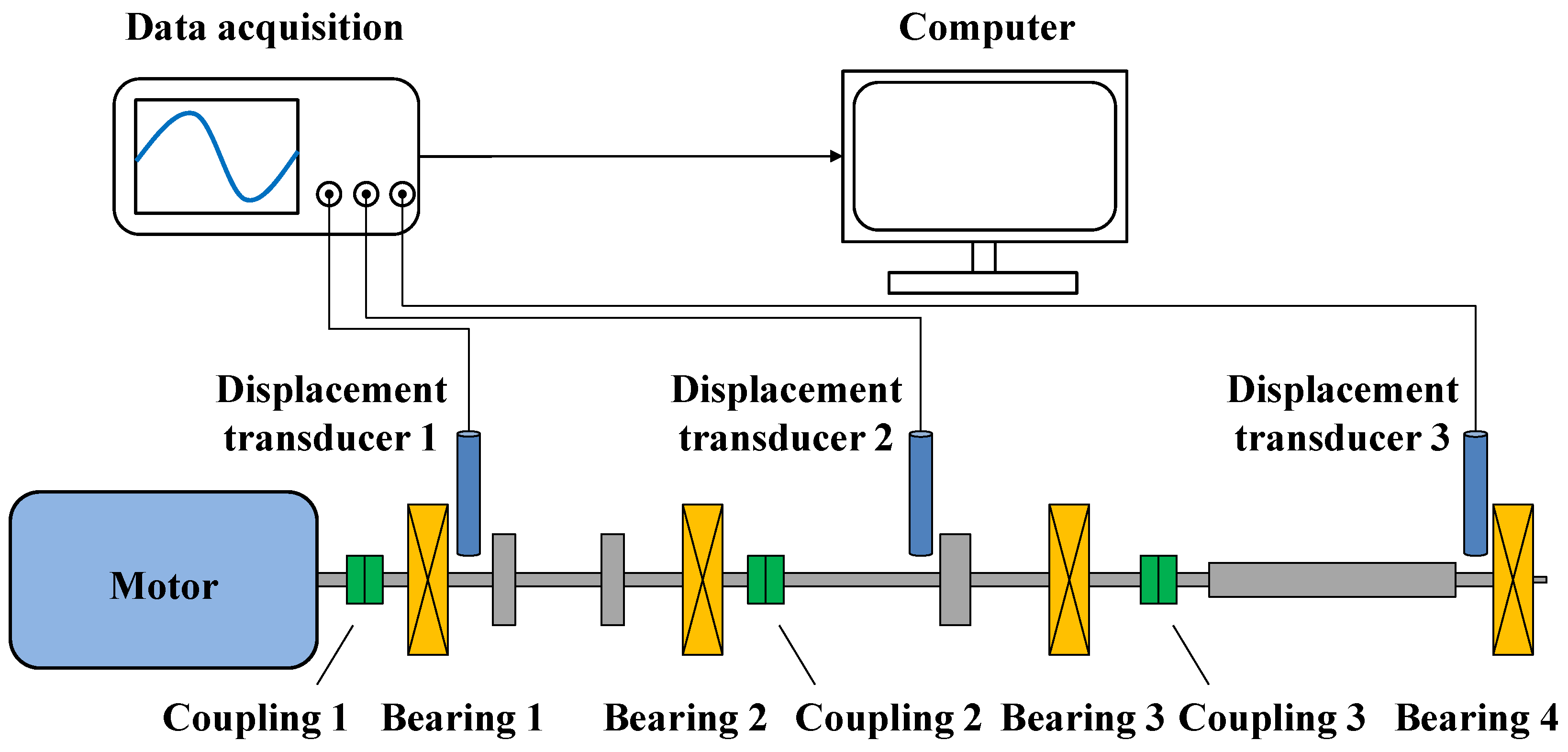
2.1. Signals Collection

The experimental platform for crack fault detection of asymmetric shafting is designed and built based on a ZT-3 platform. The schematic diagram of the experimental platform is shown in Figure 1, and the physical diagram is shown in Figure 2. The platform is composed of an asymmetric shaft body, a drive system and a measurement system. The asymmetric shaft body consists of three rotors. Taking the DC motor end as left, from left to right, respectively, there is a double disk rotor, a single disk rotor and a generator rotor. Bearings 1, 2 and 3 are rolling bearings, and bearing 4 is a sliding bearing. The length of the three rotors is 320 mm. The diameters of the double-disk rotor shaft, the single-disk rotor shaft and the generator rotor shaft are 9.5 mm. The diameter and thickness of the double disk rotor disc are 76 mm and 19 mm, respectively, and the diameter and thickness of the single disk rotor disc are 76 mm and 25 mm, respectively.

The drive system consists of a speed governor and a DC motor. The DC motor drives an asymmetric shaft system through a coupling. The measuring system consists of a DC regulated power supply, an eddy current displacement sensor and a data acquisition instrument, as shown in Figure 3. The DC regulated power supply provides voltage to the eddy current displacement sensor. When the distance between the rotor and the sensor changes, the dynamic voltage signal generated by the sensor is transmitted to the data collector. The platform contains three eddy current displacement sensors, which are, respectively, used to pick up the vibration displacement signals of the double-disk rotor, the single-disk rotor and the generator rotor near the bearing. The rotors is shown in Figure 4a–c. In order to avoid interference between eddy current displacement sensors, sensors are arranged only in the horizontal direction. Subsequent research shows that the use of only a horizontal displacement signal can also ensure high fault detection accuracy. The data collector uses a DASH8HF-HS system; the sampling rate is set to 20 kHz.

In order to simulate the crack fault, a crack with a depth of 2.4 mm was machined on the shafts of the double-disk rotor and the single-disk rotor by wire cutting. The ratio of the crack depth to the shaft diameter was about 0.25. The diagrams of a healthy rotor and a cracked rotor are shown in Figure 5. This paper studies cracks in four different locations. The cracks are machined at a location away from the center of the shaft in order to simulate two different locations of the crack by turning the crack shaft upside down left and right during the experiment. According to the above description, the distances between the cracks at four different locations and the left end of the asymmetric shaft system are 100 mm (Case 1), 220 mm (Case 2), 420 mm (Case 3) and 540 mm (Case 4), respectively. The cracks in Case 1 and Case 2 are located on the double disk rotor, while the cracks in Case 3 and Case 4 are located on the single disk rotor. Case 1 and case 2 and Case 3 and Case 4 are centrosymmetric about the double disk rotor and the single disk rotor, respectively. The shaft without cracks is called a healthy rotor, denoted as Case 0.

This section collects the vibration signals at three channels when the rotating speed is 2000 rpm, that is, the vibration signals of the double disk rotor, the single disk rotor and the generator rotor along the horizontal direction. There are five working conditions for no crack (Case 0), the double disk rotor left crack (Case 1), the double disk rotor right crack (Case 2), the single disk rotor left crack (Case 3) and the single disk rotor right crack (Case 4). The sampling frequency is 20 kHz, and each acquisition is 10 s, that is, 200,000 sampling points for each working condition. At the above speeds and sampling frequencies, there are 600 sampling points per cycle. In order to ensure that each sample contains at least 3 cycles, the data length of each sample point is set to 2048. In order to ensure the training accuracy of the fault detection model, the total sample size is 1000, and the data is enhanced by overlapping sampling techniques, as shown in Figure 6. If we move the window of the first signal along the timing direction, the slip is less than the length of the signal segment, and there will be a certain overlap between the first segment and the second segment. In this way, more samples can be generated from a long signal, which achieves data enhancement.

In this paper, the convolution neural network is adopted to extract the fault feature of the experimental signal to complete the classification task of crack location. To extract the fault feature, the convolution layer and the fully connected layer are needed. In order to measure the error of fault detection, it is necessary to define the loss function, also known as the objective function. In the training process of the network, an optimization algorithm is needed to update the hyperparameters of the network so that the hyperparameters in the network can be updated stably in the direction of minimizing the loss function to ensure the fault detection accuracy of the model. The loss function and optimization algorithm of a convolutional neural network are introduced below.

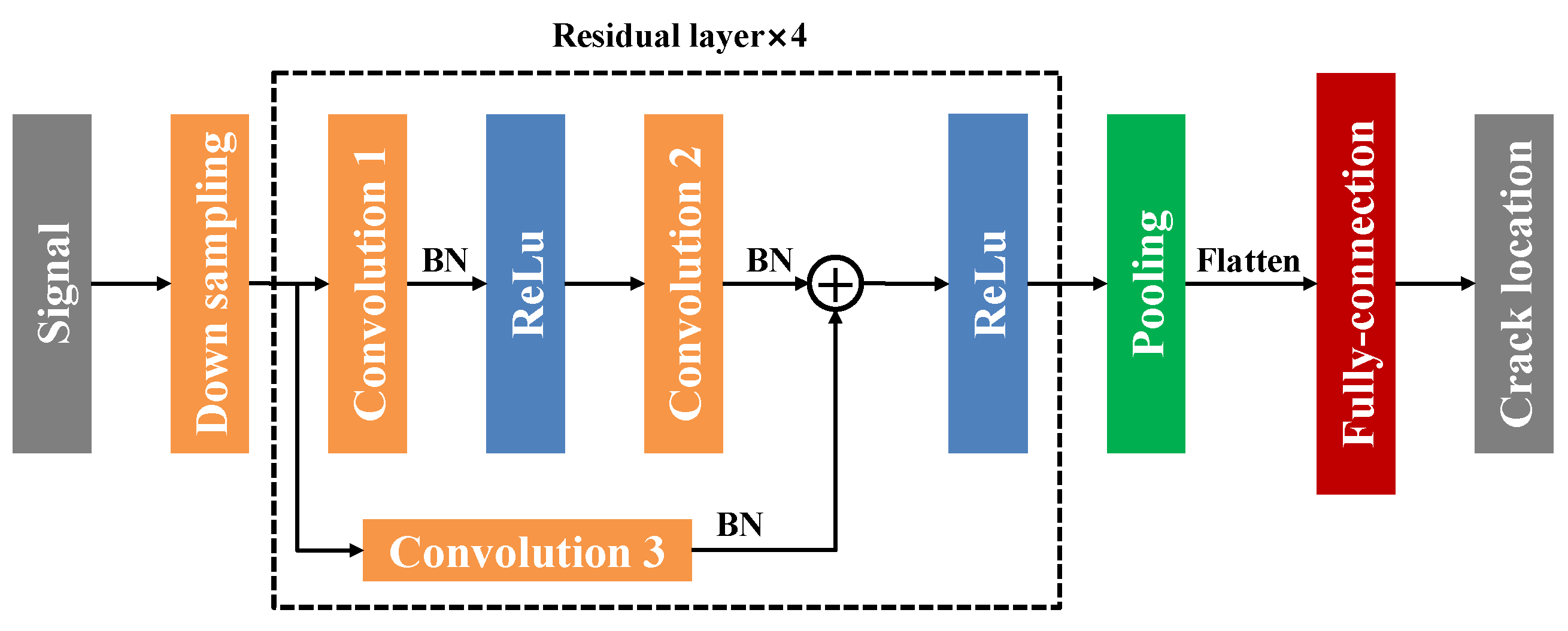
2.2. Convolutional Layer

A convolution operation refers to the use of multiple convolution kernels to multiply the coefficients of the corresponding location in the local area of the input signal to achieve feature extraction. The main advantages of a convolution operation are weight sharing and sparse connection, which can reduce the number of hyperparameters to be trained and the amount of calculation. A convolutional layer operation is defined as:

$${\mathit{x}}_i^{(l)}=\phi \left({\left({\mathit{k}}^{(l)}\right)}^T{\mathit{x}}_i^{(l-1)}+b_c^{(l)}\right)$$

(1)

where $\phi$ denotes convolution operation, ${\mathit{k}}^{(l)}$ is the kernel weight of the lth convolution layer, $b_c^{(l)}$ is the bias of the lth convolution layer, ${\mathit{x}}_i^{(l)}$ is the output of the lth, i denotes the sample number, and ${\mathit{x}}_i^{(l-1)}$ is the input of the lth.

Usually, a batch normalization layer (BN) needs to be connected after the convolution layer. The batch normalization layer is designed to alleviate the ‘gradient dispersion’ problem in deep networks and accelerate model convergence. The operation of a batch normalization layer can be expressed as:

$${\widehat{\mathit{x}}}_i^{(l)}=\frac{{\mathit{x}}_i^{(l)}-E\left[{\mathit{x}}_i^{(l)}\right]}{\sqrt{Var\left[{\mathit{x}}_i^{(l)}\right]}}$$

(2)

$${\mathit{x}}_i^{(l)}=\kappa {\widehat{\mathit{x}}}_i^{(l)}+\tau$$

(3)

where $E$ is the expectation, $Var$ is the variance, $\kappa$ is the scale factor, and $\tau$ is the translation factor.

After the batch normalization layer, an activation function needs to be connected to improve the nonlinear expression ability of the neural network. A rectified linear unit is adopted in this paper:

$${\mathit{r}}_i^{(l)}=\max (0,{\mathit{x}}_i^{(l)})$$

(4)

In addition, layer skip layer connection is designed to overcome the problems of gradient dispersion and gradient explosion of a neural network and accelerate convergence [34].

2.3. Fully Connected Layer

The full connection layer acts as a classifier in the entire neural network. In the conventional method, before inputting the features learned from the convolution layer into the full connection layer, the features need to be regularized and flattened. In this paper, the average pooling layer is added before the full connection layer to reduce the feature dimensions and then flattened. The average pooling operation is defined as:

$${({\mathit{v}}_i^{(le+1)})}_{k,m}=[\frac{1}{j}{\displaystyle \sum _{g=1}^j{r}_{i,g,m}^{le}}|j\in N^{+},s(k-1)+1\le j\le sk,\forall r_{i,j,m}^{le}\in {\mathit{r}}_i^{le}]$$

(5)

where ${\mathit{v}}_i^{(le+1)}$ is the characteristics after pooling.

After flattening the extracted features and inputting them into the full connection layer, it can be obtained that:

$${\mathit{h}}_{i,j}=\sigma ({\mathit{w}}^T{\mathit{o}}_i+b_f)$$

(6)

where $\mathit{w}$ is the weight, $b_f$ is the bias, and ${\mathit{h}}_{i,j}$ is the output of the fully connected layer.

Output can be converted into probability distribution of sample labels by the SoftMax function:

$$P(y_i=j|{\mathit{h}}_{i,j})=\frac{\exp ({\mathit{h}}_{i,j})}{{\displaystyle \sum _{j=1}^C\exp ({\mathit{h}}_{i,j})}}$$

(7)

where $y_i$ is the real label of the ith sample, and $C$ is the classification number:

2.4. Loss Function

In the classification task, cross entropy measures the distance between the real distribution and the above probability distribution, which can be regarded as a loss function to optimize the neural network. The loss function in this paper is:

$$L=\frac{1}{B}{\displaystyle \sum _{i=1}^B{\displaystyle \sum _{j=1}^C-y_i\log \left(P(y_i=j|{\mathit{h}}_{i,j})\right)}}$$

(8)

where L denotes loss function, and B is the batch number.

2.5. Optimization Algorithm

The Adam optimizer is usually used to train network parameters [35]. It combines the advantages of AdaGrad and RMSProp and has the advantages of easy parameter adjustment and fast convergence. The process from Equations (1)–(8) can be expressed as:

$$L=J(\mathit{x},\mathit{y},\mathit{\theta })$$

(9)

where x is the input signal, and θ is all trainable hyperparameters of fault detection model. The update rules for trainable parameters are as follows:

$$g={\nabla }_{\theta }J(\mathit{\theta })$$

(10)

$$m={\beta }_{1}m+(1-{\beta }_1)g$$

(11)

$$t={\beta }_{2}t+(1-{\beta }_2)g^2$$

(12)

$$\widehat{m}=m/(1-{\beta }_1)$$

(13)

$$\widehat{t}=t/(1-{\beta }_2)$$

(14)

$$\mathit{\theta }=\mathit{\theta }-\alpha \ast \widehat{m}/\left(\sqrt{\widehat{t}}+\epsilon \right)$$

(15)

where ${\beta }_1$, ${\beta }_2$ are the exponential decay rate, $\epsilon$ is an almost zero decimal, and α is the learning rate. The learning rate is calculated as follows [36]:

$${\alpha }_i={\alpha }_0/{\left(1+10e_i/epoch\right)}^{0.75}$$

(16)

where epoch is the total iteration steps, and $e_i$ is the current iteration steps.

The proposed fault detection network is shown in Figure 7, and the corresponding model parameters are shown in

Table 1. Parameters of the fault detection model.

Numbering	Layers	Kernel Size	Stride	Channels	Output Size (Width × Depth)
1	Down-sampling	64 × 1	8 × 1	32	256 × 32
2	Residual layer 1	$\{\begin{array}{c}CK1=3\times 1\\ CK2=3\times 1\\ CK3=1\times 1\end{array}$	$\{\begin{array}{c}CS1=2\times 1\\ CS2=1\times 1\\ CS3=2\times 1\end{array}$	32	128 × 32
3	Residual layer 2			64	64 × 64
4	Residual layer 3			128	32 × 128
5	Residual layer 4			256	16 × 256
6	Pooling	4 × 1	4 × 1	256	4 × 256
7	Flatten	-	-	-	1024
8	Fully connected	1024	-	1	1024 × 1
9	Softmax	5	-	1	5

. Where, CK1 to CK3 represent the kernel sizes of convolution in the residual layer in Figure 7, and CK1 to CK3 represent Stride, respectively. The model contains four residual layers. The length of the time-domain signal for a single sample is 2048, and the channel is 3. The vibration displacement signal is collected by three sensors. Firstly, the original signal is input into a down-sampling layer (i.e., a convolution layer) and becomes data with a width of 256 and a depth of 32. Then, after 4 residual layers, it becomes data with a width of 4 and a depth of 256. Finally, through a pooling operation, a flatten operation and a fully connected layer, the classification probability is output to further complete the detection of crack location. Before training the fault detection model, the total sample is divided into a training and a test set, as shown in Figure 6. Without special instructions, we use the first 70% of the total sample as the training set and the remaining 20% as the test set, and we remove the middle 10%. In the training process, no noise is added to the training set; only Gaussian noise is added to the test set.

3. The Evaluation Indicators

For the fault diagnosis task, the classification accuracy is used as the evaluation index, and the confusion matrix is also used to evaluate the classification accuracy, Wen et al. [22]. For the true value y and the predicted value $\widehat{y}$, the formula for calculating the classification accuracy is:

$$A(y,\widehat{y})=[{\displaystyle \sum _{(\mathbf{X},y)\in {\mathbf{\Omega }}_{\mathrm{test}}}{\rm I}(y=\widehat{y})}]/N{\mathbf{\Omega }}_{\mathrm{test}}$$

(17)

where ${\mathbf{\Omega }}_{\mathrm{test}}$ is the test set sample space.

4. Results and Discussion

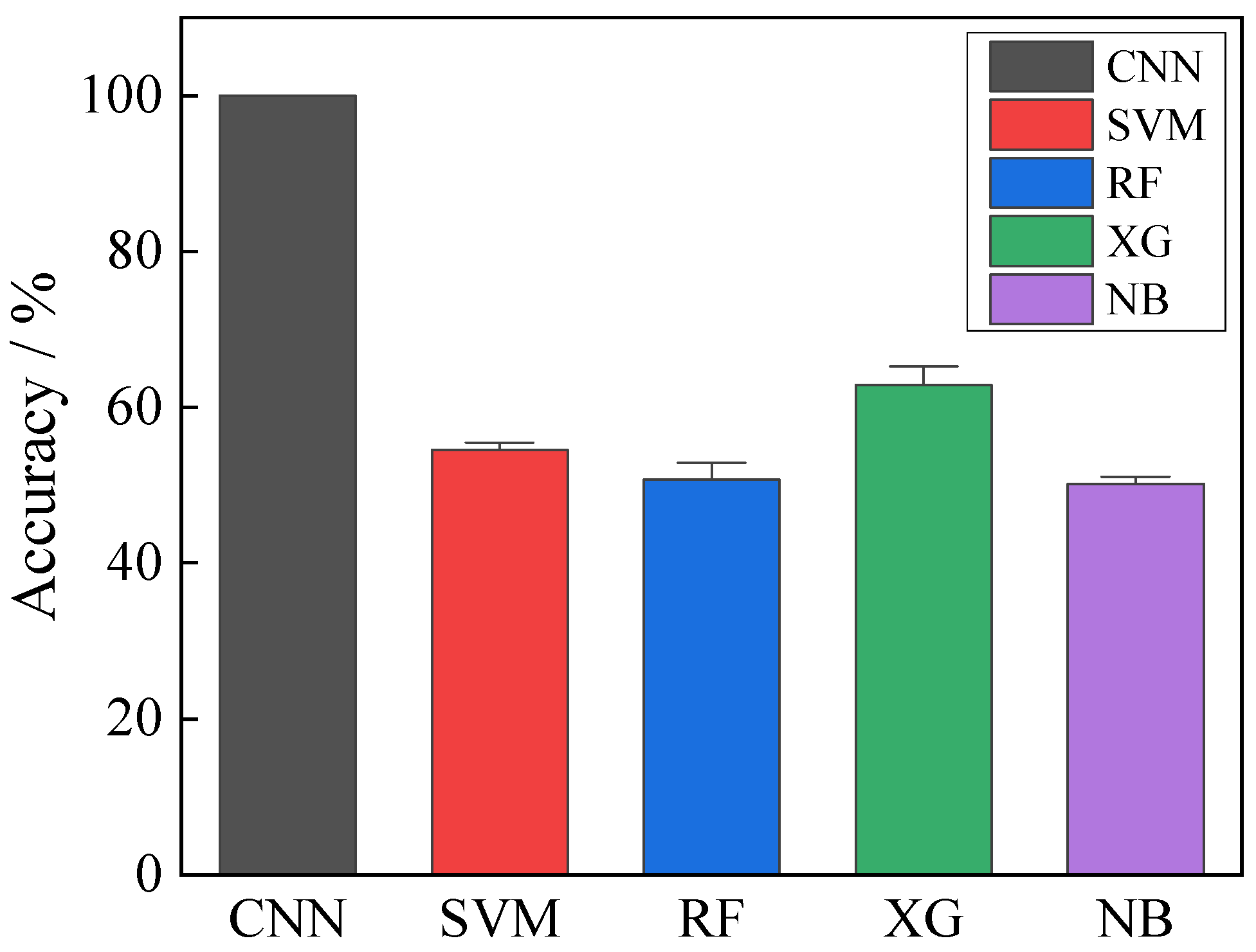
4.1. Evaluation of the Proposed Method

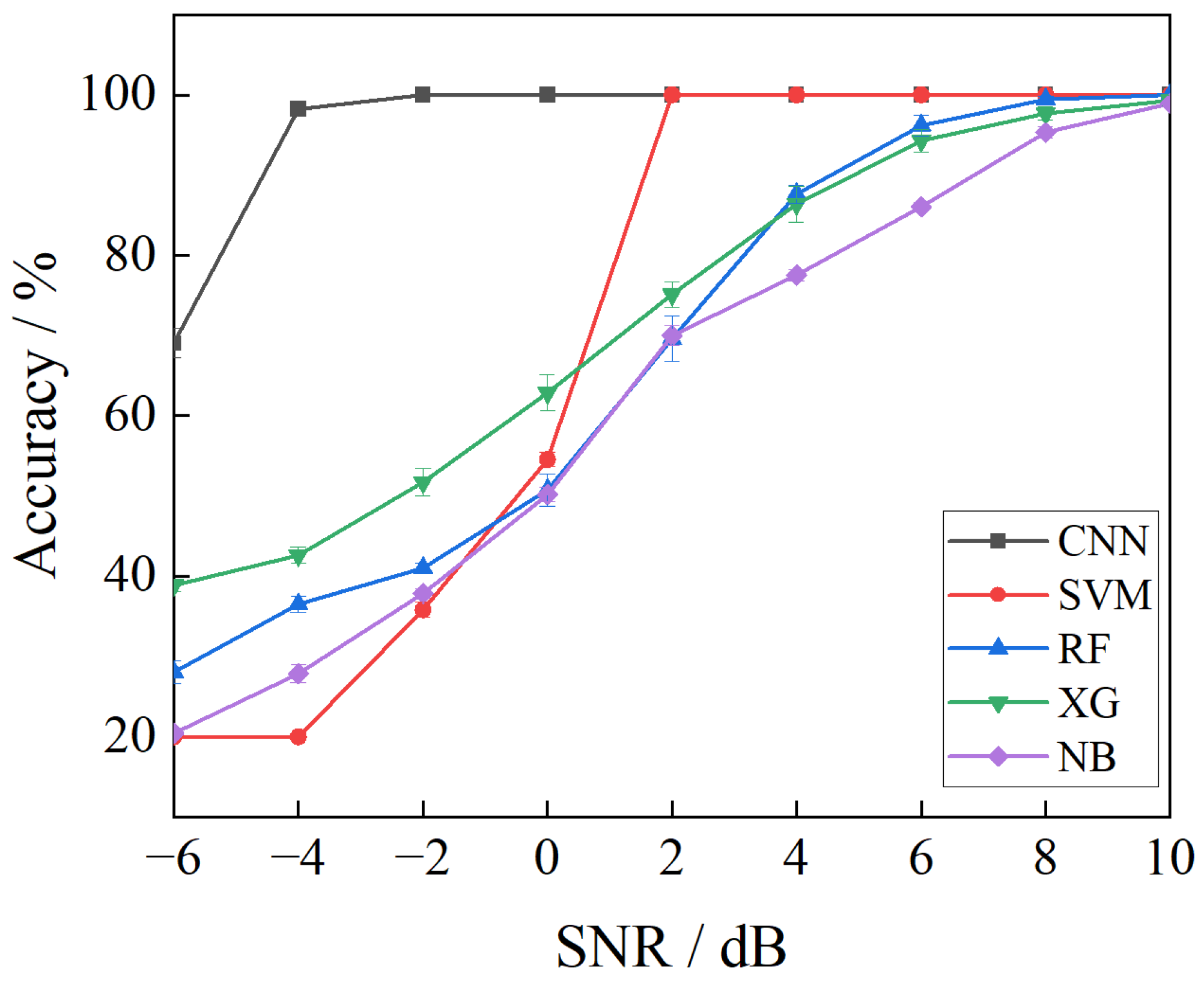
Figure 8 shows the results of the accuracy and standard deviation between the crack location detection in this paper and the other four common machine algorithms in crack location detection. The above data are obtained by 10 tests on the same model. The signal-to-noise ratio is 0, that is, the noise and signal power are equal. CNN represents the convolutional neural network-based method proposed in this paper. SVM, RF, XG and NB represent support vector machine, random forest, Xgboost and naive Bayesian algorithms, respectively. It can be seen from the figure that the average accuracy of the model, support vector machine, random forest, Xgboost and naive Bayesian algorithm in crack location detection are 100%, 54.5%, 49.5%, 62.5% and 51.5%, respectively. The accuracy of this model is the highest. In addition, it can be found that in the 10 tests, the accuracy of the proposed method is 100%, and the standard deviation is almost 0. However, the accuracy of the other machine learning algorithms are not the same in the 10 tests, and there is a certain standard deviation.

Figure 9 shows the confusion matrix of the crack location detection in this paper, whose horizontal coordinates represent the detection label, and the ordinates represent the real label. The value in the matrix represents the proportion of the number of samples detected as a row label by a signal actually belonging to a column label. The closer the value on the diagonal is to one, the better the effect of the detection model is. It can be seen from the figure that when the signal-to-noise ratio is equal to zero0, the diagonals of the confusion matrix are all one, indicating that the fault detection model can accurately classify healthy rotors and crack faults at four different locations.

Figure 10 shows the visualization process of the model in crack location detection. The results shown in the figure are the distribution of the output of each residual layer in two-dimensional space after t-SNE dimensionality reduction. As can be seen from the figure, with the increase in the number of residual layers, the distinguishability of the five fault signals becomes stronger and stronger, and the indistinguishable signals in the low-dimensional space gradually become distinguishable in the high-dimensional space. This shows that it is important to increase the depth of the convolution network. After the first residual layer and the second residual layer, the characteristic distribution of the five working conditions is not obvious. The characteristics of the same working condition gather in different regions on the two-dimensional plane, and the aggregation degree is not close. This shows that the separability and robustness of each working condition are impotent. After the third residual layer, there is no cross between the characteristics of the healthy rotor condition (Case 0) and the two crack conditions on the single disk rotor (Case 3 and Case 4). The characteristics of the training set and the test set are basically clustered in the same area, which shows that the fault detection model has strong ability to distinguish the above three faults. However, it can be observed that in Case 1 and Case 2, the sample characteristics of the two conditions overlap, which shows that the model has difficulty distinguishing the above two conditions. After the fourth residual layer, the sample characteristics of the five fault conditions are clustered in the same area and far from each other. This shows that the classification accuracy of the model is high. In addition, the sample characteristics of the training and test sets overlap almost entirely under various operating conditions, indicating that the generalization ability of the model is strong.

4.2. Impact of SNR

This section studies the influence of the signal-to-noise ratio on the performance of the crack location detection network. In this section, the performance of five algorithms for crack location detection at an SNR of −6 dB to 10 dB is analyzed. The corresponding results are shown in Figure 11. The number of training samples is 700. It can be seen from the figure that when the SNR is 10 dB, that is, when the ratio of signal power to noise power is large, the average accuracy of the five algorithms is above 98%, and the accuracy is almost unchanged. Among them, the average accuracy of the model proposed in this paper, support vector machine and random forest reach 100%, with high accuracy. When the signal-to-noise ratio decreases from 10 dB to 2 dB, the accuracy of random forest, Xgboost and naive Bayesian algorithms will decrease significantly with the increase of noise power. However, the average accuracy of the model proposed in this paper and the support vector machines, which are always 100%, do not decrease, and the detection effect is good. When the signal-to-noise ratio decreases from 2 dB to-6 dB, the five algorithms decrease significantly with the increase of noise power. When the signal-to-noise ratio is −2 dB and −4 dB, that is, the noise power exceeds the signal power, the average accuracy of the model proposed in this paper is the highest, which is 100% and 98.2%, respectively, while the accuracy of the other four machine learning algorithms is less than 52%, and the detection effect is poor. When the SNR is −6 dB, the average accuracy of the model proposed in this chapter is 69%, and the classification effect is poor. However, the accuracy of the other four machine learning algorithms are lower than 40%, which is lower than the model proposed in this paper. From the above analysis, the model has the highest accuracy under the signal-to-noise ratio of-6 dB to 10 dB, and the anti-noise performance is stronger than the traditional machine learning algorithm.

Figure 12 shows the confusion matrix of the crack location detection model established in this paper when the SNR is −6 dB to −4 dB. It can be seen from Figure 12a that when the signal-to-noise ratio is −6 dB, 41% and 57% of the samples in the healthy rotor (Case 0) are detected as cracks on the left side of the double-disk rotor (Case 1) and cracks on the right side of the double-disk rotor (Case 2), respectively. This shows that when the noise power is high, the healthy rotor is easier to be confused with cracks on the double-disk rotor, resulting in wrong classification results. Among the samples of double disk rotor left crack (Case 1), 13% and 21% of the samples were misclassified as double disk rotor right crack (Case 2) and single disk rotor left crack (Case 3), respectively. Among the samples of the right side crack (Case 2) of the double disk rotor, 38% of the samples were misclassified as the left side crack (Case 3) of the single disk rotor, indicating that the cracks on the double-disk rotor are more easily confused with the cracks on the single-disk rotor. The accuracy of the single disk rotor crack (Case 3 and Case 4) is 97% and 100%, respectively, while only 3% of the sample of Case 3 is misclassified as Case 2. From the above analysis, it can be seen that under the influence of noise, the real signal is easily misclassified as working conditions close to it in the physical location. Figure 12b shows that when the signal-to-noise ratio is −4, only 3% of the healthy rotor (Case 0) are misclassified as the right side crack of double disk rotor (Case 2), while the accuracy of the other cases is 100%. Under the above two signal-to-noise ratios, the accuracy of the healthy rotor is the lowest. This shows that the increase of the noise power makes the signal of the healthy rotor easy to be misclassified as other working conditions.

4.3. Effect of the Number of Training Samples

This section studies the effect of the number of training samples on the performance of the crack location detection network. In this section, the performance of the crack location detection model based on the convolutional neural network algorithm is analyzed in the case of 100, 300, 500 and 700 training samples, respectively. The corresponding results are shown in Figure 13. The figure shows that when the signal-to-noise ratio is equal to 10 dB, that is, the signal power is much larger than the noise power, the accuracy of the 4 training samples is 100%, and the accuracy is high. The more training samples there are, the higher the accuracy of the fault detection network is. With the increase of noise power, that is, with the decrease of the signal-to-noise ratio, the accuracy will decrease obviously when the number of training samples is 100. The average accuracy can maintain a high value in a wide range of the signal-to-noise ratio when the number of training samples is 700. Even when the signal-to-noise ratio is −4 dB, the accuracy is still greater than 98%, indicating that when the number of samples is high, the fault detection network has low requirements for the cleanliness of the signal, which is suitable for the application in the actual industrial scene. The above analysis shows that the number of training samples plays a decisive role in the recognition rate and anti-noise ability of the fault detection network. It also shows that when the sample size is not enough, the strategy of overlapping sampling for data enhancement is effective.

Figure 14 shows the confusion matrix of the crack location detection model established in this paper when the number of training samples is 300 and 500, and the value of the signal-to-noise ratio is 0 dB. It can be seen from Figure 14a that when the number of training samples is 300, the accuracy of the healthy rotor (Case 0), the double-disk rotor right crack (Case 2) and the single-disk rotor right crack (Case 4) are higher, which are 100%, 100% and 99%, respectively.

In addition, only 1% of the samples in Case 4 are misclassified as Case 0. In the samples of the left crack of the double-disk rotor (Case 1), 33% and 19% of the samples are detected as Case 0 and Case 2. In the samples of the left crack of the single-disk rotor (Case 3), 49% and 5% of the samples are detected as Case 0 and Case 2. In Case 1 and Case 3, samples are easily misclassified as healthy rotors. Figure 14b shows that when the number of training samples is 500, only 7% of the samples which are the left crack (Case 1) of the double disc rotor are misclassified as the right crack (Case 2) of the double disc rotor, while the accuracy of other cases is 100%. The accuracy of Case 1 and Case 3 is the lowest under the above two training samples. This shows that the reduction of the number of training samples makes the above crack conditions easily misclassified as other conditions.

5. Conclusions and Future Works

In this paper, an experimental platform for the detection of crack faults in asymmetric shaft systems is designed and built independently. The experimental vibration data are collected, and the end-to-end crack location detection model based on a convolutional neural network is proposed. The influencing factors and effects of fault detection accuracy are deeply studied. The main conclusions are as follows: By comparing the accuracy of the method, support vector machine, random forest, xgboost and naive Bayesian algorithm in crack location detection task, it can be found that when the signal-to-noise ratio is 0 dB, the average accuracy of the method proposed is 100%, while the maximum accuracy of other machine learning algorithms is no more than 63%; thus the accuracy of this model is the highest. By comparing the method in this paper and the other four machine learning algorithms under different signal-to-noise ratios, it can be found that the method in this paper has the highest accuracy and the strongest anti-noise ability under the signal-to-noise ratio of −6 dB to 10 dB. By comparing the model in this paper with different training sample numbers, the number of training samples plays a decisive role in the accuracy and anti-noise ability of the fault detection network. The strategy of data enhancement by overlapping sampling is effective. In addition, by analyzing the confusion matrix under a different number of training samples, it can be found that the reduction of the number of training samples makes the cracks on the right side of the single disk rotor and the double disk rotor easy to be misclassified into other working conditions.

This research has great applicability prospects for carrying out a fault detection method based on the combination of deep learning and experiment and migrating it to practical industrial applications. This paper only considers the study pd crack faults of asymmetric shafting. In the future, we will carry out more experimental research on rotor fault types, enrich the data set and further carry out the study on the transfer and application of this model to actual industrial data.

References

1. Bachschmid, N.; Pennacchi, P.; Vania, A. Identification of multiple faults in rotor systems. J. Sound Vib. 2002, 254, 327–366. [Google Scholar] [CrossRef] [Green Version]
2. Friswell, M.I.; Penny, J.E.T.; Garvey, S.D.; Lees, A.W. Dynamics of Rotating Machines; Cambridge University Press: Cambridge, UK, 2010. [Google Scholar]
3. Sekhar, A. Crack identification in a rotor system: A model-based approach. J. Sound Vib. 2003, 270, 887–902. [Google Scholar] [CrossRef]
4. Sekhar, A. Model-based identification of two cracks in a rotor system. Mech. Syst. Signal Process. 2004, 18, 977–983. [Google Scholar] [CrossRef]
5. Chen, X.F.; Bing, L.; Qiao, H. Crack Fault Diagnosis Based on Wavelet Finite Elements. J. Xi’an Jiaotong Univ. 2004, 38, 295–298. [Google Scholar]
6. Babu, T.R.; Sekhar, A. Detection of two cracks in a rotor-bearing system using amplitude deviation curve. J. Sound Vib. 2008, 314, 457–464. [Google Scholar] [CrossRef]
7. Varney, P.; Green, I. Rotordynamic Crack Diagnosis: Distinguishing Crack Depth and Location. J. Eng. Gas Turbines Power 2013, 135, 112101. [Google Scholar] [CrossRef]
8. Haji, Z.N.; Oyadiji, S.O. The use of roving discs and orthogonal natural frequencies for crack identification and location in rotors. J. Sound Vib. 2014, 333, 6237–6257. [Google Scholar] [CrossRef]
9. Söffker, D.; Wei, C.; Wolff, S.; Saadawia, M.-S. Detection of rotor cracks: Comparison of an old model-based approach with a new signal-based approach. Nonlinear Dyn. 2015, 83, 1153–1170. [Google Scholar] [CrossRef]
10. Gupta, R.B.; Singh, S.K. Detection of crack and unbalancing in a rotor system using artificial neural network. In Proceedings of the First International Conference on Future Learning Aspects for Mechanical Engineering, Noida, India, 3–5 October 2018; pp. 607–618. [Google Scholar]
11. Sathujoda, P. Detection of a slant crack in a rotor bearing system during shut-down. Mech. Based Des. Struct. Mach. 2020, 48, 266–276. [Google Scholar] [CrossRef]
12. Bachschmid, N.; Pennacchi, P.; Tanzi, E.; Vania, A. Identification of transverse crack location and depth in rotor systems. Meccanica 2000, 35, 563–582. [Google Scholar] [CrossRef] [Green Version]
13. Pennacchi, P.; Bachschmid, N.; Vania, A. A model-based identification method of transverse cracks in rotating shafts suitable for industrial machines. Mech. Syst. Signal Process. 2006, 20, 2112–2147. [Google Scholar] [CrossRef]
14. Yao, H.; Li, H. Diagnoses of coupling fault of crack and rub-impact in rotor systems. J. Vib. Eng. 2006, 19, 307–312. [Google Scholar]
15. Dong, H.; Chen, X.; Li, B.; Qi, K.; He, Z. Rotor crack detection based on high-precision modal parameter identification method and wavelet finite element model. Mech. Syst. Signal Process. 2009, 23, 869–883. [Google Scholar] [CrossRef]
16. Janssens, O.; Slavkovikj, V.; Vervisch, B.; Stockman, K.; Loccufier, M.; Verstockt, S.; Van de Walle, R.; Van Hoecke, S. Convolutional Neural Network Based Fault Detection for Rotating Machinery. J. Sound Vib. 2016, 377, 331–345. [Google Scholar] [CrossRef]
17. Zhang, W.; Peng, G.; Li, C.; Chen, Y.; Zhang, Z. A New Deep Learning Model for Fault Diagnosis with Good Anti-Noise and Domain Adaptation Ability on Raw Vibration Signals. Sensors 2017, 17, 425. [Google Scholar] [CrossRef] [PubMed] [Green Version]
18. Zhang, W.; Li, C.; Peng, G.; Chen, Y.; Zhang, Z. A deep convolutional neural network with new training methods for bearing fault diagnosis under noisy environment and different working load. Mech. Syst. Signal Process. 2018, 100, 439–453. [Google Scholar] [CrossRef]
19. Yuan, Z.; Zhang, L.; Duan, L. A novel fusion diagnosis method for rotor system fault based on deep learning and multi-sourced heterogeneous monitoring data. Meas. Sci. Technol. 2018, 29, 115005. [Google Scholar] [CrossRef]
20. Han, T.; Liu, C.; Yang, W.; Jiang, D. Deep transfer network with joint distribution adaptation: A new intelligent fault diagnosis framework for industry application. ISA Trans. 2020, 97, 269–281. [Google Scholar] [CrossRef] [Green Version]
21. Yang, B.; Lei, Y.; Jia, F.; Xing, S. An intelligent fault diagnosis approach based on transfer learning from laboratory bearings to locomotive bearings. Mech. Syst. Signal Process. 2019, 122, 692–706. [Google Scholar] [CrossRef]
22. Wen, L.; Gao, L.; Li, X. A New Deep Transfer Learning Based on Sparse Auto-Encoder for Fault Diagnosis. IEEE Trans. Syst. Man Cybern. Syst. 2019, 49, 136–144. [Google Scholar] [CrossRef]
23. Wang, C.; Zhu, G.; Liu, T.; Xie, Y.; Zhang, D. A sub-domain adaptive transfer learning base on residual network for bearing fault diagnosis. J. Vib. Control. 2021, 29, 105–117. [Google Scholar] [CrossRef]
24. Ren, Z.; Zhu, Y.; Yan, K.; Chen, K.; Kang, W.; Yue, Y.; Gao, D. A novel model with the ability of few-shot learning and quick updating for intelligent fault diagnosis. Mech. Syst. Signal Process. 2020, 138, 106608. [Google Scholar] [CrossRef]
25. Zhang, A.; Li, S.; Cui, Y.; Yang, W.; Dong, R.; Hu, J. Limited Data Rolling Bearing Fault Diagnosis With Few-Shot Learning. IEEE Access 2019, 7, 110895–110904. [Google Scholar] [CrossRef]
26. Zhu, X.; Hou, D.; Zhou, P.; Han, Z.; Yuan, Y.; Zhou, W.; Yin, Q. Rotor fault diagnosis using a convolutional neural network with symmetrized dot pattern images. Measurement 2019, 138, 526–535. [Google Scholar] [CrossRef]
27. Gao, Y.; Liu, X.; Huang, H.; Xiang, J. A hybrid of FEM simulations and generative adversarial networks to classify faults in rotor-bearing systems. ISA Trans. 2020, 108, 356–366. [Google Scholar] [CrossRef]
28. Lei, Y.; Yang, B.; Jiang, X.; Jia, F.; Li, N.; Nandi, A.K. Applications of machine learning to machine fault diagnosis: A review and roadmap. Mech. Syst. Signal Process. 2020, 138, 106587. [Google Scholar] [CrossRef]
29. Nath, A.G.; Udmale, S.S.; Singh, S.K. Role of artificial intelligence in rotor fault diagnosis: A comprehensive review. Artif. Intell. Rev. 2020, 54, 2609–2668. [Google Scholar] [CrossRef]
30. Dou, Z.; Sun, Y.; Wu, Z.; Wang, T.; Fan, S.; Zhang, Y. The Architecture of Mass Customization-Social Internet of Things System: Current Research Profile. ISPRS Int. J. Geo-Inf. 2021, 10, 653. [Google Scholar] [CrossRef]
31. Zhu, J.; Gong, Z.; Sun, Y.; Dou, Z. Chaotic neural network model for SMISs reliability prediction based on interdependent network SMISs reliability prediction by chaotic neural network. Qual. Reliab. Eng. Int. 2020, 37, 717–742. [Google Scholar] [CrossRef]
32. Liu, K.; Yu, Q.; Liu, Y.; Yang, J.; Yao, Y. Convolutional Graph Thermography for Subsurface Defect Detection in Polymer Composites. IEEE Trans. Instrum. Meas. 2022, 71, 1. [Google Scholar] [CrossRef]
33. Liu, K.; Zheng, M.; Liu, Y.; Yang, J.; Yao, Y. Deep Autoencoder Thermography for Defect Detection of Carbon Fiber Composites. IEEE Trans. Ind. Informatics 2022. [CrossRef]
34. He, K.; Zhang, X.; Ren, S.; Sun, J. Deep Residual Learning for Image Recognition. In Proceedings of the IEEE Conference on Computer Vision and Pattern Recognition, Las Vegas, NV, USA, 27–30 June 2016; pp. 770–778. [Google Scholar]
35. Kingma, D.; Ba, J. Adam: A method for stochastic optimization. In Proceedings of the International Conference on Learning Representations, San Juan, Puerto Rico, 2–4 May 2016. [Google Scholar]
36. Ganin, Y.; Ustinova, E.; Ajakan, H.; Germain, P.; Larochelle, H.; Laviolette, F.; Marchand, M.; Lempitsky, V. Domain-Adversarial Training of Neural Networks. J. Mach. Learn. Res. 2016, 17, 1–35. [Google Scholar] [CrossRef]
Figure 1. Schematic diagram of the experimental platform for crack fault detection in asymmetric shafts.
Applsci 13 01327 g001
Figure 2. Experimental platform for crack fault detection in asymmetric shafts.
Applsci 13 01327 g002
Figure 3. Measuring system.
Applsci 13 01327 g003
Figure 4. Diagram of asymmetric shaft system; (a) dual-disk rotor; (b) single disk rotor; (c) generator rotor.
Applsci 13 01327 g004
Figure 5. Physical diagram of a healthy rotor and a cracked rotor: (a) healthy rotor; (b) cracked rotor.
Applsci 13 01327 g005
Figure 6. Overlap sampling.
Applsci 13 01327 g006
Figure 7. Fault detection model based on a convolutional neural network.
Applsci 13 01327 g007
Figure 8. Comparison of different algorithms in crack location detection.
Applsci 13 01327 g008
Figure 9. Confusion matrix of this model.
Applsci 13 01327 g009
Figure 10. Visualization of crack location detection process: (a) residual layer 1; (b) residual layer 2; (c) residual layer 3; (d) residual layer 4.
Applsci 13 01327 g010
Figure 11. Influence of SNR on accuracy.
Applsci 13 01327 g011
Figure 12. Confusion matrix under different SNR: (a) SNR = −6; (b) SNR = −4.
Applsci 13 01327 g012
Figure 13. Influence of training set sample number on accuracy.
Applsci 13 01327 g013
Figure 14. Confusion matrix under different numbers of training samples: (a) training samples = 300; (b) training samples = 500.
Applsci 13 01327 g014