Analysis of Bifurcation Vibrations of an Industrial Robot Arm System with Joints Compliance

Abstract

This paper deals with the analysis of nonlinear vibration phenomena in the arm system of an industrial robot. The presented mathematical model of the robot takes into account the flexibility of the joints, which results in low-frequency vibrations in the arm. The study of vibration phenomena has been carried out using analytical, numerical and experimental methods. Special attention has been paid to bifurcation phenomena. The influence of two bifurcation parameters on the behaviour of the robot arm was studied. It was shown that the amplitude and frequency of the harmonic excitation create a nonlinear effect on the vibration amplitudes of the links. In bifurcation regions, the vibration amplitudes can even differ several times depending on the direction of changes in the bifurcation parameter. In general, the results indicate that, contrary to common practice, it is worth paying attention to nonlinear phenomena when analysing robot vibrations.

1. Introduction

Bifurcations in mechanical systems have been the subject of numerous studies in the field of nonlinear dynamics. Researchers have paid particular attention to systems such as pendulums [1,2,3], aeroelastic systems [4,5,6], plates [7,8] and beams [9]. However, important bifurcation phenomena also occur in other types of mechanical systems, such as brakes [10] or gears [11]. Bifurcation vibrations are mainly analysed on the basis of resonance curves, Poincaré maps or bifurcation diagrams. However, the analysis of bifurcation vibrations in industrial robot systems has not been the subject of significant research interest. There is little theoretical work on selected stability problems and bifurcation phenomena in robotic arm systems [12,13]. However, the models used in the above articles did not take into account the important phenomenon of joint compliance. In [14], a robotic arm model was adopted that took into account the elasticity of the joints, and the behaviour of the robotic arm was analysed assuming stiffness and damping coefficients as bifurcation parameters. Such a small amount of research in this area seems to be due to the approach to robot modelling, which usually uses the simplest models to analyse the main dynamic phenomena related to the movement of robot arms. The second reason is the emphasis on solving other problems in the field of robotics, related to control, sensors, interaction with the environment, industrial applications, etc. Therefore, the aim of this paper is to try to fill the existing gap in the field of analysis of nonlinear dynamics of robots and to draw attention to the importance of nonlinear vibration phenomena.

There are three basic approaches to the mathematical modelling of robot dynamics. In the first, simplest approach, the robot arm is treated as a system of rigid elements connected by joints [15,16]. The advantage of this modelling method is the relative simplicity of the equations of motion, and it is mainly used in motion control synthesis. However, it should be noted that the stiffness of the joints is relatively low compared to the stiffness of the links. Therefore, mathematical models of robots are sometimes formulated taking into account the flexibility of the joints, while maintaining the assumption of the stiffness of the links [17,18,19]. The advantage of such models is that they are more accurate, but unfortunately they are also more complex due to the additional degrees of freedom. The third class are robot models that take into account the flexibility of the links [20,21]. They are only used in cases where this flexibility is a very important phenomenon, because such models are extremely complicated, since they contain partial differential equations [22]. In the case of modelling industrial robots, the first two approaches are used because such robots have very rigid links. Robots with flexible links are in most cases special designs that have not yet been widely used in industry.

An important phenomenon in the use of robots in industry is the vibration that accompanies the movement of the robot. Robot vibrations can be divided into low-frequency and high-frequency vibrations. There are two main aspects to high-frequency vibrations. Firstly, they can be natural vibrations of very stiff links, characterised by very small amplitudes. Secondly, they can be forced vibrations that occur, for example, in robotic machining processes [23,24,25] and result from both the imbalance in the masses of rotating cutting tools and the cutting forces. Sometimes, the frequencies of the forced vibrations synchronise with the natural vibrations, resulting in high-frequency resonant vibrations of the robot components. Although these types of vibrations have small amplitudes, they cause negative phenomena such as noise and, in the case of mechanical machining, a negative impact on the quality of the machined surface, mainly in terms of roughness [26].

Low-frequency vibrations are related to the flexibility of the joint drive system [27]. In principle, all industrial robots have a joint stiffness that is many times lower than the stiffness of the links and exhibit significant low-frequency vibrations. Such vibrations can occur both during robotic machining processes, when the robot is in contact with the environment (the workpiece being machined), and when it is not in contact with the environment, e.g., during fast movements with sudden changes in direction. In robotic mechanical processing, low-frequency vibrations result in low dimensional and shape accuracy of the processed workpieces [28]. The isolation of low-frequency vibrations is a current research problem, as described in the article in [29]. When robots are used for tasks that do not require physical contact with the environment, low-frequency vibrations are a factor that limits the speed of movement. Another important aspect is the vibration damping time, especially when robots are used for measurement tasks.

This paper deals with the analysis of low-frequency vibration phenomena in an industrial robot. The tests were carried out on a fragment of the arm of the industrial robot IRB 1600. In this case, the problem of low-frequency vibrations is important because the amplitudes of these vibrations can be many times greater than the repeatability value of the robot. In practice, this means that the vibration phenomena cause the repeatability to deteriorate many times over. In the case of the robot mentioned above, the repeatability is 0.02 mm, while the amplitude of the vibrations in the robot caused by a force pulse of 100 N is 0.1 mm. This shows the importance of the problem of low-frequency vibrations in industrial robots. This article presents a mathematical model of robot vibrations that takes into account the compliance of the joints, which results in a nonlinear model. Due to the high complexity of the problem, the analysis in this article is limited to a two-degree-of-freedom system. Focus has been paid to the analysis of nonlinear phenomena depending on the position of the robot arm determined by the configuration coordinates. First, analytical solutions to simplified (linear) equations of motion describing the free, undamped vibrations in the robot are presented. Then, the complete equations for the motion of the robot are subjected to numerical analysis, focusing on nonlinear phenomena. Harmonic forcing was used and the bifurcation of the solutions under the influence of changes in the amplitude and frequency of the forcing as a function of the arm position was analysed.

The main contribution of the presented research is the analysis of the influence of selected bifurcation parameters on the vibrations of the robot. The bifurcation parameters included in the analysis correspond to practical situations in which the amplitude and frequency of force acting on the system may have different values depending on external factors, e.g., the type and structural parameters of the robot machining. This article is a continuation and extension of the work presented in [30], which studied the influence of the position of an industrial robot on the resonance frequencies, without a detailed analysis of the bifurcation phenomena.

2. Mathematical Model of the Robot

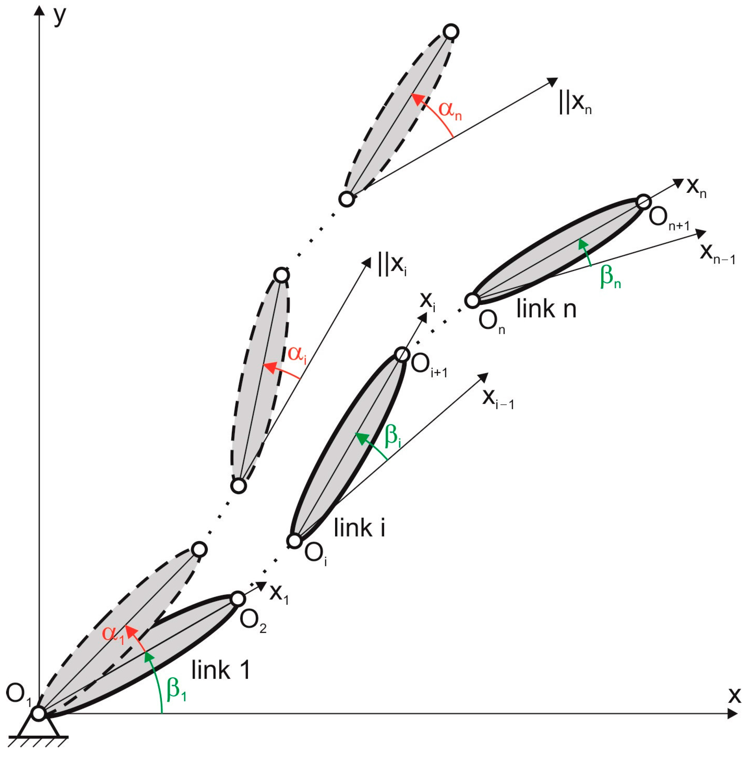
This section deals with the mathematical model of the robot that describes low-frequency vibrations. These vibrations are due to the flexibility of the joints and consist of the rotational oscillations of the links relative to the joints. In order to take them into account, it can be assumed that each configuration coordinate of the arm $q_i$ can be expressed as the sum of two angular values:

$$q_i={\beta }_i+{\alpha }_i,$$

(1)

where ${\beta }_i$ is a variable describing the position of the i-th link of the manipulator, relative to which the oscillations of this element, expressed by the variable ${\alpha }_i$, take place (Figure 1). In the ideal case, when there are no vibrations, ${\beta }_i$ is identical to the configuration coordinate $q_i$. If there is compliance in the joints, the angle ${\alpha }_i$ is a rapidly changing value related to vibration phenomena. On the other hand, ${\beta }_i$ is a slowly changing value whose change results from the execution of the motion path, or it can be a constant value if the link is in a fixed position.

Since the present research is concerned with vibration phenomena and not with the overall movement of the arm, a simplifying assumption was made in further considerations. The vibrational movements of the elements described by the ${\alpha }_i$ variables were considered in relation to the positions of the elements described by the ${\beta }_i$ coordinates, which were treated as constants. In other words, the vibrations of the kinematic chain relative to the assumed position defined by the ${\beta }_i$ coordinates are the subject of the analysis. This approach is justified by the fact that, during the movement, changes in ${\beta }_i$ are many times slower than changes in ${\alpha }_i$. Therefore, based on Equation (1), the angular velocities of the elements are expressed as follows:

$${\dot{q}}_i={\dot{\alpha }}_i$$

(2)

The equation describing the vibrations of the robot in the selected arm position, in the case without constraints, can be written in the following form:

$$\mathit{M}\left(\mathit{\alpha },\mathit{\beta }\right)\ddot{\mathit{\alpha }}+\mathit{C}\left(\mathit{\alpha },\dot{\mathit{\alpha }},\mathit{\beta }\right)\dot{\mathit{\alpha }}+\mathit{D}\dot{\mathit{\alpha }}+\mathit{K}\mathit{\alpha }=\mathit{u}+{\mathit{\tau }}_{ext},$$

(3)

where $\mathit{\alpha }\in {\mathit{R}}^n$—a vector of coordinates representing the vibrations of the links of the robot, such that $\mathit{\alpha }={\left[\begin{array}{ccccc}{\alpha }_1& \dots & {\alpha }_i& \dots & {\alpha }_n\end{array}\right]}^T$; $\mathit{\beta }=\mathit{c}\mathit{o}\mathit{n}\mathit{s}\mathit{t}.\in {\mathit{R}}^n$—a vector of coordinates representing the position of the robot arm, such that $\mathit{\beta }={\left[\begin{array}{ccccc}{\beta }_1& \dots & {\beta }_i& \dots & {\beta }_n\end{array}\right]}^T$; $\mathit{M}\left(\mathit{\alpha },\mathit{\beta }\right)\in {\mathit{R}}^{n\times n}$—an inertia matrix; $\mathit{C}\left(\mathit{\alpha },\dot{\mathit{\alpha }},\mathit{\beta }\right)\dot{\mathit{\alpha }}\in {\mathit{R}}^n$—a vector of centrifugal and Coriolis forces (moments of forces); $\mathit{D}\in {\mathit{R}}^{n\times n}$—a matrix of joints damping; $\mathit{K}\in {\mathit{R}}^{n\times n}$—a matrix of joint stiffness; $\mathit{u}\in {\mathit{R}}^n$—a control input vector; ${\mathit{\tau }}_{ext}\in {\mathit{R}}^n$—an external excitation vector. Equation (3) is a system of second-order nonlinear coupled differential equations.

Equation (3) defines the general structure of the dynamics equations describing the vibrations of the links relative to the configuration defined by the $\mathit{\beta }$ vector. The equation of motion of the robot arm in the form (3) for the selected robot can be obtained using various mathematical formalisms. The remainder of this section presents an approach based on the Lagrange formalism for a fragment of an industrial robot arm with two degrees of freedom. Detailed derivations of the equations of motion are presented in [30], where a mathematical model is presented without taking into account viscous damping and an excitation vector. For this reason, this article is limited to presenting the most important information about the mathematical model of the robot arm with two degrees of freedom.

The manipulator diagram is shown in Figure 2. The model takes into account the compliance of the joints at points A and B. The stiffness of the joints at points A and B are represented by the coefficients $k_1$ and $k_2$, respectively. The viscous damping coefficients in the joints are $d_1$ and $d_2$. The lengths of links 1 and 2 are $l_1$ and $l_2$, respectively. The masses of the links are $m_1$ and $m_2$, respectively, the moment of inertia of link 1 relative to point A is $I_A^{\left(1\right)}$ and the moment of inertia of link 2 relative to point S₂ is $I_{S2}^{\left(2\right)}$. Points S₁ and S₂ are the centres of mass of the links, defined relative to joints A and B by the values $l_{c1}$ and $l_{c2}$, respectively. The moments that cause the arm to vibrate are $u_1$ and $u_1$, and $F_{ext}$ is an external force vector.

The equations of motion of the manipulator were formulated using the Lagrange formalism, based on the following system of equations:

$$\frac{d}{dt}\left(\frac{\partial L}{\partial {\dot{\alpha }}_i}\right)-\frac{\partial L}{\partial {\alpha }_i}=Q_i,$$

(4)

where $L=E-V$ is the Lagrange function, which is the difference between kinetic and potential energy and $Q_i$ is generalised force.

The potential energy of the system is the sum of the potential energy of the masses of the links $V_{g1}$ and $V_{g2}$ and the potential energy of the elastic joints $V_{k1}$ and $V_{k2}$:

$$V=V_{k1}+V_{k2}+V_{g1}+V_{g2},$$

(5)

where

$$V_{k1}=\frac{1}{2}{k}_1{\left({\alpha }_1+{\alpha }_{1st}\right)}^2,$$

(6)

$$V_{k2}=\frac{1}{2}{k}_2{\left({\alpha }_2+{\alpha }_{2st}\right)}^2,$$

(7)

$$V_{g1}=m_{1}g{l}_{c1}\sin \left({\beta }_1+{\alpha }_1\right),$$

(8)

$$V_{g2}=m_{2}g\left[l_1\sin \left({\beta }_1+{\alpha }_1\right)+l_{c2}\sin \left({\beta }_1+{\beta }_2+{\alpha }_1+{\alpha }_2\right)\right],$$

(9)

where ${\alpha }_{1st}$ and ${\alpha }_{2st}$ represent static deformations of joints under the influence of moments resulting from the gravitational forces of the joints. Expansions of the type $\sin \left(a+b\right)=\sin a\cos b+\cos a\sin b$ were applied to the sines of the sums of the angles appearing in Equations (8) and (9). Maintaining the assumption that the angular coordinates ${\alpha }_1$ and ${\alpha }_2$ describing vibrations have small values, it was assumed that $\sin {\alpha }_1={\alpha }_1$, $\cos {\alpha }_1=1$, $\sin \left({\alpha }_1+{\alpha }_2\right)={\alpha }_1+{\alpha }_2$ and $\cos \left({\alpha }_1+{\alpha }_2\right)=1$. Then, using the Dirichlet criterion, the static deformations of the joints that occur in the static equilibrium position in conditions where ${\alpha }_1={\alpha }_2=0$ were determined. Taking into account the static deformations and ignoring ${\alpha }_{1st}^2$ and ${\alpha }_{2st}^2$ as small values of higher order than ${\alpha }_{1st}$ and ${\alpha }_{2st}$, the potential energy was obtained in the following form:

$$V=\frac{1}{2}{k}_1{\alpha }_1^2+\frac{1}{2}{k}_2{\alpha }_2^2+m_{1}g{l}_{c1}\sin {\beta }_1+m_{2}g{l}_1\sin {\beta }_1+m_{2}g{l}_{c2}\sin \left({\beta }_1+{\beta }_2\right).$$

(10)

The kinetic energy of the system is the sum of the kinetic energy of link 1 in rotation and link 2 in plane motion:

$$E=\frac{1}{2}{I}_A^{\left(1\right)}{\dot{q}}_1^2+\frac{1}{2}{m}_2{v}_{S2}^2+\frac{1}{2}{I}_{S2}^{\left(2\right)}{\left({\dot{q}}_1+{\dot{q}}_2\right)}^2,$$

(11)

where $v_{S2}$ is the velocity of the centre of mass of link 2. Its value was defined as $v_{S2}=\sqrt{{\dot{x}}_{S2}^2+{\dot{y}}_{S2}^2}$, where the velocity components are derivatives of the coordinates of point S₂ in the xy coordinate system, given by the following system of equations:

$$\{\begin{array}{c}{x}_{S2}=l_1\cos \left(q_1\right)+l_{c2}\cos \left(q_1+q_2\right)\\ y_{S2}=l_1\sin \left(q_1\right)+l_{c2}\sin \left(q_1+q_2\right)\end{array}.$$

(12)

taking into account Equations (1) and (2) in the kinematics Equation (12), an equation determining the kinetic energy of the system was obtained in the following form:

$$\begin{array}{c}E=\frac{1}{2}\left[I_A^{\left(1\right)}+I_{S2}^{\left(2\right)}+m_2{l}_1^2+m_2{l}_{c2}^2+m_2{l}_1{l}_{c2}\cos \left({\beta }_2+{\alpha }_2\right)\right]{\dot{\alpha }}_1^2+[m_2{l}_{c2}^2+\\ m_2{l}_1{l}_{c2}\cos \left({\beta }_2+{\alpha }_2\right)+I_{S2}^{\left(2\right)}]{\dot{\alpha }}_1{\dot{\alpha }}_2+\frac{1}{2}\left(m_2{l}_{c2}^2+I_{S2}^{\left(2\right)}\right){\dot{\alpha }}_2^2.\end{array}$$

(13)

the generalised forces were determined using the principle of virtual work. The virtual work of nonpotential forces $dW$ is equal to virtual work of generalized force $Q_{i}d{\alpha }_i$, so

$$dW=F_{i}d{\alpha }_i-\frac{\partial R}{\partial {\dot{\alpha }}_i}d{\alpha }_i=Q_{i}d{\alpha }_i.$$

(14)

where $F_i$—external forces for link $i$; $R$—energy dissipation function; $i=1,2$. The energy dissipation function is given in the following form:

$$R=\frac{1}{2}{d}_1{\dot{\alpha }}_1^2+\frac{1}{2}{d}_2{\dot{\alpha }}_2^2.$$

(15)

the external force is as follows:

$$F_i=u_i+{\tau }_{ext i}.$$

(16)

where $u_i$—control input for link $i$; ${\tau }_{ext i}$—the torque of any forces acting on the end-effector of the robot. Taking into account Equations (14)–(16), the generalized force $Q_i$ is written as follows

$$Q_i=u_i+{\tau }_{ext i}-d_i{\dot{\alpha }}_i^2.$$

(17)

using Equation (4), the equations of motion of the system were obtained in the general form of Equation (3), where the vectors and matrices have the following form:

$$\mathit{\alpha }=\left[\begin{array}{c}{\alpha }_1\\ {\alpha }_2\end{array}\right],$$

(18)

$$\mathit{M}\left(\mathit{\alpha },\mathit{\beta }\right)=\left[\begin{array}{cc}{a}_1+2a_2\cos \left({\beta }_2+{\alpha }_2\right)& a_3+a_2\cos \left({\beta }_2+{\alpha }_2\right)\\ a_3+a_2\cos \left({\beta }_2+{\alpha }_2\right)& a_3\end{array}\right],$$

(19)

$$\mathit{C}\left(\mathit{\alpha },\dot{\mathit{\alpha }},\mathit{\beta }\right)=\left[\begin{array}{cc}-a_2\sin \left({\beta }_2+{\alpha }_2\right){\dot{\alpha }}_2& -a_2\sin \left({\beta }_2+{\alpha }_2\right)\left({\dot{\alpha }}_1+{\dot{\alpha }}_2\right)\\ a_2\sin \left({\beta }_2+{\alpha }_2\right){\dot{\alpha }}_1& 0\end{array}\right],$$

(20)

$$\mathit{D}=\left[\begin{array}{cc}{d}_1& 0\\ 0& d_2\end{array}\right],$$

(21)

$$\mathit{K}=\left[\begin{array}{cc}{k}_1& 0\\ 0& k_2\end{array}\right],$$

(22)

$$\mathit{u}=\left[\begin{array}{c}{u}_1\\ u_2\end{array}\right],$$

(23)

$${\mathit{\tau }}_{ext}=\left[\begin{array}{c}{\tau }_{ext 1}\\ {\tau }_{ext 2}\end{array}\right]={\mathit{J}}_a^T\left(\mathit{\alpha },\mathit{\beta }\right){\mathit{F}}_{ext}.$$

(24)

the $a_i$ parameters result from the following coefficients:

$$\{\begin{array}{c}{a}_1=I_A^{\left(1\right)}+I_{S2}^{\left(2\right)}+m_2{l}_1^2+m_2{l}_{c2}^2\\ a_2=m_2{l}_1{l}_{c2}\\ a_3=I_{S2}^{\left(2\right)}+m_2{l}_{c2}^2\end{array}.$$

(25)

the values of the model parameters are given in

Table 1. Coefficient values used in robot model.

Coefficient	Unit	Value
$I_A^{\left(1\right)}$	kg∙m2	0.55
$I_{S2}^{\left(2\right)}$	kg∙m2	0.0009
$m_2$	kg	50.58
$l_1$	m	0.63
$l_{c2}$	m	0.1
$k_1$	N∙m/rad	555,000
$k_2$	N∙m/rad	128,000
$d_1$	N∙m∙s/rad	0.9
$d_2$	N∙m∙s/rad	0.9

. The method for their determination is given in the paper in [30]. Equation (24) takes into account the relationship between the vector of external forces ${\mathit{F}}_{ext}$ applied to the robot end-effector and the moment of these forces ${\mathit{\tau }}_{ext}$ acting on the robot’s links using the analytical Jacobian ${\mathit{J}}_a\left(\mathit{\alpha },\mathit{\beta }\right)$. Since the kinematic relationship between the coordinates of the robot end-effector (point C) and the angular coordinates is given by the system of equations

$$\{\begin{array}{c}{x}_C=l_1\cos \left({\beta }_1+{\alpha }_1\right)+l_2\cos \left({\beta }_1+{\beta }_2+{\alpha }_1+{\alpha }_2\right)\\ y_C=l_1\sin \left({\beta }_1+{\alpha }_1\right)+l_2\sin \left({\beta }_1+{\beta }_2+{\alpha }_1+{\alpha }_2\right)\end{array},$$

(26)

the analytical Jacobian has the following form:

$${\mathit{J}}_a\left(\mathit{\alpha },\mathit{\beta }\right)=\left[\begin{array}{cc}-l_1\sin \left({\beta }_1+{\alpha }_1\right)-l_2\sin \left({\beta }_1+{\beta }_2+{\alpha }_1+{\alpha }_2\right)& -l_2\sin \left({\beta }_1+{\beta }_2+{\alpha }_1+{\alpha }_2\right)\\ l_1\cos \left({\beta }_1+{\alpha }_1\right)+l_2\cos \left({\beta }_1+{\beta }_2+{\alpha }_1+{\alpha }_2\right)& l_2\cos \left({\beta }_1+{\beta }_2+{\alpha }_1+{\alpha }_2\right)\end{array}\right].$$

(27)

The mathematical model is used for the analysis, the results of which are presented in Section 3 and Section 4.

3. Natural Vibrations of a Linear System

Occasionally, publications on robot vibrations present resonance curves that show the dependence of the resonance frequencies on the position of the robot arm [31,32]. They are prepared on the basis of modal experiments in which the vibration is excited by an impact hammer pulse. The robot in the selected position is treated as a linear object; thus, bifurcation phenomena are not analysed. In order to be able to compare nonlinear models with such basic analyses, simplified robot motion equations were first considered. The influence of nonlinear elements, damping and excitation was ignored in order to determine the natural frequencies of the arm in selected configurations. Therefore, taking into account the above-mentioned simplifications, Equation (3) was reduced to the following form:

$$\mathit{M}\left(\mathit{\alpha },\mathit{\beta }\right)\ddot{\mathit{\alpha }}+\mathit{K}\mathit{\alpha }=0.$$

(28)

as indicated in [30], the natural frequencies of the arm can be determined from the following equation:

$$det\left(-{\omega }_0^2{\mathit{M}}_0+\mathit{K}\right)=0$$

(29)

where ${\omega }_0$—natural frequency of the robot; ${\mathit{M}}_0=\mathit{M}\left(\mathit{\alpha }=\mathbf{0},\mathit{\beta }\right)$—an inertia matrix in which the influence of the ${\alpha }_i$ angles is neglected and which is constant at a given position of the arm defined by the coordinate vector $\mathit{\beta }$. Taking into account the forms of the inertia and stiffness matrices defined by Equations (19) and (22), the following two natural frequencies (${\omega }_{0\left\{1\right\}}$ and ${\omega }_{0\left\{2\right\}}$) of the robot arm were determined:

$${\omega }_{0\left\{1,2\right\}}=\sqrt{\frac{\left(a_1{k}_2+2a_2{k}_2\cos {\beta }_2+a_3{k}_1\right)\mp \sqrt{{\left(a_1{k}_2+2a_2{k}_2\cos {\beta }_2+a_3{k}_1\right)}^2-4\left(a_1{a}_3-a_3^2-a_2^2{\cos }^2{\beta }_2\right)k_1{k}_2}}{2\left(a_1{a}_3-a_3^2-a_2^2{\cos }^2{\beta }_2\right)}}.$$

(30)

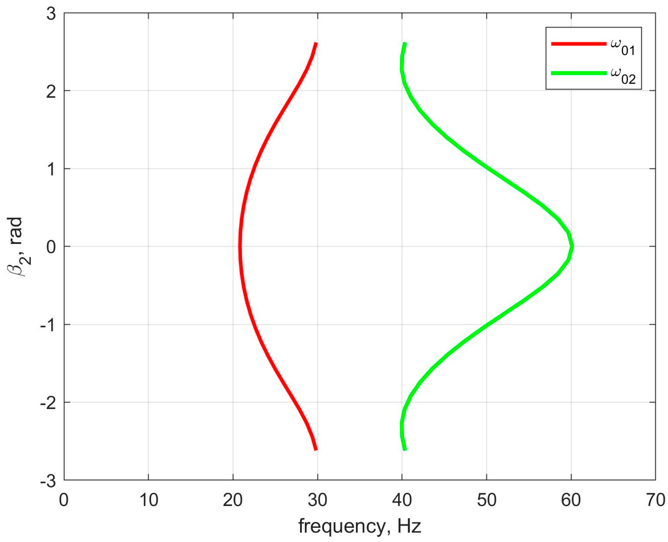
it is clear from solution (30) that the natural frequencies depend on the position of link 2 relative to link 1, expressed by the angle ${\beta }_2$. The dependence of the natural frequencies on the angle ${\beta }_2$ is shown in Figure 3. In addition, the natural frequencies are expressed in Hz using the transformation $f_{0\left\{1,2\right\}}={\omega }_{0\left\{1,2\right\}}/\left(2\pi \right)$.

The natural frequencies of the robot arm vibrations depend strongly on its position, and the changes are symmetrical with respect to the so-called straight arm configuration (${\beta }_2=0$). The simulation results are in agreement with the results of the experimental research presented in [30]. On this basis, it can be assumed that the mathematical model has suitable properties for simulation studies of vibration phenomena.

4. Bifurcation Analysis of Forced Vibrations

Firstly, the simulation results of the influence of the forcing frequency as a bifurcation parameter on the vibration characteristics are presented. The calculations were carried out using “Matcont 7.4” software [33,34]. The research used a mathematical model given by Equation (3), taking into account Equations (18)–(25) and (27) and the parameters given in Table 1. The following forcing vector was used:

$$\mathit{u}=\left[\begin{array}{c}{u}_{e1}\sin \left(2\pi f_{e1}t\right)\\ 0\end{array}\right],$$

(31)

where $u_{e1}$—forcing amplitude for link 1; $f_{e1}$—forcing frequency for link 1. During the tests, the forced vibrations of the system were analysed at a variable forcing frequency in the range of $f_{e1}\in \langle 0,80\rangle$ Hz. As the direction of the change in the frequency value affects the behaviour of the system, tests were carried out for increasing and decreasing frequencies (so called forward and backward sweep). In this case, the vector of external forces ${\mathit{F}}_{ext}$ is equal to 0. The tests were carried out for many arm configurations defined by the angle ${\beta }_2\in \langle 0,150\rangle$ deg. The obtained amplitude–frequency characteristics of link 1 for selected positions of the robot arm are shown in Figure 4. Figure 4a shows the amplitude–frequency characteristics for the angle ${\beta }_2$ of 0 rad (0 deg), 0.5236 rad (30 deg), 1.0472 rad (60 deg), 1.5708 rad (90 deg), 2.0944 rad (120 deg) and 2.6180 rad (150 deg), with areas of instability marked by a red line. The graphs show that, similar to the natural frequencies in a linear system (Section 3), in a nonlinear system the resonance zones move closer together as the absolute value of angle ${\beta }_2$ increases. In addition, the phenomenon of the dependence of the vibration amplitude on the direction of the frequency change is visible, resulting in a slope of the characteristics in the resonance zones. For small ${\beta }_2$ angles, a stiff resonance curve is obtained around the first natural frequency (Figure 4b), which for large ${\beta }_2$ transits into a mixed softening–hardening curve. In contrast, for the resonance around the second natural frequency (Figure 4c), soft characteristics are obtained. As the angle ${\beta }_2$ increases, the situation changes: the curves shift towards lower frequencies and become stiff characteristics.

In the range of negative values of ${\beta }_2$, the characteristics are identical to those for positive values; therefore, the results for the angle ${\beta }_2<0$ are not presented. This is physically justified, as from the point of view of the behaviour of the dynamic system it does not matter whether the arm configuration is “elbow up” or “elbow down”. In addition, the characteristics for link 2 are qualitatively identical to the characteristics for link 1 shown in Figure 4 and are therefore not included in this paper.

The influence of the forcing amplitude as a bifurcation parameter on the vibration characteristics was also investigated. The tests used the forcing vector in the form of Equation (25) and assumed the forcing frequency $f_{e1}=22.5$ Hz and a variable forcing amplitude. The tests were carried out for selected arm configurations defined by the ${\beta }_2$ angle.

Figure 5 shows selected results obtained for the selected forcing frequency and various arm positions. The characteristics show that the oscillations of the link can have different amplitudes depending on the forcing amplitude. The areas shown with red lines are areas of instability.

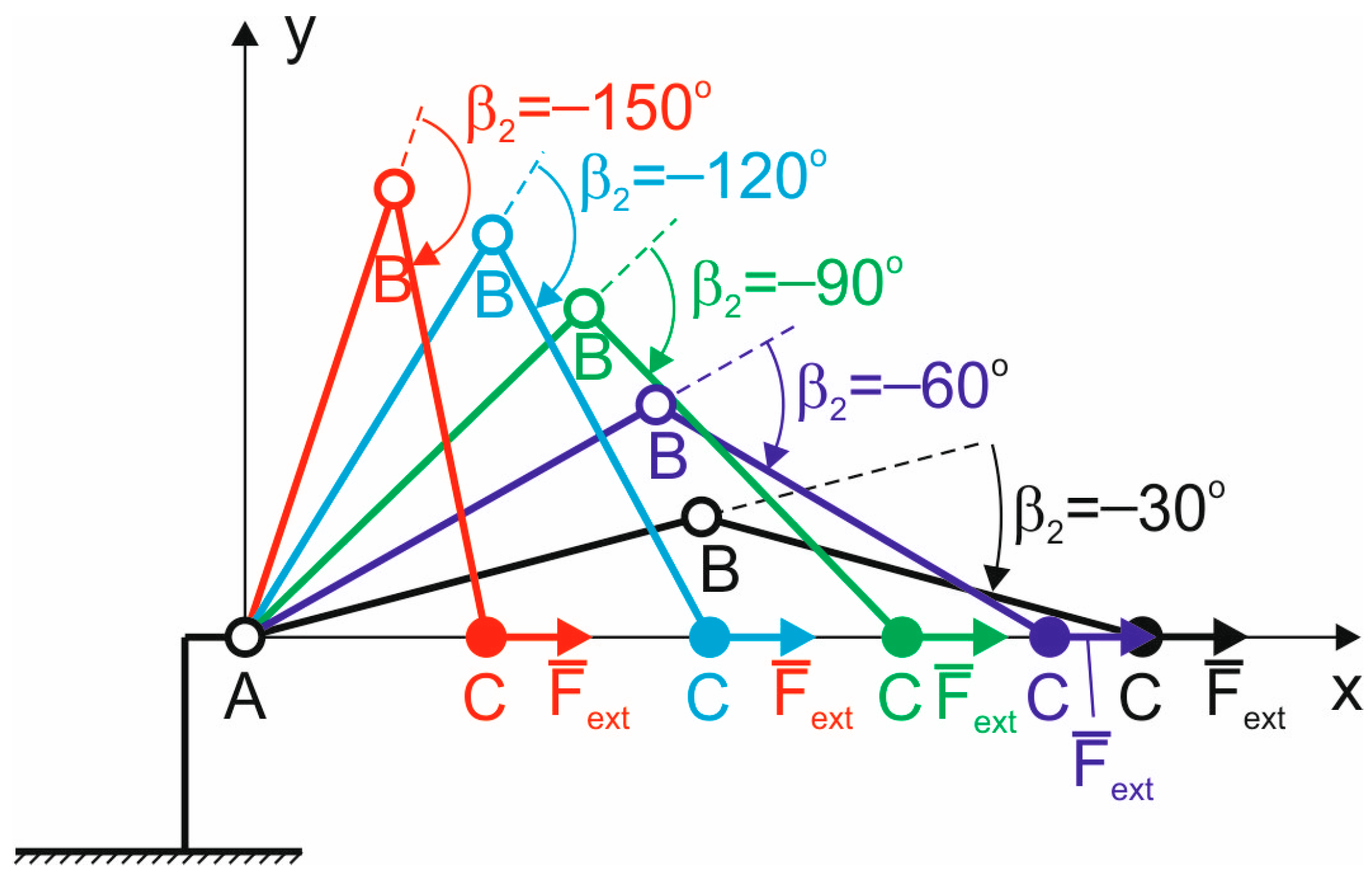
In the next study, the characteristics of the system were determined in the case of a force applied to the end-effector of the robot. It was assumed that the end-effector takes successive positions on a straight line parallel to the x axis (Figure 6). A harmonic excitation was applied with a direction parallel to the x axis:

$${\mathit{F}}_{ext}=\left[\begin{array}{c}{F}_{ext\_x}\sin \left(2\pi f_{x}t\right)\\ 0\end{array}\right],$$

(32)

where $F_{ext\_x}$—forcing amplitude in $x$ direction; $f_x$—forcing frequency. During the tests, the forced vibrations of the system were analysed at a variable forcing frequency in the range of $f_x\in \langle 0,80\rangle$ Hz. Despite the constant amplitude $F_{ext\_x}$ of the force, its effect depends on the position of the robot, because the moment of this force acting on the links depends on ${\beta }_1$ and ${\beta }_2$. Moreover, it was assumed that the control input vector $\mathit{u}$ is equal to 0. The remaining conditions were the same as in the previously discussed simulation study. The simulation case discussed approximates the conditions of robotic machining of flat surfaces or edges, where the robot tip moves along a straight line. The harmonic force approximates the dynamic component of the cutting force acting on the robot.

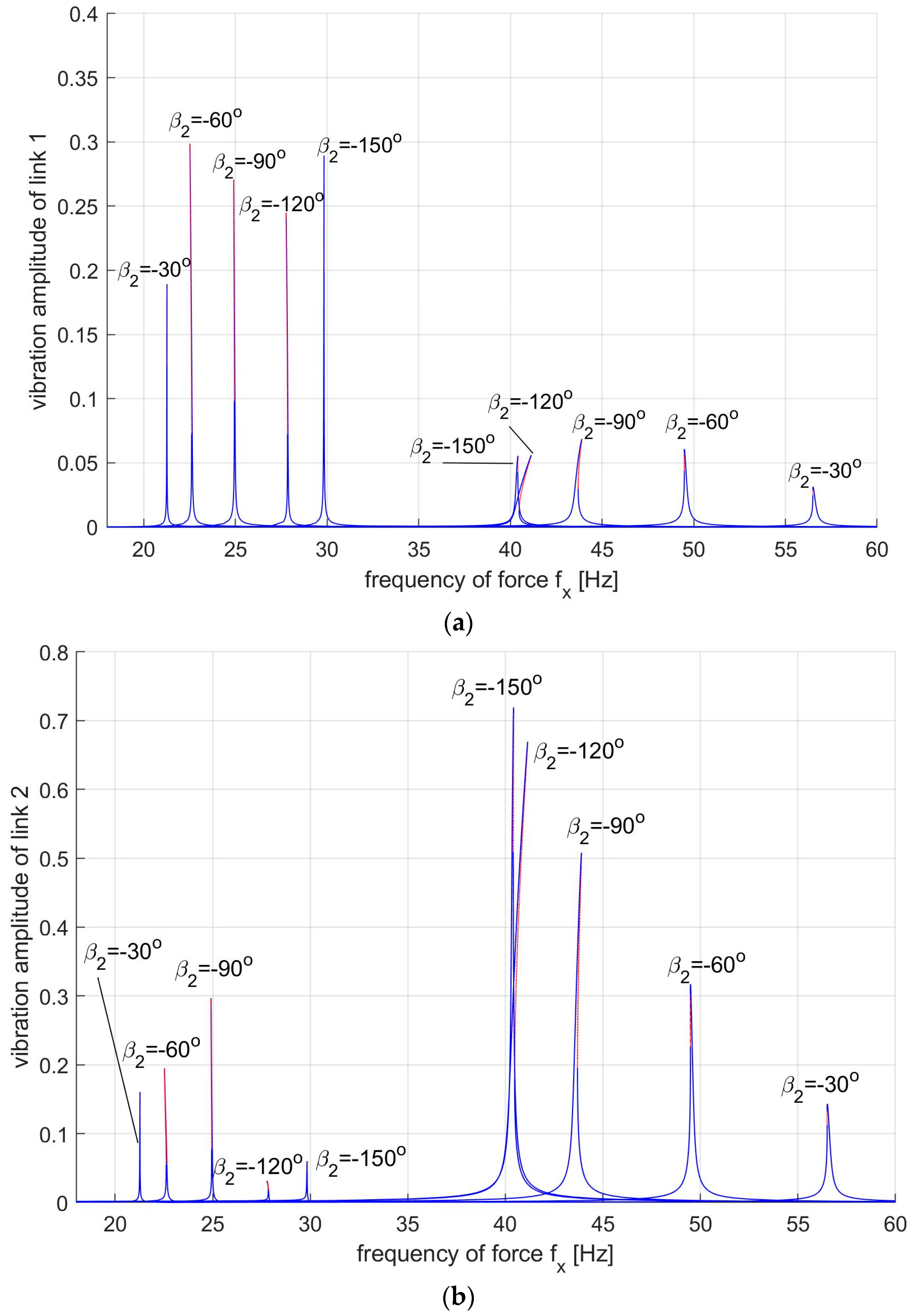
The results of the analysis are shown in Figure 7. Figure 7a shows the amplitude–frequency characteristics for element 1 at selected positions presented in Figure 6. Figure 7b shows the characteristics for element 2.

The vibration amplitudes of the first link are significantly greater in the first resonance zone than in the second zone, while the opposite is true for element 2. As for the phenomenon of the slope of the characteristics, it is more clearly visible in the second resonance zone for both elements. Figure 7c,d also show the influence of the external force amplitude on the characteristics in the selected arm position. As a result of the increase in force amplitude, not only does the vibration amplitude increase, but the nonlinear effects are also amplified. Figure 7c shows that as a result of the simultaneous slope of the characteristic and the increase in vibration amplitude, there is a significant widening of the second resonance zone. However, Figure 7d shows a more complex part of the characteristic in the first resonance zone, namely that as the excitation amplitude increases, two maxima appear and the resonance zone widens.

5. Experimental Studies

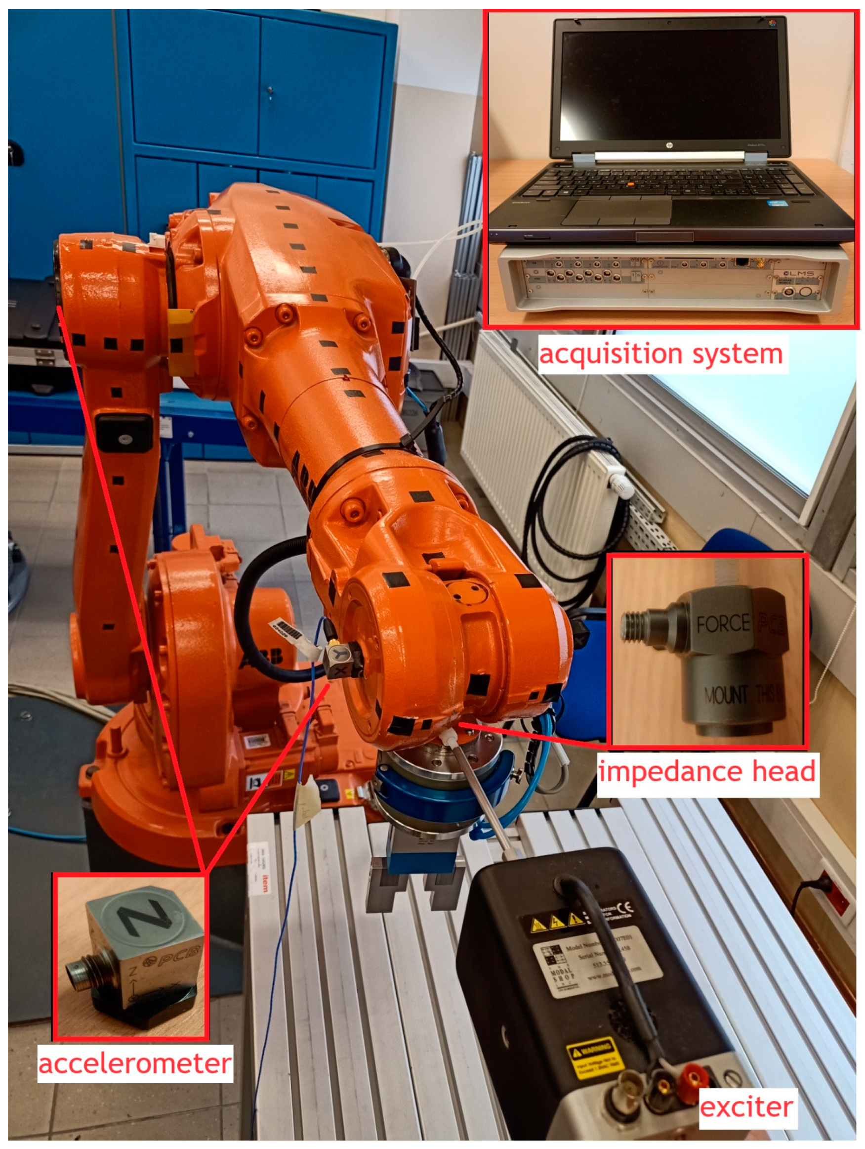
To verify the accuracy of the mathematical model, experimental tests were carried out using the test stand shown in Figure 8. The stand included the ABB IRB 1600 robot (ABB Ltd., Zürich, Switzerland), an electrodynamic exciter, an impedance head, a set of vibration sensors, an LMS Scadas mobile recorder (LMS International, Leuven, Belgium) and LMS Test.Xpress 5a software (LMS International, Leuven, Belgium). The tests used the functionality of the LMS Test.Xpress 5a software, which has the ability to control the exciter in a loop with feedback based on force measurement using an impedance head. A set of accelerometers attached to the manipulator joints (points B and C, Figure 6) was used to measure the vibrations of the robot. The acceleration signals were integrated twice to obtain the point displacements, and then the angular displacements of the links were calculated using the kinematics equations.

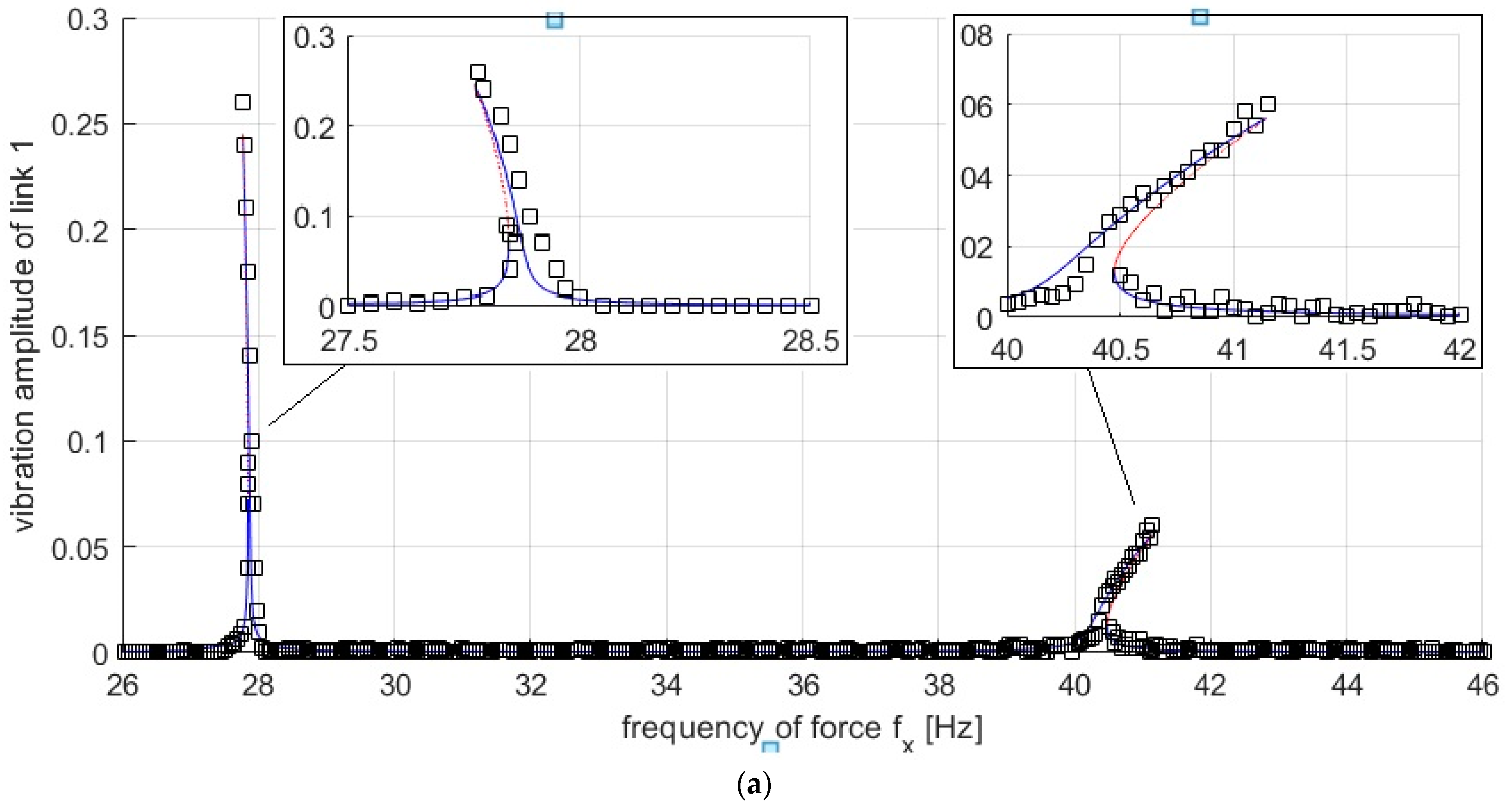
The tests were carried out in one of the robot positions shown in Figure 6, for ${\beta }_2=-120$ deg. The excitation described by Equation (32) was used, where the excitation frequency was variable in the range 26–46 Hz in order to excite resonant vibrations in the robot in the two expected resonance zones. The characteristics obtained are shown in Figure 9. In order to compare the characteristics obtained, the results of the simulation (solid line) and the experiment (square markers) are shown simultaneously.

Figure 9 shows the phenomena predicted in the simulation tests, i.e., in the first resonance zone there are soft resonance curves, while in the second resonance zone there are stiff resonance curves. There are slight differences between the simulation and experimental results, e.g., for link 1 in the first resonance zone slightly higher amplitude values were obtained in the experimental tests (Figure 9a), while for link 2 in the second resonance zone the actual vibration amplitudes were slightly smaller than those predicted in the simulation (Figure 9b). As for the first resonance zone for link 2, the vibration amplitudes are so small that it is difficult to observe a clear nonlinear effect. Only in the context of the knowledge obtained from the simulation of a mathematical model is it easier to interpret the experimental results, and a slight slope of the characteristics can be observed.

6. Conclusions and Discussion

The results presented in this paper concern the study of the influence of two parameters on the behaviour of a nonlinear dynamic system such as an industrial robot arm. Based on the tests of the mathematical model, which was confirmed through the results of the experimental tests, a nonlinear dependence of the vibration amplitude of the links on both the frequency and the amplitude of the excitation was demonstrated. On the basis of the tests carried out, it was found that the vibration amplitude of the links depends nonlinearly on the amplitude of the harmonic excitation and that there are bifurcation points whose location depends on the position of the arm described by the angle ${\beta }_2$. In the case of the amplitude–frequency characteristics, the dependence of the resonance zones on the position of the arm was demonstrated, and the resonance characteristics changed from stiff to soft or vice versa. In addition, within the resonant zones there are instability areas. In these areas, the vibration amplitudes depend on the direction of changes in the forcing frequency, and the amplitude values can vary by up to six times depending on the direction of changes in the forcing frequency. In addition, for larger excitation amplitudes, period doubling, saddle-node points and Neimark–Sacker bifurcation were observed but are not indicated in this paper as they require a separate detailed analysis.

In the context of the existing literature, it can be stated that the analysis of the vibrations of industrial robots usually uses the approach for linear systems, where the frequency response function is used to determine the amplitude–frequency characteristics. The nonlinear vibration effects of robot arms presented in this article are not taken into account when creating robot models. This clearly shows that treating an industrial robot arm as a linear system is only a simplification and can lead to significant errors in the solutions obtained.

Experimental tests carried out using an external system that induces vibrations in the robot with a harmonic force reflect the operating conditions, for example in the mechanical machining process, where dynamic, periodically variable forces of high values (from a few to several hundred Newtons, depending on the type of machining) act on the robot arm. In this context, the research results presented illustrate the dynamic phenomena that can occur in robotic machining processes. Due to nonlinear phenomena, the resonance zones are more extensive at larger excitation amplitudes than at small amplitudes, where nonlinear phenomena have less influence on the system. This also leads to the conclusion that in order to avoid nonlinear phenomena, which are difficult to analyse and control due to areas of instability, large excitations acting on the robot should be avoided. Therefore, in mechanical machining processes, it is advantageous to use lower feed rates or lower tool pressure forces (smaller cutting depths) to reduce the dynamic forces. Unfortunately, this leads to an increase in process execution time.

As for further work in the area of the presented topic, it is planned to study the impact of holonomic constraints on the vibration phenomena of the robot. Holonomic constraints occur when the robot comes into contact with the environment, in tasks such as assembly or mechanical processing, such as grinding or polishing.