
The Optimal Erection of the Inverted Pendulum


Abstract
:1. Introduction
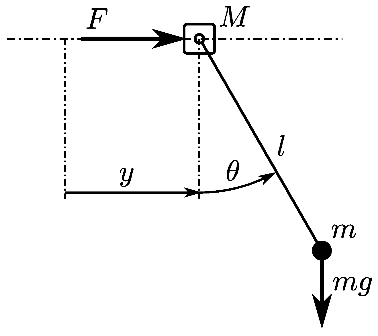
2. Dynamic Model
3. Optimal Control Problem
Singular Arc
4. Numerical Solution
4.1. Baseline
4.2. Sensitivity to
4.3. Sensitivity to Initial Conditions
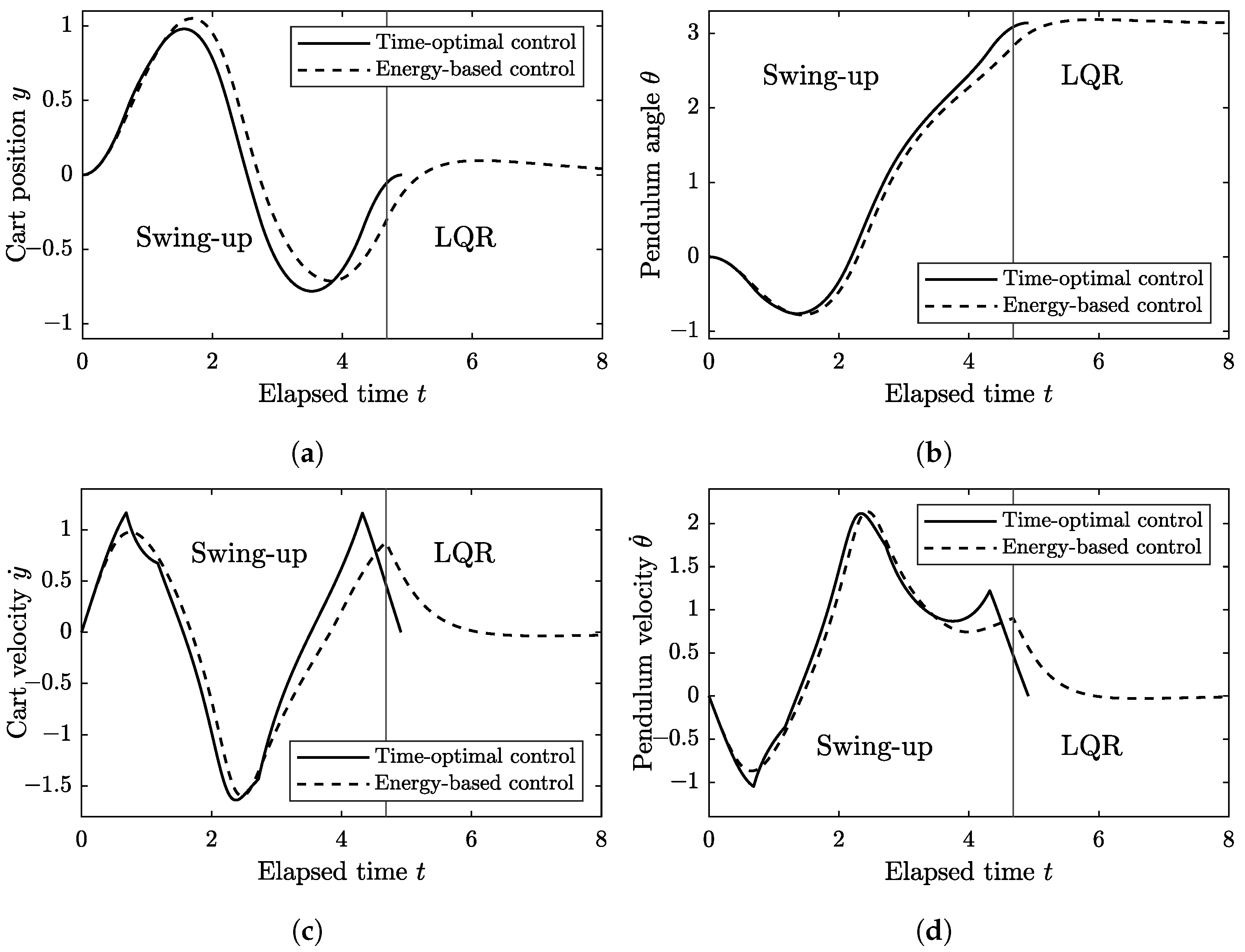
4.4. Comparison to Energy-Based Control Strategy
5. Conclusions
Author Contributions
Funding
Data Availability Statement
Conflicts of Interest
References
- Limebeer, D.J.N.; Massaro, M. Dynamics and Optimal Control of Road Vehicles; Oxford University Press: Oxford, UK, 2018. [Google Scholar]
- Sharp, R.S. On the stability and control of unicycles. Proc. R. Soc. A 2010, 466, 1849–1869. [Google Scholar] [CrossRef]
- Braghin, F.; Cheli, F.; Maldifassi, S.; Melzi, S.; Sabbioni, E. The Engineering Approach to Winter Sports; Springer: Berlin/Heidelberg, Germany, 2016. [Google Scholar]
- Hirai, K.; Hirose, M.; Haikawa, Y.; Takenaka, T. The development of Honda humanoid robot. In Proceedings of the 1998 IEEE International Conference on Robotics and Automation (Cat. No.98CH36146), Leuven, Belgium, 20 May 1998; Volume 2, pp. 1321–1326. [Google Scholar] [CrossRef]
- Hughes, P.C. Spacecraft Attitude Dynamics; Courier Corporation: Dover, UK, 2012. [Google Scholar]
- Ren, T.J.; Chen, T.C.; Chen, C.J. Motion control for a two-wheeled vehicle using a self-tuning PID controller. Control. Eng. Pract. 2008, 16, 365–375. [Google Scholar] [CrossRef]
- Prasad, L.; Tyagi, B.; Gupta, H. Optimal control of nonlinear inverted pendulum system using PID controller and LQR: Performance analysis without and with disturbance input. Int. J. Autom. Comput. 2014, 11, 661–670. [Google Scholar] [CrossRef]
- Pathak, K.; Franch, J.; Agrawal, S. Velocity and position control of a wheeled inverted pendulum by partial feedback linearization. IEEE Trans. Robot. 2005, 21, 505–513. [Google Scholar] [CrossRef]
- Anderson, C. Learning to Control an Inverted Pendulum Using Neural Networks. IEEE Control Syst. Mag. 1989, 9, 31–37. [Google Scholar] [CrossRef]
- Huang, C.H.; Wang, W.J.; Chiu, C.H. Design and Implementation of Fuzzy Control on a Two-Wheel Inverted Pendulum. IEEE Trans. Ind. Electron. 2011, 58, 2988–3001. [Google Scholar] [CrossRef]
- Huang, J.; Guan, Z.H.; Matsuno, T.; Fukuda, T.; Sekiyama, K. Sliding-mode velocity control of mobile-wheeled inverted-pendulum systems. IEEE Trans. Robot. 2010, 26, 750–758. [Google Scholar] [CrossRef]
- Balcazar, R.; Rubio, J.d.J.; Orozco, E.; Andres Cordova, D.; Ochoa, G.; Garcia, E.; Pacheco, J.; Gutierrez, G.J.; Mujica-Vargas, D.; Aguilar-Ibañez, C. The Regulation of an Electric Oven and an Inverted Pendulum. Symmetry 2022, 14, 759. [Google Scholar] [CrossRef]
- Villaseñor Rios, C.A.; Luviano-Juárez, A.; Lozada-Castillo, N.B.; Carvajal-Gámez, B.E.; Mújica-Vargas, D.; Gutiérrez-Frías, O. Flatness-Based Active Disturbance Rejection Control for a PVTOL Aircraft System with an Inverted Pendular Load. Machines 2022, 10, 595. [Google Scholar] [CrossRef]
- Yoshida, K. Swing-up control of an inverted pendulum by energy-based methods. In Proceedings of the 1999 American Control Conference (Cat. No. 99CH36251), San Diego, CA, USA, 2–4 June 1999; Volume 6, pp. 4045–4047. [Google Scholar] [CrossRef]
- Åström, K.; Furuta, K. Swinging up a pendulum by energy control. Automatica 2000, 36, 287–295. [Google Scholar] [CrossRef]
- Chatterjee, D.; Patra, A.; Joglekar, H.K. Swing-up and stabilization of a cart–pendulum system under restricted cart track length. Syst. Control. Lett. 2002, 47, 355–364. [Google Scholar] [CrossRef]
- Muskinja, N.; Tovornik, B. Swinging up and stabilization of a real inverted pendulum. IEEE Trans. Ind. Electron. 2006, 53, 631–639. [Google Scholar] [CrossRef]
- Susanto, E.; Surya Wibowo, A.; Ghiffary Rachman, E. Fuzzy Swing Up Control and Optimal State Feedback Stabilization for Self-Erecting Inverted Pendulum. IEEE Access 2020, 8, 6496–6504. [Google Scholar] [CrossRef]
- Solihin, M.I.; Wahyudi; Akmeliawati, R. Self-erecting inverted pendulum employing PSO for stabilizing and tracking controller. In Proceedings of the 2009 5th International Colloquium on Signal Processing & Its Applications, Kuala Lumpur, Malaysia, 6–8 March 2009; pp. 63–68. [Google Scholar] [CrossRef]
- Vinodh Kumar, E.; Jerome, J. Robust LQR Controller Design for Stabilizing and Trajectory Tracking of Inverted Pendulum. Procedia Eng. 2013, 64, 169–178. [Google Scholar] [CrossRef]
- Bryson, A.E. Dynamic Optimization; Addison-Wesley: Menlo Park, CA, USA, 1999. [Google Scholar]
- Mori, S.; Nishihara, H.; Furuta, K. Control of unstable mechanical system Control of pendulum†. Int. J. Control 1976, 23, 673–692. [Google Scholar] [CrossRef]
- Mason, P.; Broucke, M.E.; Piccoli, B. Time optimal swing-up of the planar pendulum. In Proceedings of the 2007 46th IEEE Conference on Decision and Control, New Orleans, LA, USA, 12–14 December 2007; pp. 5389–5394. [Google Scholar]
- Kelley, H.J.; Kopp, R.E.; Moyer, H.G. Singular extremals. In Topics in Optimization; Academic Press: Cambridge, MA, USA, 1967; Chapter 3; pp. 63–101. [Google Scholar]
- Krenner, A.J. The High Order Maximal Principle and Its Application to Singular Extremals. SIAM J. Control Optim. 1977, 15, 256–293. [Google Scholar] [CrossRef]
- Robbins, H.M. A Generalized Legendre-Clebsch Condition for the Singular Cases of Optimal Control. IBM J. 1967, 11, 361–372. [Google Scholar] [CrossRef]
- Patterson, M.A.; Rao, A.V. GPOPS-II: A Matlab Software for Solving Multiple-Phase Optimal Control Problems Using hp–Adaptive Gaussian Quadrature Collocation Methods and Sparse Nonlinear Programming. ACM Trans. Math. Softw. 2014, 41, 1–37. [Google Scholar] [CrossRef]
- Weinstein, M.J.; Rao, A.V. Algorithm 984: ADiGator, a toolbox for the algorithmic differentiation of mathematical functions in MATLAB using source transformation via operator overloading. ACM Trans. Math. Softw. 2017, 44, 1–25. [Google Scholar] [CrossRef]
- Wächter, A.; Biegler, L.T. On the Implementation of an Interior-Point Filter Line-Search Algorithm for Large-Scale Nonlinear Programming. Math. Program. 2006, 106, 25–57. [Google Scholar] [CrossRef]
- Garg, D.; Patterson, M.A.; Darby, C.L.; Francolin, C.; Huntington, G.T.; Hager, W.W.; Rao, A.V. Direct Trajectory Optimization and Costate Estimation of Finite-Horizon and Infinite-Horizon Optimal Control Problems via a Radau Pseudospectral Method. Comput. Optim. Appl. 2011, 49, 335–358. [Google Scholar] [CrossRef]
- Francolin, C.C.; Hager, W.W.; Rao, A.V. Costate Approximation in Optimal Control Using Integral Gaussian Quadrature Collocation Methods. Optim. Control Appl. Methods 2014, 36, 381–397. [Google Scholar] [CrossRef]
- Massaro, M.; Limebeer, D.J.N. Minimum-lap time simulation and optimization. Veh. Syst. Dyn. 2021, 59, 1069–1113. [Google Scholar] [CrossRef]
- Goldstein, H.; Poole, C.; Safko, J. Classical Mechanics, 3rd ed.; Pearson Education International: London, UK, 2002. [Google Scholar]


Publisher’s Note: MDPI stays neutral with regard to jurisdictional claims in published maps and institutional affiliations. |
© 2022 by the authors. Licensee MDPI, Basel, Switzerland. This article is an open access article distributed under the terms and conditions of the Creative Commons Attribution (CC BY) license (https://creativecommons.org/licenses/by/4.0/).
Share and Cite
Massaro, M.; Lovato, S.; Limebeer, D.J.N. The Optimal Erection of the Inverted Pendulum. Appl. Sci. 2022, 12, 8112. https://doi.org/10.3390/app12168112
Massaro M, Lovato S, Limebeer DJN. The Optimal Erection of the Inverted Pendulum. Applied Sciences. 2022; 12(16):8112. https://doi.org/10.3390/app12168112
Chicago/Turabian StyleMassaro, Matteo, Stefano Lovato, and David J. N. Limebeer. 2022. "The Optimal Erection of the Inverted Pendulum" Applied Sciences 12, no. 16: 8112. https://doi.org/10.3390/app12168112