
Adversarial Example Detection and Restoration Defensive Framework for Signal Intelligent Recognition Networks

Abstract
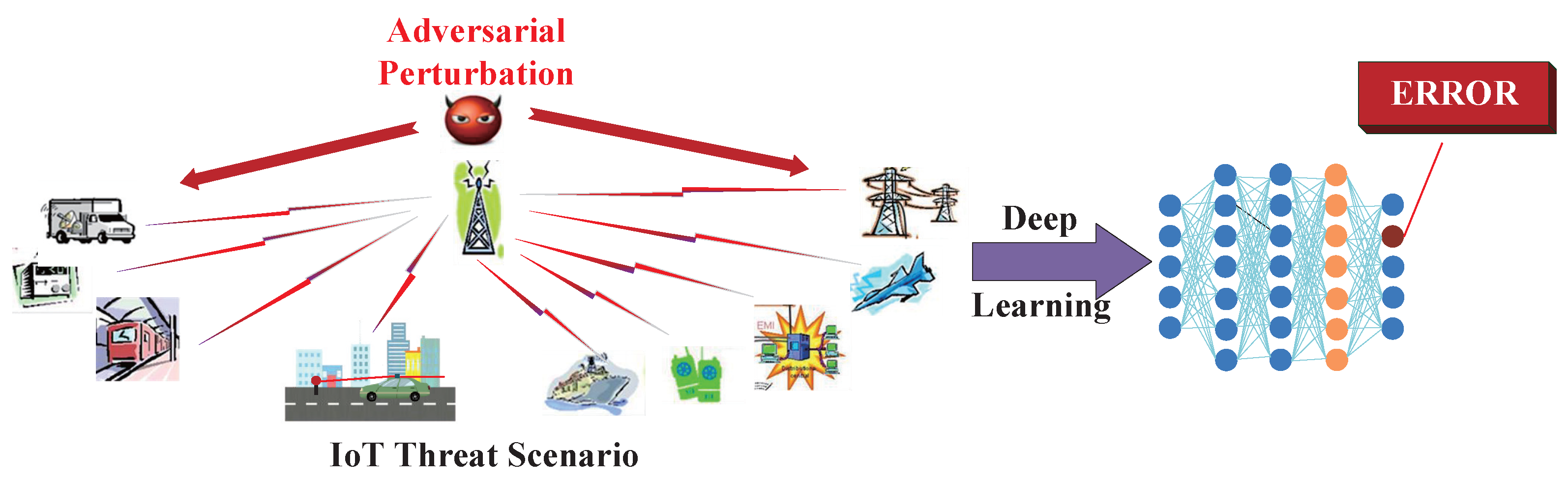
:1. Introduction
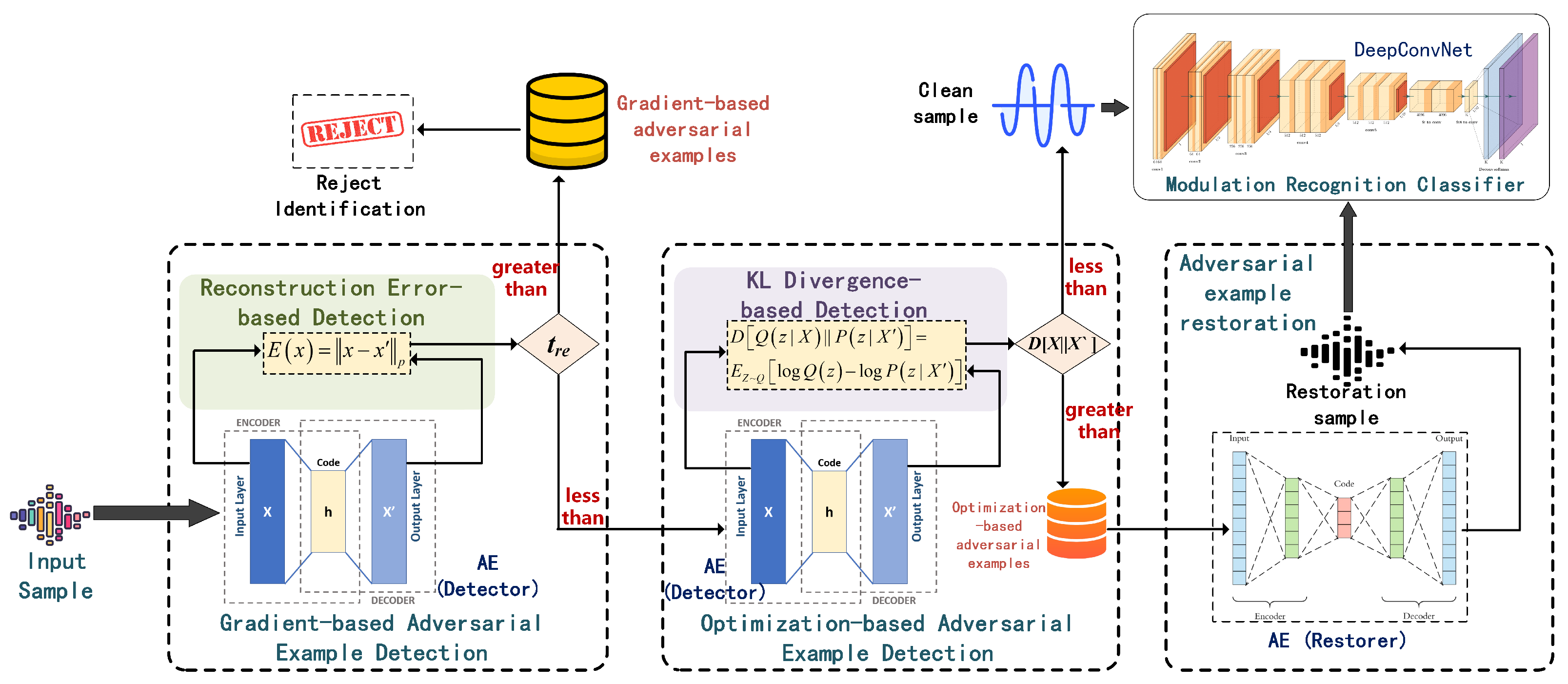
- Integrating the metrics of reconstruction error and KL divergence, we propose a refined signal adversarial example detection framework based on AE. This approach uniquely captures the deep features of input samples, marking the first-time identification of the mechanisms behind adversarial examples, discerning whether they stem from gradient-based methods or optimization techniques.
- We design an adversarial examples restoration method based on AE. Through a carefully conceived AE architecture, we effectively restored the identified adversarial examples generated through optimization techniques, thereby enhancing the model’s ability to recognize and recover from adversarial perturbations.
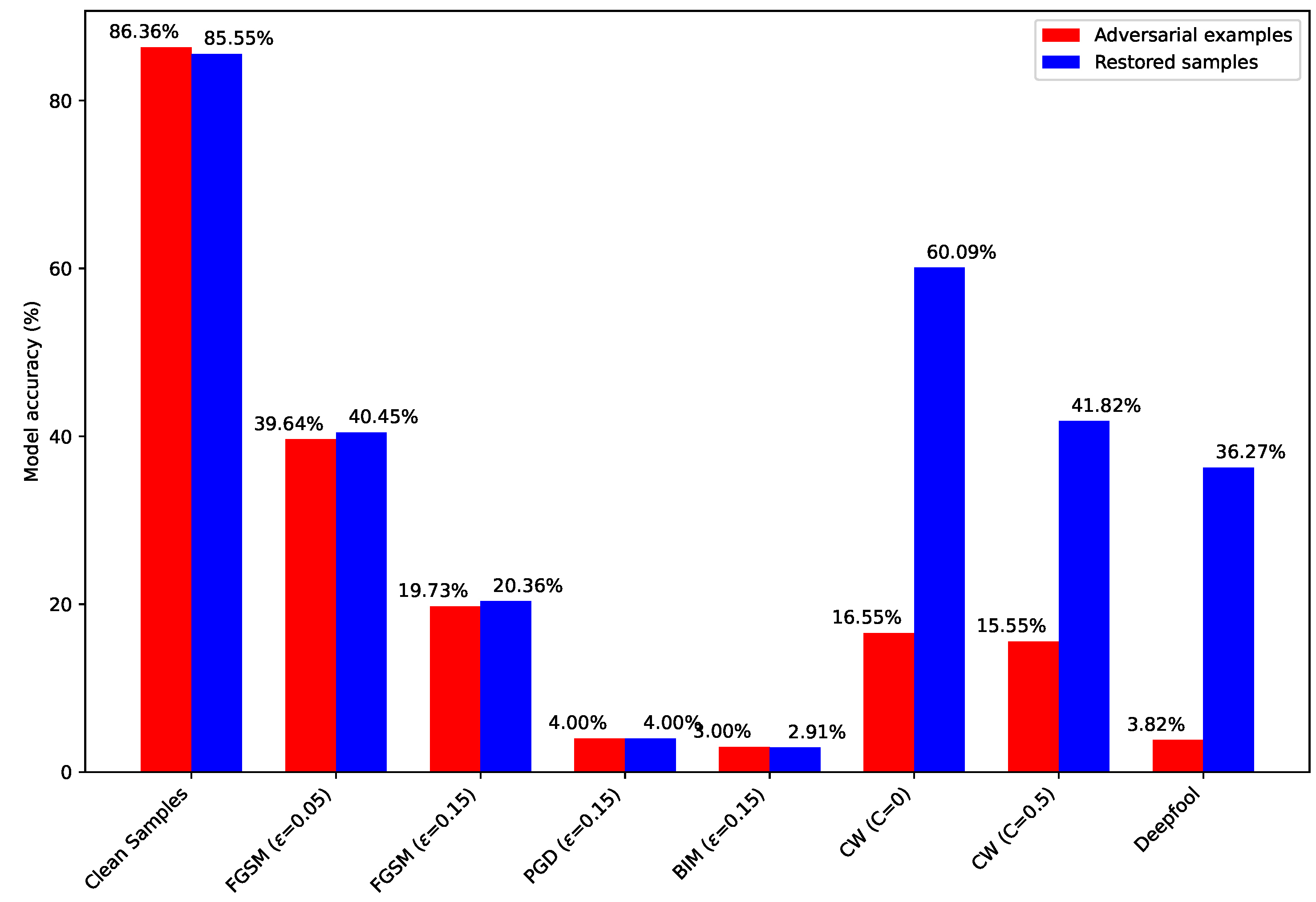
- All proposed frameworks and techniques were rigorously validated on the RML2016.10a dataset. Achieving a comprehensive detection rate of up to 88% for five classical adversarial examples, the model’s recognition rate improved by over 40% after the recovery of adversarial examples. These results compellingly attest to the effectiveness of the introduced framework.
2. Related Work
3. Description of Research Methods
3.1. Automatic Modulation Recognition
3.2. Adversarial Examples
3.2.1. Threat Model
3.2.2. Adversarial Attacks
Gradient-Based Attacks
Optimization-Based Attacks
3.3. Reconstruction Error
3.4. Kullback–Leibler Divergence
3.5. Adversarial Example Restoration
4. The Proposed Detection and Restoration Framework
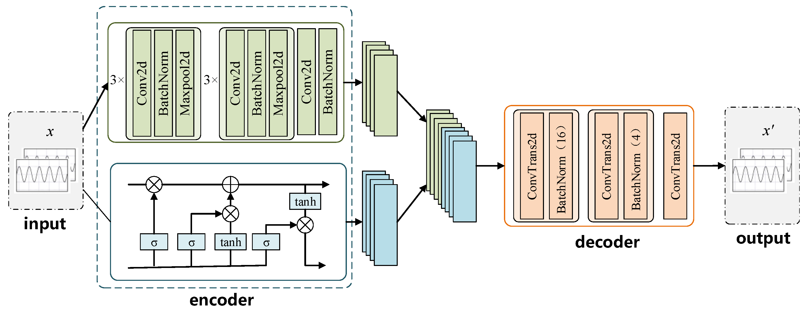
4.1. Detector Design
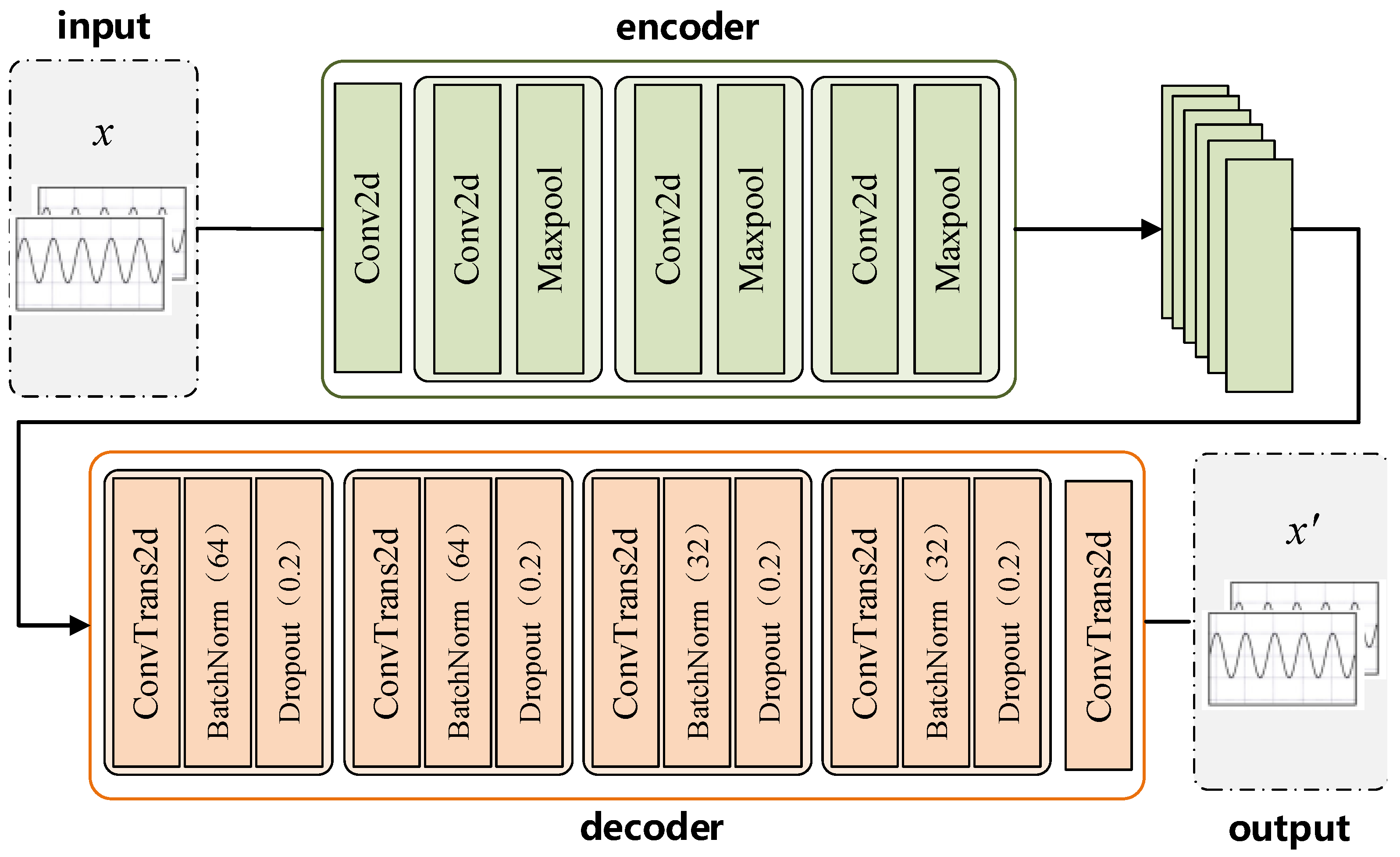
4.2. Restorer Design
4.3. Detection Method Based on Reconstruction Error
- Encoder: Produces a compressed data representation.
- Decoder: Reconstructs the original data from this representation.
| Algorithm 1: Reconstruction error-based adversarial detection. |
 |
4.4. Detection Method Based on KL Divergence
| Algorithm 2: Detection method based on kl divergence with classifier integration. |
 |
4.5. Adversarial Example Restorer Method
| Algorithm 3: Adversarial example restoration. |
|
5. Results and Discussion
5.1. Datasets
5.2. Classifier Model
5.3. Comparative Experiments on the Degree of Difference in Reconstruction Errors under Different Paradigms
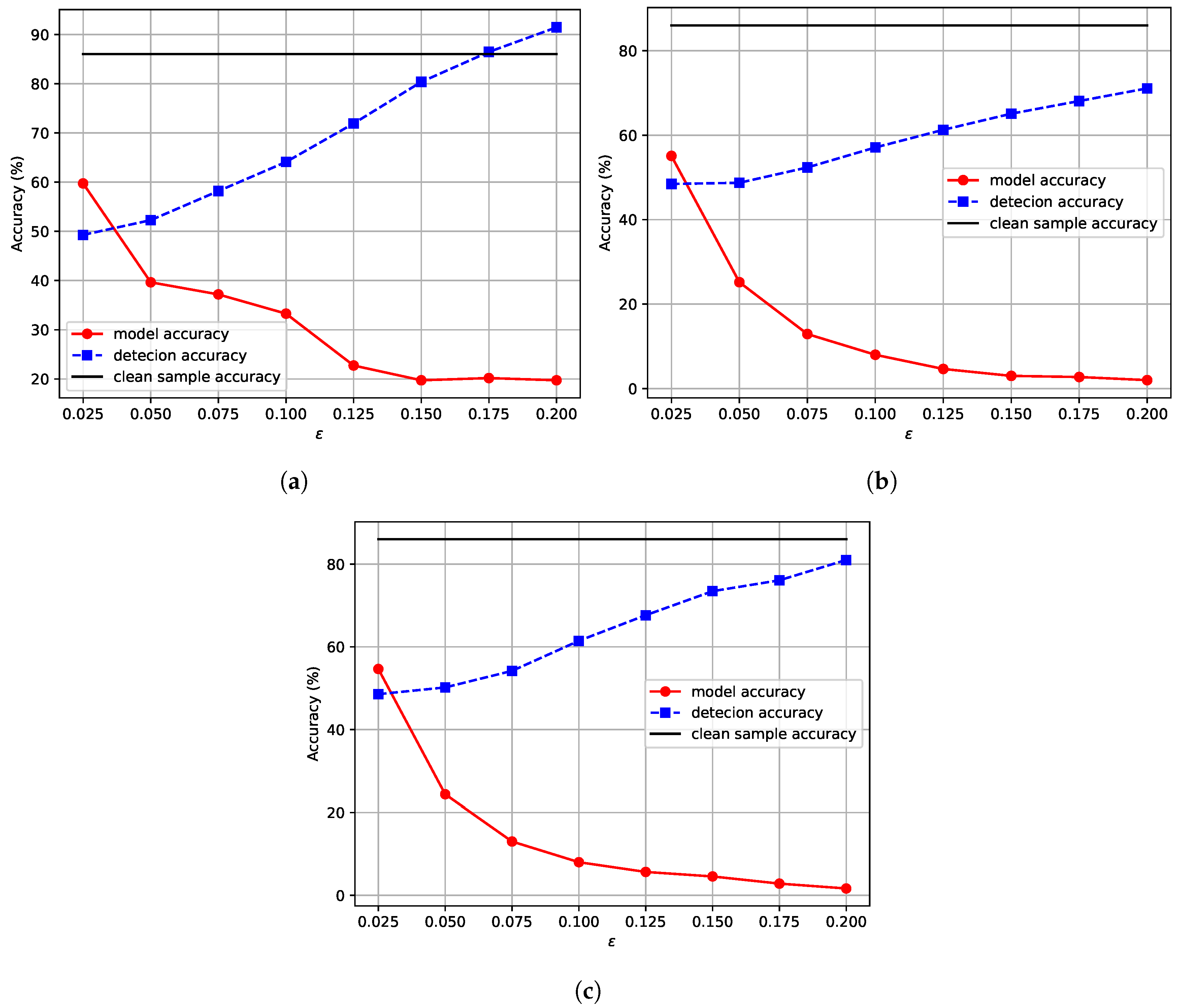
5.4. Detection Experiments for Various Attacks Based on Reconstruction Error
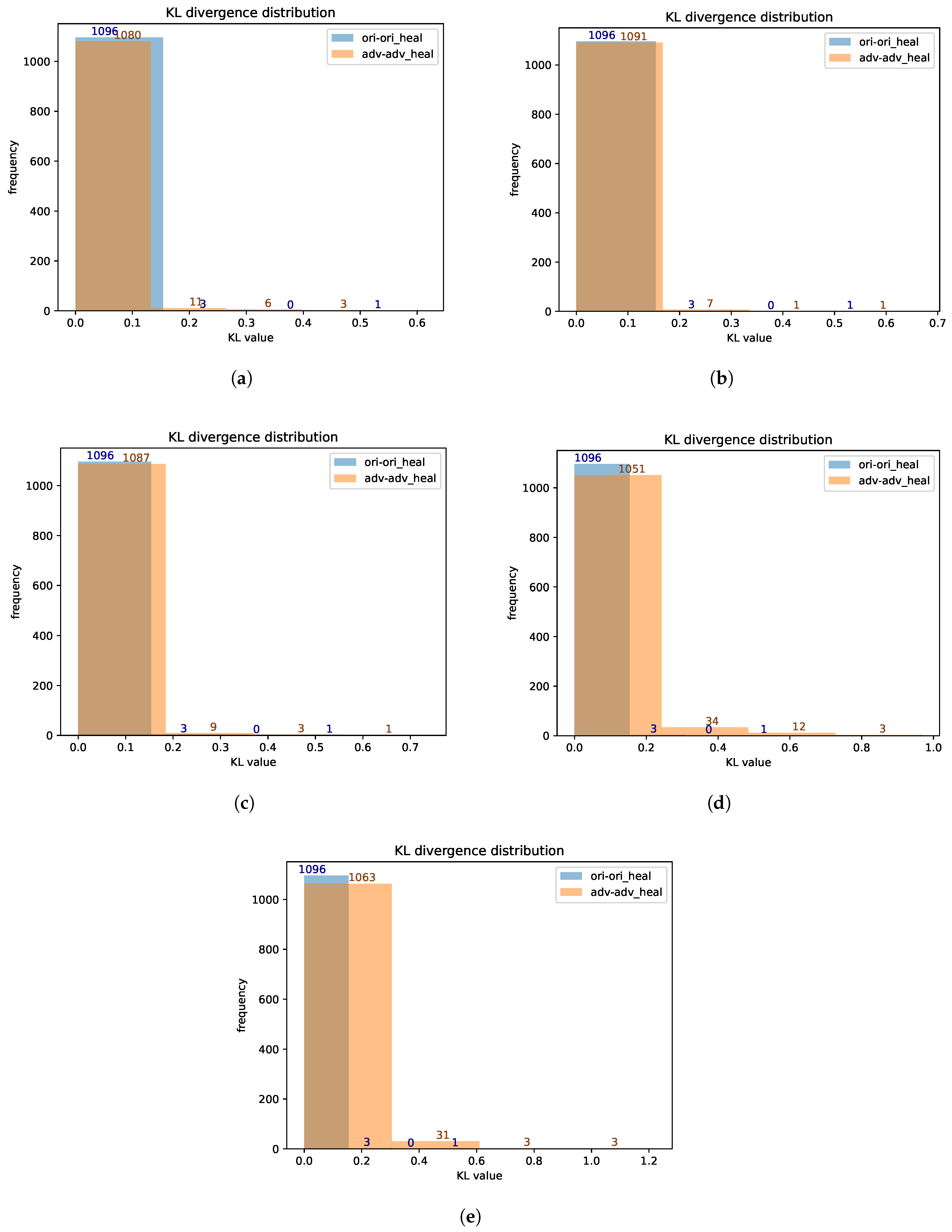
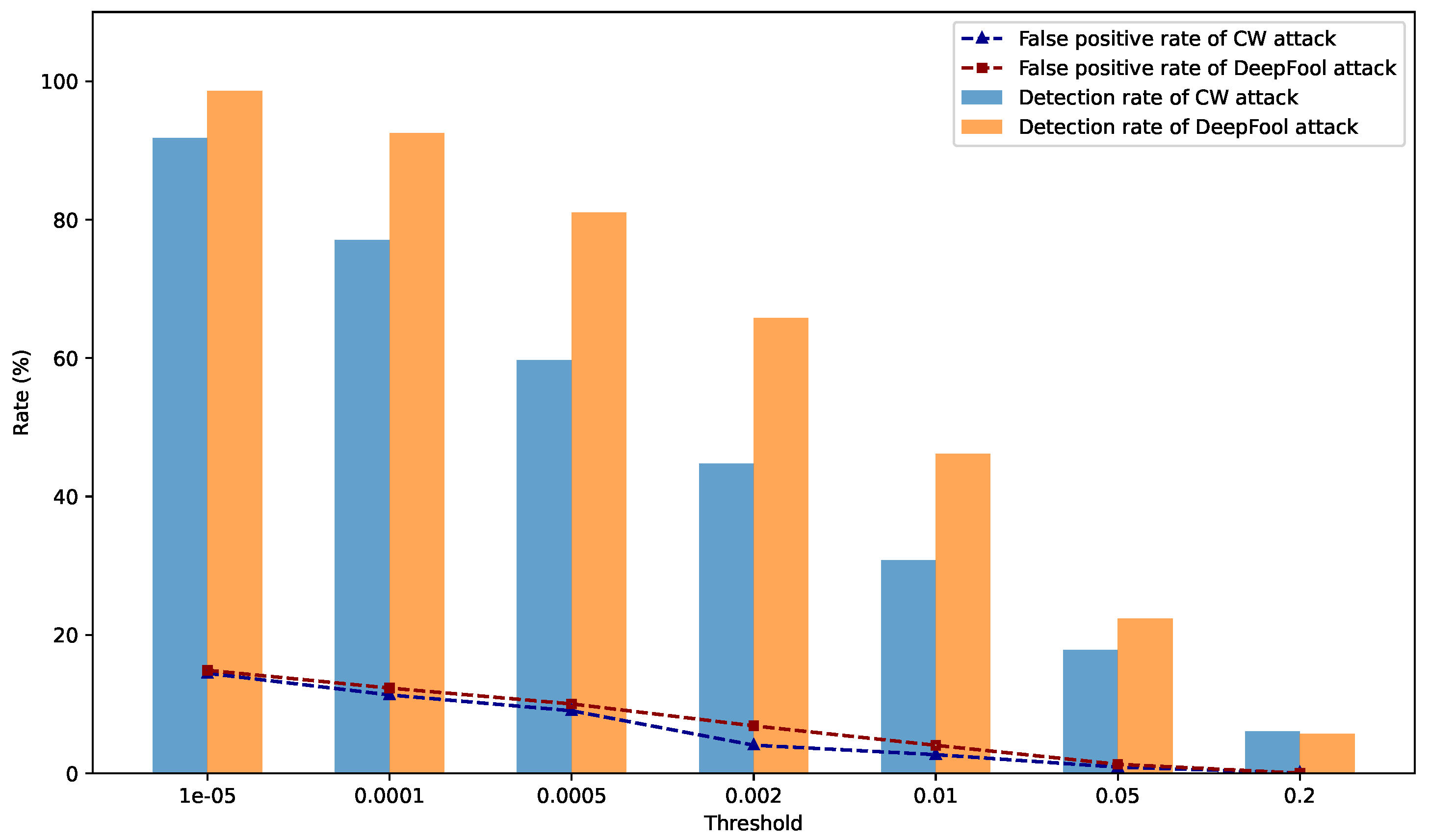
5.5. Detection Experiments for Various Attacks Based on KL Divergence
5.6. Comprehensive Detection Capability
5.7. Sample Restoration Experiment Based on Autoencoder
6. Conclusions
Author Contributions
Funding
Institutional Review Board Statement
Informed Consent Statement
Data Availability Statement
Conflicts of Interest
References
- Lin, Y.; Zha, H.; Tu, Y.; Zhang, S.; Yan, W.; Xu, C. GLR-SEI: Green and Low Resource Specific Emitter Identification Based on Complex Networks and Fisher Pruning. IEEE Trans. Emerg. Top. Comput. Intell. 2023, 1–12. [Google Scholar] [CrossRef]
- Zha, H.; Wang, H.; Feng, Z.; Xiang, Z.; Yan, W.; He, Y.; Lin, Y. LT-SEI: Long-Tailed Specific Emitter Identification Based on Decoupled Representation Learning in Low-Resource Scenarios. IEEE Trans. Intell. Transp. Syst. 2023, 1–15. [Google Scholar] [CrossRef]
- Lin, Y.; Tu, Y.; Dou, Z.; Chen, L.; Mao, S. Contour Stella Image and Deep Learning for Signal Recognition in the Physical Layer. IEEE Trans. Cogn. Commun. Netw. 2021, 7, 34–46. [Google Scholar] [CrossRef]
- Ya, T.; Yun, L.; Haoran, Z.; Zhang, J.; Yu, W.; Guan, G.; Shiwen, M. Large-scale real-world radio signal recognition with deep learning. Chin. J. Aeronaut. 2022, 35, 35–48. [Google Scholar]
- O’Shea, T.J.; Corgan, J.; Clancy, T.C. Convolutional radio modulation recognition networks. In Engineering Applications of Neural Networks: 17th International Conference, EANN 2016, Aberdeen, UK, 2–5 September 2016; Proceedings 17; Springer: Berlin/Heidelberg, Germany, 2016; pp. 213–226. [Google Scholar]
- Szegedy, C.; Zaremba, W.; Sutskever, I.; Bruna, J.; Erhan, D.; Goodfellow, I.; Fergus, R. Intriguing properties of neural networks. arXiv 2013, arXiv:1312.6199. [Google Scholar]
- Barreno, M.; Nelson, B.; Joseph, A.D.; Tygar, J.D. The security of machine learning. Mach. Learn. 2010, 81, 121–148. [Google Scholar] [CrossRef]
- Dalvi, N.; Domingos, P.; Mausam; Sanghai, S.; Verma, D. Adversarial classification. In Proceedings of the Tenth ACM SIGKDD International Conference on Knowledge Discovery and Data Mining, Seattle, WA, USA, 22–25 August 2004; pp. 99–108. [Google Scholar]
- Volchikhin, V.; Urnev, I.; Malygin, A.; Ivanov, A. Information-telecommunication system with multibiometric protection of user’s personal data. In Proceedings of the Progress in Electromagnetics Research Symposium, Moscow, Russia, 19–23 August 2012; pp. 71–74. [Google Scholar]
- Gu, T.; Dolan-Gavitt, B.; Garg, S. Badnets: Identifying vulnerabilities in the machine learning model supply chain. arXiv 2017, arXiv:1708.06733. [Google Scholar]
- Goodfellow, I.J.; Shlens, J.; Szegedy, C. Explaining and harnessing adversarial examples. arXiv 2014, arXiv:1412.6572. [Google Scholar]
- Madry, A.; Makelov, A.; Schmidt, L.; Tsipras, D.; Vladu, A. Towards Deep Learning Models Resistant to Adversarial Attacks. In Proceedings of the International Conference on Learning Representations, Vancouver, BC, Canada, 30 April–3 May 2018. [Google Scholar]
- Guo, C.; Rana, M.; Cisse, M.; Van Der Maaten, L. Countering adversarial images using input transformations. arXiv 2017, arXiv:1711.00117. [Google Scholar]
- Papernot, N.; McDaniel, P.; Wu, X.; Jha, S.; Swami, A. Distillation as a defense to adversarial perturbations against deep neural networks. In Proceedings of the 2016 IEEE Symposium on Security and Privacy (SP), San Jose, CA, USA, 22–26 May 2016; IEEE: Piscataway, NJ, USA, 2016; pp. 582–597. [Google Scholar]
- Samangouei, P.; Kabkab, M.; Chellappa, R. Defense-Gan: Protecting classifiers against adversarial attacks using generative models. In Proceedings of the 6th International Conference on Learning Representations, ICLR 2018, Vancouver, BC, Canada, 30 April–3 May 2018. [Google Scholar]
- Ponti, M.; Kittler, J.; Riva, M.; de Campos, T.; Zor, C. A decision cognizant Kullback–Leibler divergence. Pattern Recognit. 2017, 61, 470–478. [Google Scholar] [CrossRef]
- Youssef, A.; Delpha, C.; Diallo, D. An optimal fault detection threshold for early detection using Kullback–Leibler divergence for unknown distribution data. Signal Process. 2016, 120, 266–279. [Google Scholar] [CrossRef]
- Sadeghi, M.; Larsson, E.G. Adversarial attacks on deep-learning based radio signal classification. IEEE Wirel. Commun. Lett. 2018, 8, 213–216. [Google Scholar] [CrossRef]
- Sagduyu, Y.E.; Shi, Y.; Erpek, T. IoT network security from the perspective of adversarial deep learning. In Proceedings of the 2019 16th Annual IEEE International Conference on Sensing, Communication, and Networking (SECON), Boston, MA, USA, 10–13 June 2019; IEEE: Piscataway, NJ, USA, 2019; pp. 1–9. [Google Scholar]
- Bair, S.; DelVecchio, M.; Flowers, B.; Michaels, A.J.; Headley, W.C. On the limitations of targeted adversarial evasion attacks against deep learning enabled modulation recognition. In Proceedings of the ACM Workshop on Wireless Security and Machine Learning, Miami, FL, USA, 15–17 May 2019; pp. 25–30. [Google Scholar]
- Kokalj-Filipovic, S.; Miller, R.; Morman, J. Targeted adversarial examples against RF deep classifiers. In Proceedings of the ACM Workshop on Wireless Security and Machine Learning, Miami, FL, USA, 15–17 May 2019; pp. 6–11. [Google Scholar]
- Kokalj-Filipovic, S.; Miller, R.; Vanhoy, G. Adversarial examples in RF deep learning: Detection and physical robustness. In Proceedings of the 2019 IEEE Global Conference on Signal and Information Processing (GlobalSIP), Ottawa, ON, Canada, 11–14 November 2019; IEEE: Piscataway, NJ, USA, 2019; pp. 1–5. [Google Scholar]
- Flowers, B.; Buehrer, R.M.; Headley, W.C. Evaluating adversarial evasion attacks in the context of wireless communications. IEEE Trans. Inf. Forensics Secur. 2019, 15, 1102–1113. [Google Scholar] [CrossRef]
- Lin, Y.; Zhao, H.; Ma, X.; Tu, Y.; Wang, M. Adversarial attacks in modulation recognition with convolutional neural networks. IEEE Trans. Reliab. 2020, 70, 389–401. [Google Scholar] [CrossRef]
- Bao, Z.; Lin, Y.; Zhang, S.; Li, Z.; Mao, S. Threat of adversarial attacks on DL-based IoT device identification. IEEE Internet Things J. 2021, 9, 9012–9024. [Google Scholar] [CrossRef]
- Ren, K.; Zheng, T.; Qin, Z.; Liu, X. Adversarial attacks and defenses in deep learning. Engineering 2020, 6, 346–360. [Google Scholar] [CrossRef]
- Tian, Q.; Zhang, S.; Mao, S.; Lin, Y. Adversarial attacks and defenses for digital communication signals identification. Digit. Commun. Netw. 2022. [Google Scholar] [CrossRef]
- Kim, B.; Sagduyu, Y.E.; Davaslioglu, K.; Erpek, T.; Ulukus, S. Channel-aware adversarial attacks against deep learning-based wireless signal classifiers. IEEE Trans. Wirel. Commun. 2021, 21, 3868–3880. [Google Scholar] [CrossRef]
- Wójcik, B.; Morawiecki, P.; Śmieja, M.; Krzyżek, T.; Spurek, P.; Tabor, J. Adversarial Examples Detection and Analysis with Layer-wise Autoencoders. In Proceedings of the 2021 IEEE 33rd International Conference on Tools with Artificial Intelligence (ICTAI), Washington, DC, USA, 1–3 November 2021; pp. 1322–1326. [Google Scholar] [CrossRef]
- Li, T.; Luo, W.; Shen, L.; Zhang, P.; Ju, X.; Yu, T.; Yang, W. Adversarial sample detection framework based on autoencoder. In Proceedings of the 2020 International Conference on Big Data & Artificial Intelligence & Software Engineering (ICBASE), Bangkok, Thailand, 30 October–1 November 2020; pp. 241–245. [Google Scholar] [CrossRef]
- Ye, H.; Liu, X. Feature autoencoder for detecting adversarial examples. Int. J. Intell. Syst. 2022, 37, 7459–7477. [Google Scholar] [CrossRef]
- Xiao, Y.; Pun, C.M. Improving adversarial attacks on deep neural networks via constricted gradient-based perturbations. Inf. Sci. 2021, 571, 104–132. [Google Scholar] [CrossRef]
- Kurakin, A.; Goodfellow, I.; Bengio, S. Adversarial machine learning at scale. arXiv 2016, arXiv:1611.01236. [Google Scholar]
- Carlini, N.; Wagner, D. Towards evaluating the robustness of neural networks. In Proceedings of the 2017 IEEE Symposium on Security and Privacy (SP), San Jose, CA, USA, 22–24 May 2017; IEEE: Piscataway, NJ, USA, 2017; pp. 39–57. [Google Scholar]
- Moosavi-Dezfooli, S.M.; Fawzi, A.; Frossard, P. Deepfool: A simple and accurate method to fool deep neural networks. In Proceedings of the IEEE Conference on Computer Vision and Pattern Recognition, Las Vegas, NV, USA, 27–30 June 2016; pp. 2574–2582. [Google Scholar]


| Norm | Original Sample | FGSM ( = 0.15) | BIM ( = 0.15) | PGD ( = 0.15) | CW | Deepfool |
|---|---|---|---|---|---|---|
| 0.9999 | 1.0 | 1.0 | 1.0 | 1.0 | 1.0 | |
| 0.0387 | 0.0264 | 0.0327 | 0.0311 | 0.0387 | 0.0380 | |
| 0.0021 | 0.0012 | 0.0016 | 0.0015 | 0.0022 | 0.0021 | |
| 0.0530 | 0.0370 | 0.0449 | 0.0430 | 0.0530 | 0.0520 |
| Sample Type | 0.0005 | 0.0006 | 0.0007 | 0.0008 | 0.0009 | 0.001 | 0.002 | 0.005 | 0.01 |
|---|---|---|---|---|---|---|---|---|---|
| Original | 0.7064 | 0.3845 | 0.2918 | 0.1773 | 0.1082 | 0.0727 | 0.0009 | 0.0 | 0.0 |
| FGSM | 0.9036 | 0.8036 | 0.6609 | 0.5573 | 0.4373 | 0.3445 | 0.0109 | 0.0 | 0.0 |
| PGD | 0.8500 | 0.7300 | 0.5836 | 0.4409 | 0.3155 | 0.2191 | 0.0018 | 0.0 | 0.0 |
| CW | 0.6873 | 0.4709 | 0.2873 | 0.1727 | 0.1055 | 0.0699 | 0.0018 | 0.0 | 0.0 |
| Attack Types | Detection Rate | Parameters | Detection Method | Threshold |
|---|---|---|---|---|
| FGSM | 91.45% | = 0.2 | reconstruction error | 0.0006 |
| PGD | 81% | = 0.2 | reconstruction error | 0.0006 |
| BIM | 71% | = 0.2 | reconstruction error | 0.0006 |
| CW | 99.09% | confidence = 0 | KL divergence | 0.0002 |
| Deepfool | 99.90% | overshoot = 0.005 | KL divergence | 0.0002 |
| overall detection rate | 88.488% | |||
Disclaimer/Publisher’s Note: The statements, opinions and data contained in all publications are solely those of the individual author(s) and contributor(s) and not of MDPI and/or the editor(s). MDPI and/or the editor(s) disclaim responsibility for any injury to people or property resulting from any ideas, methods, instructions or products referred to in the content. |
© 2023 by the authors. Licensee MDPI, Basel, Switzerland. This article is an open access article distributed under the terms and conditions of the Creative Commons Attribution (CC BY) license (https://creativecommons.org/licenses/by/4.0/).
Share and Cite
Han, C.; Qin, R.; Wang, L.; Cui, W.; Li, D.; Yan, B. Adversarial Example Detection and Restoration Defensive Framework for Signal Intelligent Recognition Networks. Appl. Sci. 2023, 13, 11880. https://doi.org/10.3390/app132111880
Han C, Qin R, Wang L, Cui W, Li D, Yan B. Adversarial Example Detection and Restoration Defensive Framework for Signal Intelligent Recognition Networks. Applied Sciences. 2023; 13(21):11880. https://doi.org/10.3390/app132111880
Chicago/Turabian StyleHan, Chao, Ruoxi Qin, Linyuan Wang, Weijia Cui, Dongyang Li, and Bin Yan. 2023. "Adversarial Example Detection and Restoration Defensive Framework for Signal Intelligent Recognition Networks" Applied Sciences 13, no. 21: 11880. https://doi.org/10.3390/app132111880