SSCL-TransMD: Semi-Supervised Continual Learning Transformer for Malicious Software Detection

Abstract

Machine learning-based malware (malicious software) detection methods have a wide range of real-world applications. However, these types of approaches suffer from the fatal problem of “model aging”, in which the validity of the model decreases rapidly as the malware continues to evolve and variants emerge continuously. The model aging problem is usually solved by model retraining, which relies on lots of labeled samples obtained at great expense. To address this challenge, this paper proposes a semi-supervised continuous learning malware detection model based on Transformer. Firstly, this model improves the lifelong semi-supervised mixture algorithm to dynamically adjust the weighted combination of new sample sequences and historical ones to solve the imbalance problem. Secondly, the Learning with Local and Global Consistency algorithm is used to iteratively compute similarity scores for the unlabeled samples in the mixed samples to obtain pseudo-labels. Lastly, the Multilayer Perceptron is applied for malware classification. To validate the effectiveness of the model, this paper conducts experiments on the CICMalDroid2020 dataset. The experimental results show that the proposed model performs better than existing deep learning detection models. The F1 score has an average improvement of 1.27% compared to other models when conducting binary classification. And, after inputting hybrid samples, including historical data and new data, four times, the F1 score is still 1.96% higher than other models.

1. Introduction

In recent years, with the rapid development of digitization and the increasing convenience of internet technology, mobile devices such as smartphones have rapidly evolved. The Android system, due to its open source nature, has gradually become the mobile operating system with the highest market share. However, this also makes it the primary target for malicious software developers, which brings great harm to individual and enterprise data users. According to the “2020 Android Platform Security Situation Analysis Report” by Qi An Xin Threat Intelligence Center, a total of 2.3 million malicious Android program samples were intercepted in 2020, with an average of 6301 malicious program samples intercepted per day. According to the “China Mobile Security Situation Report for the First Half of 2022” released by 360 Anti-Phishing Center, approximately 10.797 million mobile malicious program samples were intercepted in the first half of 2022, a year-on-year increase of 180.5% compared to the first half of 2021.

The rapid spread of malicious software has brought about a large number of harms, such as fee consumption, privacy leakage, and remote control, all of which mobile smartphone users have to bear. According to the “2020 Android Platform Security Situation Analysis Report”, security governance of mobile internet is relatively weak globally and presents various means, such as online banking theft and Trojan problems, which pose a great threat to users’ property. Unlike other operating systems, the Android operating system allows users to obtain applications from third-party app stores, which brings convenience to users but also risks and hazards. The presence of unverified applications in third-party app stores increases the likelihood of users downloading malicious software.

Although there have been continuous developments in technologies for malware detection, and significant progress has been made, malware developers are also utilizing the latest technologies to update their malicious software. Different categories of malware, such as Trojans, adware, and riskware, are constantly being developed. Therefore, efficient malware detection methods are essential.

Deep learning, as a powerful tool for data pattern mining, has been widely applied in the field of malware detection. In the training of malware detection models, static datasets collected in advance are usually used for learning. This results in the inability of the models to detect unknown malicious behaviors. Therefore, predicting unknown malicious behaviors based on historical samples of malicious behaviors is a challenging task, and the ability to continuously learn new unlabeled malicious software behavior information is crucial for the lifespan of a malware detection system.

In recent years, the Transformer model, known for its high degree of parallelism and scalability in parallel computing systems, has become a star in the field of deep learning. Many improved Transformer models have achieved excellent results in malware detection. Although these improved Transformer models have clear advantages, there are two pressing issues that need to be addressed for application in the field of malware detection: (1) Due to the continuous updates of malware data, the obtained samples of malicious software lack labels, which poses great difficulties in training malware detection models; (2) The fixed structure of deep learning neural networks determines the limited capacity of the models [1]. When neural networks learn new malicious software behaviors, they may forget historical data, leading to catastrophic forgetting [2]. To address catastrophic forgetting, one approach is to incorporate new samples into the historical training dataset and retrain the network using a dataset that contains both new and old training data. However, starting from scratch to train the model to adapt to newly generated malicious software data every day is time-consuming and highly inefficient.

This paper makes the following contributions:

1.

It proposes a semi-supervised SSCL-TransMD malware detection model. The proposed model improves a feature memory replay algorithm and a pseudo-labels acquisition algorithm;

2.

It apples the memory buffer to improve the existing method to solve the significant imbalance between the new samples and historical samples caused by the the fixed weighted combination of new sample sequences and historical ones;

3.

The proposed model is validated on CICMalDroid2020 datasets. The experimental results demonstrate that the SSCL–TransMD model outperforms other detection models in malware detection tasks.

2. Related Work

Malware detection methods can be broadly classified into three categories: traditional malware detection methods, machine learning-based malware detection methods, and deep learning-based malware detection methods. In the following Sections, each of these methods are discussed in detail.

Traditional malware detection methods primarily rely on feature-based matching using unique features extracted from APK files within software [3]. These methods match the extracted features against a database of known malware features to determine whether the target software is malicious. If a match is found, the target software is classified as malware; otherwise, it is considered benign. One key limitation of this method is its dependency on a database of known malware features. As a result, it is easily affected when attackers use obfuscation techniques to alter the syntax of the software and modify the feature codes. While this method can detect malware through precise matching with known feature codes, it is unable to handle unknown malware [4].

Machine learning-based malware detection operates by first extracting various behavioral features from the sample under analysis [5]. These features are then represented as fixed-dimensional vectors. Finally, existing machine learning algorithms are used to train the classifier on labeled samples, enabling the prediction of the class for unknown samples.

Faiz, Hussain, and Marchang [6] utilized features extracted from permissions, broadcast receivers, and APIs to apply support vector machine for detecting Android malware, achieving a classification accuracy of 98.55%. Alqahtani, Zagrouba, and Almuhaideb [7] reviewed machine learning detectors and provided a detailed summary of the applications of naive Bayes, support vector machine, and deep neural networks in Android malware detection. Lashkari et al. [8] compared random forest, K-nearest neighbor, and decision tree algorithms as classifiers for Android malware detection, employing the same selected features for training, testing, and evaluation in each machine learning algorithm. The K-nearest neighbor algorithm [9] operates as a supervised learning model that achieves the classification of Android malware by measuring the Euclidean distance between different feature values in the geometric space. K-means clustering algorithm [10], an unsupervised learning algorithm, is typically employed for family categorization of Android malware with the objective of finding centroids among N data points, thereby minimizing the mean square distance from each data point to its nearest centroid. Zhao et al. [11] aimed to improve the accuracy of Android malware detection by employing boosting and bagging. Rana and Sung [12] achieved improved accuracy in Android malware detection by combining multiple machine learning classifiers within ensemble learning. Yerima and Sezer [13] proposed a novel multi-level structured classifier fusion approach, training lower-level Android base classifiers to generate models and using a ranking algorithm to select the final classifier, then assigning weights to the prediction results of the selected classifier based on the prediction accuracy of higher-level base classifiers. However, due to the requirement for multiple detectors to analyze each APK file, the application of ensemble learning is computationally expensive. Birman et al. [14] addressed this issue by employing deep reinforcement learning to automatically start and stop basic classifiers, dynamically determining whether sufficient information is available to classify a given APK file using a deep neural network.

Deep learning is a machine learning method based on representation learning of data [15]. Deep learning techniques can integrate feature learning into the learning process of models, thereby reducing the defects caused by manually training features.

The DL-Droid framework [16] proposes a new method for detecting Android malware using dynamic analysis techniques based on deep learning technology. In the case of considering only dynamic features, the detection rate of this method is 97.8%. When static features are added, the detection rate increases to 99.6%. In addition, the DL-Droid framework [16] compares detection performance and code coverage, and compares the performance of traditional machine learning classifiers, showing that this method outperforms machine learning-based methods. Vinayakumar et al. [17] proposed a hybrid malware classification method using segmentation-based fractal texture analysis and deep convolutional neural network features. Android APKs are binarized into grayscale images generated using bytecode information. Vinayakumar et al. [17] used the time-reversal backpropagation algorithm to train long short-term memory neural networks for detecting Android malware. Two different network topologies are used: a standard long short-term memory neural network with only one hidden layer and a stacked long short-term memory neural network with three hidden layers. High detection accuracy for Android malware is demonstrated in both static and dynamic analysis. DeepRefiner [18] uses long short-term memory neural networks to perform two-layer detection and verification of the semantic structure of Android bytecode. The accuracy of this method is 97.4%, with a false positive rate of 2.54%. Compared to traditional methods, this method has higher efficiency and accuracy. M. Amin et al. [19] extracted vectorized opcodes from APKs’ bytecode using one-hot encoding to detect malware attributes. By performing experiments with recurrent neural networks, long short-term memory networks, neural networks, deep convolutional networks, and sparse autoencoder models, bi-directional long short-term memory neural networks were found to be the best model for this method. The AdMat [20] model uses a matrix-based convolutional neural network approach for detecting Android malware. This approach treats applications as features and views them as images. An adjacency matrix of the application has been constructed to improve data processing efficiency. This paper used convolutional neural network methods to analyze API sequence calls, opcodes, and permissions for the detection of Android malware in Zero-Day scenarios.

Oak et al. [21] used deep learning techniques to detect Android malware based on dynamic analysis of application activity sequences. The paper showed that analyzing a series of activities can provide information for detecting malware, but analyzing longer sequences does not necessarily result in more accurate models. In the real world, the number of malware instances is smaller than the number of harmless applications. The dataset in the paper contains over 180,000 samples, with two-thirds being malware. This dataset is significantly larger than other datasets used in previous research. The paper simulates real-world situations by randomly sampling a small portion of malware samples. Using the state-of-the-art BERT (Bidirectional Encoder Representations from Transformers) model, the paper demonstrates ideal malware detection performance in an extremely unbalanced dataset. Experimental results verify the effectiveness of this method in handling highly imbalanced datasets.

3. Methodology

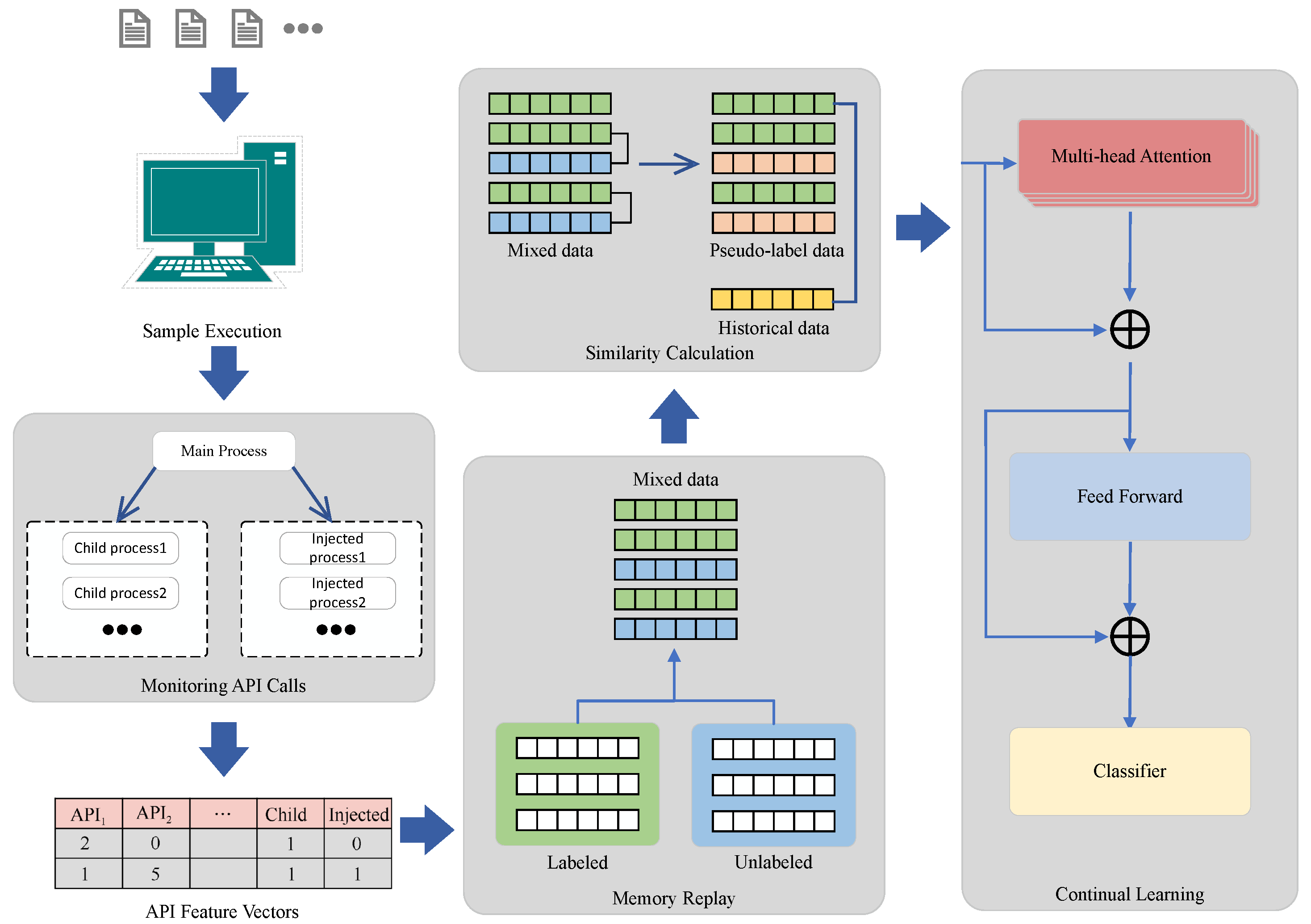
The SSCL–TransMD detection model is mainly composed of five layers, namely, the memory replay layer, information mapping layer, similarity calculation layer, information encoding layer, and classification detection layer. Each layer is responsible for receiving the input of weighted historical sample sequences and new sample sequences, mapping the input sequence, providing pseudo-labels for the input sequence, feature encoding, as well as training the model and outputting the final classification results.

In the SSCL–TransMD detection model, the input data consist of data sequences generated during the operation of different categories of malware, and the output data are the identification result of malware. The overall structure of the SSCL–TransMD detection model is shown in Figure 1.

The following Sections provide a detailed introduction to the model structure:

Memory Replay Layer: The inputs of this layer are the malware data after static analysis. The required sub-sample B for each learning iteration is divided in advance. At the first layer, they are sequence data $A_1$. At the i-th layer, the data from $A_1$ to $A_i$ layers are combined through the memory replay sampling method and given to the information mapping layer;

Similarity Calculation Layer: The input of this layer is the feature matrix generated by the information mapping layer. The feature matrix is composed of countless vectors. The LLGC algorithm is iteratively used in the similarity calculation layer to calculate the similarity matrix between labeled vectors and unlabeled vectors, thus obtaining similarity scores. The similarity scores are used as input for the unlabeled vectors, and the feature matrix obtained from the information mapping layer in the information coding layer;

Information Mapping Layer: The inputs of this layer are the sequence data $A_i$ obtained from the memory replay layer. After preprocessing the sequence data $A_i$, the malware data size and annotation format are adapted to the model. During each training iteration, a sub-sample $A_i$ is obtained from the dataset, and the input data size is A × L × W, where L represents the number of malware features in the input and W represents the dimension of the data after mapping by the input layer;

Information Coding Layer: The input of this layer is the feature matrix generated by the similarity calculation layer and its corresponding similarity labels. The information coding layer consists of three layers: multi-head attention mechanism layer, residual connection and normalization layer, and fully connected layer. The feature matrix is learned using multi-head attention, then passed through the residual connection and normalization layer to perform residual connection on the sequence matrix weighted by the feature, followed by a linear transformation to map the data, which are finally mapped by the fully connected layer to learn more abstract features;

Classification Detection Layer: The input of this layer is the matrix obtained from the information coding layer. The classification detection layer consists of an MLP basic neural network, which adjusts the matrix dimension provided by the information coding layer through the MLP fully connected layer, then performs classification and outputs the classification results through the softmax activation function. The specific model and parameters are detailed in the next chapter. After training, the model parameters converge to achieve optimal prediction performance. The test dataset is input into the trained model to output the recognition results of the test dataset.

3.1. Model Components

The SSCL–TransMD detection model proposed in this chapter mainly consists of three key components, namely, the memory replay component, the similarity calculation component, and the classification detection component. The SSCL–TransMD detection model uses an improved LUMP model as the memory replay component, selects the LLGC label iteration algorithm as the similarity calculation component, analyzes the characteristics of malicious software sequences, and selects the MLP basic neural network as the classification detection component. This Section provides a detailed introduction to the three components used in the SSCL-TransMD detection model.

3.1.1. Memory Replay Component

The memory replay component is one of the core components of semi-supervised continual learning. The purpose of this component is to mix historical labeled malicious software sample sequences and unlabeled new malicious software sample sequences according to the principles of continual learning [22], using certain weights. This subsection discusses how the principles of continual learning are applied in the field of malicious software and how the memory replay method for malicious software samples is utilized in this chapter.

(1)

Continuous Learning

When the malware detection model transitions into batch learning mode, it is easy to forget the old malware classifications. This means that, after updating the model with new malware data, the classification performance achieved by the malware detection model in historical tasks will rapidly decline, leading to catastrophic forgetting. The root cause of catastrophic forgetting is that the training process for the new malware classification task requires changing the weights of the historical neural network. This inevitably modifies certain weights that are crucial for the historical malware detection task, rendering the malware detection model no longer suitable for historical tasks. 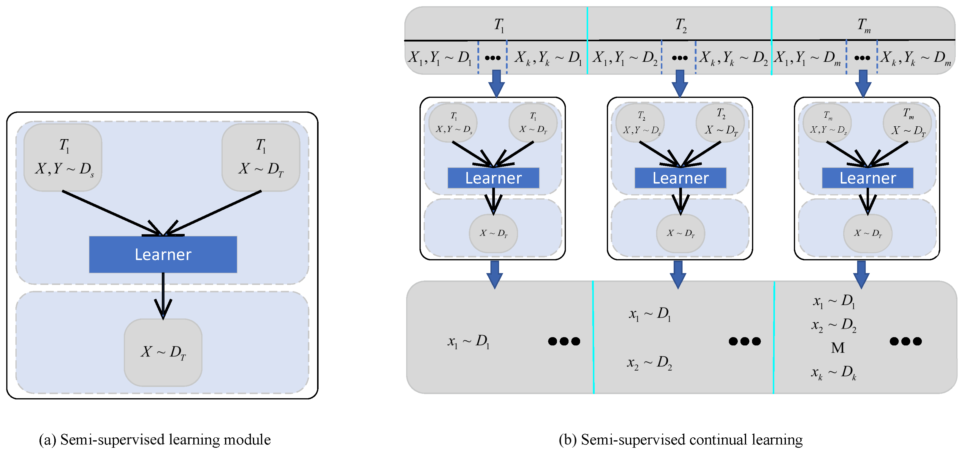To overcome catastrophic forgetting, the malware detection model needs to not only demonstrate the ability to acquire new knowledge in new classification tasks, but also prevent significant interference from new malware data on the existing model [23]. In this Section, we use a continuous learning approach to continuously train the malware detection model.

The process of continuous learning for a malware model, denoted as P, is shown in Equations (1) and (2):

$$P=\left\{P_1,P_2,\dots ,P_n,\dots \right\}$$

(1)

$$P_n:〈M_{n-1},T_n〉\to M_n$$

(2)

The initial malware detection model before continuous learning is represented as $M_0$, and the continuous input of newly added malware behavior data sequence is represented as $T=T_1,T_2,\dots ,T_n,\dots ,T_n=(X_n^i,Y_n^i)|i=1,2,\dots ,N_n$, where $X_n^i$ and $Y_n^i$ are the dataset instances and corresponding labels of the first i malware sequences at task $T_n$. The malware detection model after learning from $T_n$ is represented as $M_n$. The process of semi-supervised continual learning is shown in Figure 2.

(2)

Memory Replay Method

The LUMP model is able to sample between the current batch and the historical sequences of malicious software inputs, effectively mitigating the catastrophic forgetting problem. It is a lifelong unsupervised learning method.

The training idea of the LUMP model is to mixup two random samples $(x_i,y_i)$ and $(x_j,y_j)$ together with the weight $\lambda$ to form a new sample, as shown in Equation (3):

$$\left\{\begin{array}{c}\tilde{x}=\lambda ·x_i+\left(1-\lambda \right)·x_j\\ \tilde{y}=\lambda ·y_i+\left(1-\lambda \right)·y_j\end{array}\right.$$

(3)

The standard mixup [24] training contructs virtual training examples based on the principle of Vicinal Risk Minimization. Let $(x_i,y_i)$ and $(x_j,y_j)$ denote two random feature–target pairs sampled from the training data distribution, and let $(\overline{x},\overline{y})$ denote the interpolated feature–target pair in the vicinity of these examples; mixup then minimizes the following objective:

$$\begin{array}{cc}\hfill L_{mixup}(\overline{x},\overline{y})& =CE(h_{\psi }\left(f_{\ominus }\left(\overline{x}\right)\right),\overline{y}),\hfill \\ \hfill where\overline{x}& =\lambda x_i+(1-\lambda )x_{j}and\overline{y}=\lambda y_i+(1-\lambda )y_j\hfill \end{array}$$

(4)

where $f_{\ominus }$ is an encoder network which is composed of a backbone network and $h_{\psi }$ is prediction MLP head, $\lambda \sim Beta(\alpha ,\alpha )$, for $\alpha \in (0,\infty )$. LUMP utilzes mixup for UCL (unsupervised continuous learning) by incorporating the instances stored in the replay buffer from the previous task into the vicinal distribution. More specificly, LUMP interpolates between the examples of the current task $\left(x_{i,\tau }\right)\in U_{\tau }$ and random examples selected using uniform sampling from the replay buffer, which encourages the model to behave linearly across a sequence of tasks. For current task $\tau$, LUMP minimizes the objective on the following interpolated instances $x_{i,\tau }$:

$${\tilde{x}}_{i,\tau }=\lambda ·x_{i,\tau }+\left(1-\lambda \right)·x_{i,M}$$

(5)

where $x_{j,M}\sim M$ denotes the example selected using uniform sampling from replay buffer M. The interpolated example not only augments the past tasks’ instances in the replay buffer, but also approximates regularized loss minimization [24]. During unsupervised continuous learning, LUMP enhances the robustness of learned representation by revisiting the attributes of the past task that are similar to the current. As a result, LUMP sucessively mitigates catastrophic forgetting.

Although the LUMP model partially avoids the catastrophic forgetting problem, there still exists an issue regarding the proportion between historical sample sequences and new input malicious software sample sequences. In the LUMP model, the weight $\lambda$ for the historical sample sequence and the new input malicious software sample sequence is fixed, which introduces a new problem. As the number of continuous learning training increases, the number of historical sample sequences also increases. At this time, the imbalance between the new task data and the historical sample data causes a data imbalance problem [25].

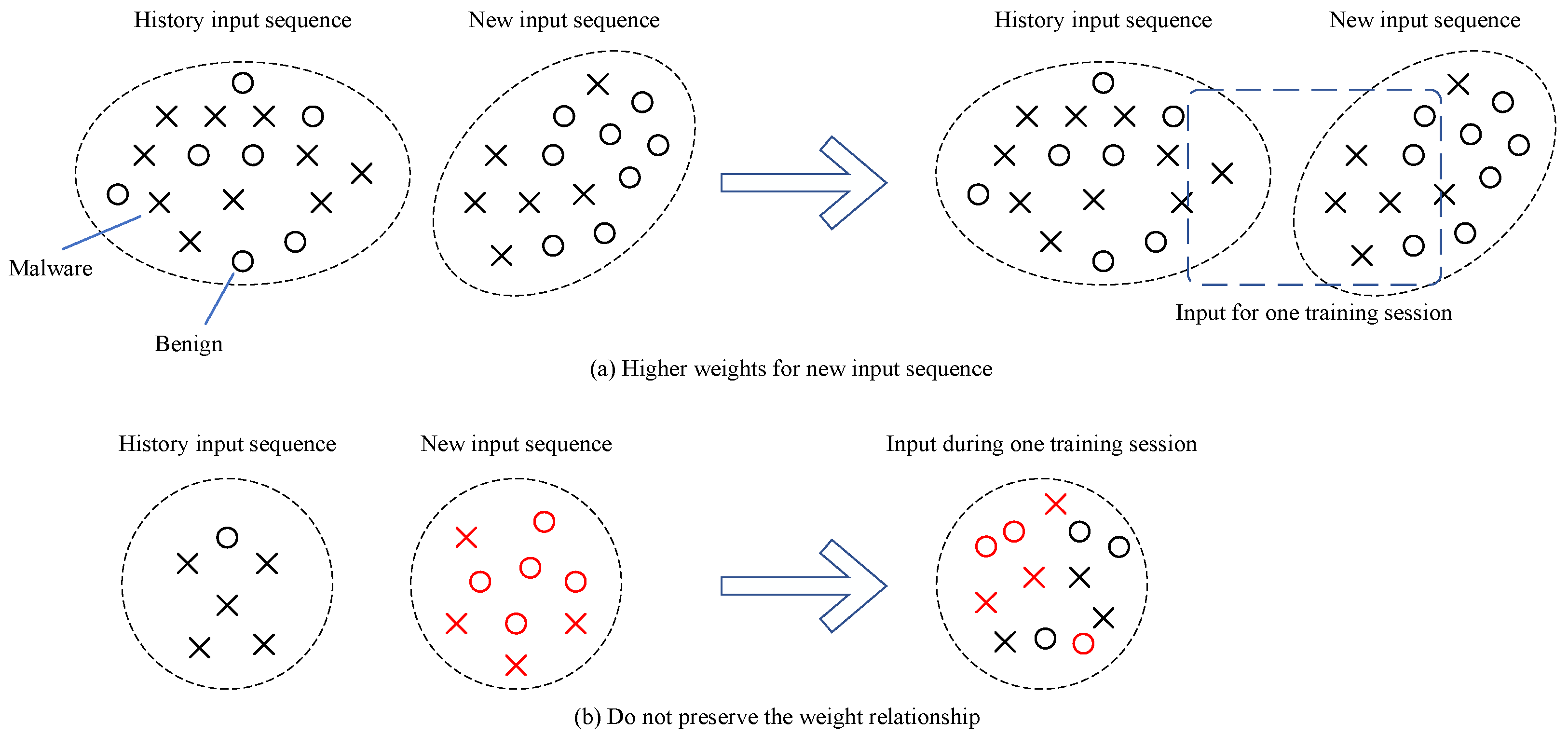
Specifically, in the training algorithm based on memory replay, only a few old class samples are seen, while there are more new class samples. In this case, the focus of the training process clearly shifts towards the new class, resulting in many detrimental effects on class-specific weights, as shown in Figure 3a, where the weights of new sequence data are significantly higher than those of old sequence data. From Figure 3b, it can be seen that the relationship between the labels of old data and their corresponding weights is not well preserved. The combination of these effects severely misleads the classifier, leading to decision biases towards confusion between new and old classes. These effects seriously cause the model to forget malicious behaviors in the old sequences during the analysis of malicious behavior.

To address these problems, this subsection proposes improvements to the training idea of the LUMP model in the memory replay component.

First, assume a memory replay buffer M that provides historical malicious software sample sequences. It mixes the historical input sequences stored in the memory replay buffer with new input malicious software detection samples. In other words, for the current input sequence $x_{i,\tau }\in T$ and the sequence sampled from the memory replay buffer, a sampled sequence ${\tilde{x}}_{i,\tau }$ is created, as shown in Equation (5).

Here, $x_{i,M}$ represents an example sampled from the memory replay buffer M, and the obtained ${\tilde{x}}_{i,\tau }$ is used as a training sample.

Next, to address the issue of data imbalance, an adaptive weight ${\lambda }_{new}$ is proposed for improvement, as shown in Equation (6):

$${\lambda }_{new}={\lambda }_{base}\sqrt{C_{n-1}/x_n}$$

(6)

Here, $C_{n-1}$ is the number of old samples in the ${(n-1)}_{th}$ training, $x_n$ is the number of new input samples in the nth training, and ${\lambda }_{base}$ is the base weight for each dataset. Therefore, as the ratio between the number of historical sequences and the number of new input sequences increases, ${\lambda }_{new}$ increases, thereby mitigating the detrimental effects caused by data imbalance, which allows for more effective preservation of previously learned knowledge and reduction of ambiguity between new and old classes.

In summary, the interpolated sequence ${\tilde{x}}_{i,\tau }$ input to the similarity calculation component is computed as shown in Equation (7):

$${\tilde{x}}_{i,\tau }={\lambda }_{new}·x_{i,\tau }+\left(1-{\lambda }_{new}\right)·x_{i,\tau }$$

(7)

3.1.2. Similarity Calculation Component

The purpose of the similarity calculation component is to calculate the similarity between new input unlabeled malware samples and historical labeled malware samples iteratively, based on the historical labeled malware samples. This calculation is used to assist the training of the information encoding layer by providing pseudo-labels.

Most pseudo-labeling methods train models on labeled data and then use the trained models to predict labels for unlabeled data in order to create pseudo-labels. However, due to the complexity of training the Transformer-based malware training model, most pseudo-labeling methods are not suitable for the scenario in this paper. The LLGC(Learning with Local and Global Consistency) algorithm is a classic label propagation algorithm, which provides smooth classification based on the intrinsic similarity between labeled and unlabeled data. It allows for simple iteration to provide pseudo-labels for unlabeled data. The basic idea of the LLGC algorithm is to iteratively propagate the label information of each point to its neighboring points until a globally stable state is reached. This allows unlabeled malware samples to obtain corresponding pseudo-labels based on similarity scores, based on the assumption of prior consistency: (1) nearby points may have the same label; (2) points with similar structures may have the same label, thus constructing a smoothing function [26].

Since the LLGC algorithm requires very few computing resources and the accuracy of pseudo-label calculation is high after repeated iterations, this subsection uses the LLGC algorithm as the similarity calculation component. Below is a detailed explanation of the calculation process of the similarity calculation component.

First, given a set of malware vectors $X=\{x_1,\dots ,x_l,x_{l+1},\dots ,x_n\}\subset R^m$ and a corresponding set of labels $L=\{1,\dots ,c\}$, the labels of the first l malware vectors $x_i$$(i\le l)$ are marked as $y_i\in L$, and the remaining malware vectors $x_u$$(l+1\le u\le n)$ are unlabeled.

Next, when $i\ne j$ and $W_{i,j}=0$, the similarity matrix W between different malware feature vectors is calculated using the formula shown in Equation (8):

$$W_{i,j}=exp\left(\frac{-\parallel x_i-x_j{\parallel }^2}{2·{\sigma }^2}\right)$$

(8)

At this point, the similarity matrix W is used to calculate the diagonal matrix D, where the diagonal elements are the sums of the i-th row of W, i.e., $D_{ii}={\sum }_j{W}_{ij}$. A new matrix $S=D^{-\frac{1}{2}}W{D}^{-\frac{1}{2}}$ is constructed using the diagonal matrix D and the similarity matrix W.

Then, for each $x_i$, assume a non-negative score vector $F_i\in R_{+}^{1\times C}$ with positive direction, where $F_i=(f_{i1},\dots ,f_{iC})$ represents the similarity scores for different labels. The vector $F={(F_1\dots F_{l+u})}^T$ is propagated through labels to obtain $Y={(Y_1\dots Y_{l+u})}^T$.

Finally, iterate F until convergence, using the following iteration formula:

$$F(t+1)\leftarrow \alpha SF\left(t\right)+(1-\alpha )Y$$

(9)

where $\alpha \in (0,1)$ and $F\left(0\right)=Y$. Let $F^{*}$ represent the limit of the sequence $F\left(t\right)$, and assign each point $x_i$ with the label $y_i=argma{x}_{j\le c}{F}_{ij}$.

First, the similarity matrix W is defined on the dataset X, with the diagonal elements set to zero. Assume a graph $G=(V,E)$ defined within X, where the vertex set V is equal to X, and the edge set E is weighted by the values in W. The algorithm then performs symmetric normalization on the matrix W of the graph G. This step is mandatory to ensure the convergence of the iteration. During each iteration, each instance receives information from its neighboring instances while retaining its initial information. The parameter $\alpha$ represents the relative amount of information from the nearest instances compared to the initial class information of each instance. The information is symmetrically distributed since S is a symmetric matrix. Finally, the algorithm assigns the class of each unlabeled sample as the class with the highest information score received during the iteration process, thus assigning pseudo-labels to the unlabeled samples.

The key to the semi-supervised learning problem is the assumption of consistency, which requires the function to be sufficiently smooth for a large amount of labeled and unlabeled data. In the similarity calculation component, a simple algorithm is used to provide pseudo-labels in advance for the information encoding layer and the iterative efficiency is faster and the computational cost is smaller compared to deep learning models, thus effectively utilizing the unlabeled data. The pseudo-labels provided in this subsection help the next layer to make more accurate judgments of malware categories, thereby improving the accuracy of the SSCL–TransMD model.

3.1.3. Classification Detection Component

The design goal of the classification detection component is to adjust the matrix dimensions trained at the information encoding layer and output the final classification results. The classification detection component consists of a basic neural network called Multilayer Perceptron (MLP) [27].

MLP is a fully connected neural network with layers. Taking a three-layer MLP as an example, the first layer is the input layer with input features $\left[x_1,x_2,x_3\right]$, the second layer is the hidden layer, and the third layer is the output layer. By performing forward propagation in MLP, the output of each neuron can be calculated. For example, the outputs of neurons in the second layer are denoted as $y_2^{\left(1\right)},y_2^{\left(2\right)},y_2^{\left(3\right)}$. The calculation process is as follows:

$$y_2^{\left(1\right)}=f\left(w_2^{\left(11\right)}{x}_1+w_2^{\left(12\right)}{x}_2+w_2^{\left(13\right)}{x}_3+b_1^{\left(1\right)}\right)$$

(10)

$$y_2^{\left(2\right)}=f\left(w_2^{\left(21\right)}{x}_1+w_2^{\left(22\right)}{x}_2+w_2^{\left(23\right)}{x}_3+b_1^{\left(2\right)}\right)$$

(11)

$$y_2^{\left(3\right)}=f\left(w_2^{\left(31\right)}{x}_1+w_2^{\left(32\right)}{x}_2+w_2^{\left(33\right)}{x}_3+b_1^{\left(3\right)}\right)$$

(12)

Here, $f\left(\right)$ represents the activation function, $y_l^{\left(i\right)}$ represents the output of the i-th neuron in the l-th layer, and $w_l^{\left(ji\right)}$ represents the weight between the i-th neuron in the $l-1$ layer and the j-th neuron in the l-th layer.

The above calculation can be generalized to MLP with any number of layers. The general forward propagation process is shown in Equation (13):

$$\left\{\begin{array}{c}{y}_l^{\left(j\right)}=f\left(u_l^{\left(j\right)}\right)\\ u_l^{\left(j\right)}=\sum _{i\in L-1}{w}_l^{\left(ij\right)}{y}_{l-1}^{\left(i\right)}+b_l^{\left(j\right)}\\ y_l=f\left(u_l\right)=f\left(W_l{y}_{l-1}+b_l\right)\end{array}\right.$$

(13)

Here, $u_l^{\left(j\right)}$ represents the input of the j-th neuron in the l-th layer, and $b_l^{\left(j\right)}$ represents the bias term of the j-th neuron in the l-th layer.

3.2. Training

The training set of the SSCL–TransMD detection model includes historical malware sample data and their corresponding labels, as well as new input malware sample data. The new input malware sample data are unlabeled. The training set is defined as $H=historyInput,newInput,label$, where $historyInput$ represents historical malware sample data, $newInput$ represents new input malware sample data, and $label$ represents the labels corresponding to $historyInput$.

The SSCL–TransMD detection model is a semi-supervised detection model that consists of two tasks: one is the classification task for labeled malware sample data, and the other is the classification task for unlabeled malware sample data. The loss functions of both tasks jointly determine the adjustment direction of the model parameters, in addition to a third regularization term. The calculation of the total loss function of the SSCL-TransMD detection model is shown in Equation (14):

$$\begin{array}{cc}\hfill \mathrm{Loss}& =\frac{1}{n}\sum _{m=1}^n\sum _{i=1}^K\mathbb{R}\left(y_i^m,f_i^m\right)+\hfill \\ \hfill & \alpha \left(t\right)\frac{1}{n^{\prime }}\sum _{m=1}^{n^{\prime }}\sum _{i=1}^K\mathbb{R}\left({y^{″}}_i^m,f^{″}{}_i^m\right)\hfill \end{array}$$

(14)

In the equation, the first part is the loss of labeled malware sample data, where $y_i^m$ represents the true label and $f_i^m$ represents the forward inference value of the labeled data. The second part is the loss of pseudo-labeled malware sample data, where ${y^{\prime }}_i^m$ represents the pseudo-label and ${f^{\prime }}_i^m$ represents the forward inference value of the unlabeled data. The second part of the pseudo-label loss function includes $\alpha \left(t\right)$, which represents the weight of the pseudo-label loss value in the entire loss function.

The SSCL-TransMD detection model is trained using Adadelta, which does not require manual setting of the learning rate. The complete training algorithm flow is shown in Algorithm 1.

Algorithm 1: Training SSCL–TransMD

4. Experiment

In order to validate the effectiveness of the model, experiments are conducted on the CICMalDroid2020 dataset in this chapter. Firstly, the experimental preparations are introduced, including the software packages and their versions used in the experiments, the hardware configurations and their models, the experimental datasets, and the performance evaluation metrics. Then, the experimental analysis of the malicious software detection model SSCL–TransMD based on semi-supervised continual learning is conducted, including the ablation experiment analysis, the model effectiveness analysis, and the model parameter sensitivity analysis. Through model comparison experiments, the rationality and effectiveness of the proposed SSCL–TransMD model in this paper are verified.

4.1. Experimental Preparations

This Section mainly introduces the preparatory work that needed to be carried out before the experiments. Firstly, the experimental environment is introduced, including specific parameters of the hardware environment and the main software modules used in the experiments. Then, the experimental datasets are introduced, including the selection method of the datasets and the statistical information of each dataset. Finally, detailed explanations of the experimental evaluation metrics are provided.

4.1.1. Experimental Environment

An experimental environment can be generally divided into hardware environment and software environment.

Hardware Environment

The hardware environment of the experimental machine is as follows: CPU is i7-10700 with 8 cores and 32GB memory; GPU is GeForce RTX 3080. The specific hardware parameters are shown in

Table 1. Hardware parameter table.

Hardware	Configuration
CPU	i7-10700
Cores	8
Threads	16
GPU	GeForce RTX 3080
Memory	12 GB
RAM	32 GB
Disk	2 TB

.

Software Environment

The experimental software environment is mainly configured as follows: the operating system is Windows 10, and the programming language used is Python 3.9. The third-party libraries required for the construction of the text detection model and the text recognition model are shown in

Table 2. Software environment.

Name	Version	Function
torch	1.8.0	A deep learning framework open-sourced by Facebook, which supports GPU-based tensor computation and automatic gradient calculation.
numpy	1.19.4	The fundamental package for scientific computing with Python, providing a large number of matrix calculation functions.
math	3.10.10	Performs various advanced mathematical operations.
pandas	0.25.1	Used for simplifying large-scale structured data operation and analysis, supporting various matrix operations, data cleaning, and other functions.
matplotlib	3.1.1	A commonly used plotting library in Python for data visualization and creation of various charts.
scikit-learn	0.21.3	A third-party module that encapsulates commonly used machine learning methods, used for learning classification, regression, dimensionality reduction, and clustering, the four major machine learning algorithms.

, and the functions of each library are briefly introduced in the table. For specific usage methods, refer to the user manuals of each dependent package.

4.1.2. Datasets

We used the CICMalDroid 2020 dataset to evaluate proposed model. The CICMalDroid 2020 dataset contains over 17,341 Android samples collected from multiple sources, spanning from December 2017 to December 2018. The dataset consists of five different categories: adware, banking malware, SMS malware, riskware, and benign software. We split the dataset into two parts for training and testing, which contained 80% and 20% of the data, respectively. To address the discrepancy in the sizes of these categories, the dataset balances the number of samples in each category. The number of samples in each category is presented in

Table 3. Statistics of Android samples in each category.

Adware	Banking Malware	SMS Malware	Riskware	Benign Software
1253	2100	3904	2546	1795

. In order to present this dataset more specifically, we selected the top five behaviors with the highest average occurrence from each sample type for data presentation. Detailed statistical quantities can be found in

Table 4. Statistics of adware.

Behavior	Mean	Std	Max	Kurtosis	Skewness
clock_gettime	13,059.1	32,481.3	360,863	34.7791	5.12713
futex	5757.32	23,185.8	276,455	36.4728	5.72987
ioctl	4043.3	17,230.8	128,272	29.7745	5.50441
gettimeofday	3594.73	28,124.2	806,979	569.46	21.7608
read	3590.17	37,308.4	644,392	214.096	14.5525

,

Table 5. Statistics of banking.

Behavior	Mean	Std	Max	Kurtosis	Skewness
ioctl	9104.17	26,359.2	108,371	6.44,525	2.89218
clock_gettime	7588.85	26,020.9	393,084	84.5683	8.12852
futex	7378.71	23,027.5	300,924	49.7566	5.48555
getuid32	3316.08	8492.74	55,844	6.06572	2.73485
sched_yield	2907.33	96,082	3.69741 × 10${}^6$	1224.25	34.4471

,

Table 6. Statistics of SMS.

Behavior	Mean	Std	Max	Kurtosis	Skewness
clock_gettime	21,292.9	47,517.9	331,348	3.47066	2.16671
epoll_wait	3820.36	8331.85	85,499	6.30296	2.38928
getuid32	2988.28	7085.33	84,106	9.85711	2.71151
getpid	2971.77	7089.95	84,114	9.8658	2.71546
gettimeofday	1877.75	43,337.3	2.57185 × 10${}^6$	3172.86	53.9353

,

Table 7. Statistics of riskware.

Behavior	Mean	Std	Max	Kurtosis	Skewness
clock_gettime	9891.13	26,178	404,323	67.1716	6.82103
read	4486.02	15,008.6	254,813	163.74	11.4057
gettimeofday	3332.5	18,156.1	189,054	52.4767	7.24224
futex	2471.43	10,954.4	365,447	924.772	28.7321
nanosleep	2316.64	16,726.3	176,580	56.6665	7.57559

and

Table 8. Statistics of benign.

Behavior	Mean	Std	Max	Kurtosis	Skewness
clock_gettime	32,176.4	80,014.3	1.28078 × 10${}^6$	73.751	6.7022
epoll_wait	5706.73	18,784.3	410,669	196.998	11.4324
read	5615.82	26,448.3	253,765	70.9409	8.33891
getpid	4475.88	17,066.6	407,515	257.525	13.4318
getuid32	4455.28	17,061.4	407,482	257.828	13.4428

.

4.1.3. Evaluation Metrics

In order to make the results more convincing, we used Micro-F1 and Macro-F1 to evaluate the results.

Micro-F1 and Macro-F1

In binary classification tasks, samples can be classified into true positive (TP), false positive (FP), false negative (FN), and true negative (TN) based on the true class and the class predicted by the classifier.

In binary classification tasks, the formulas for calculating $Precision$, $Accuracy$, $Recall$, and $F1$-$score$ are as shown in Equations (15)–(18):

$$Precision=\frac{TP}{TP+FP}$$

(15)

$$Accuracy=\frac{TP+TN}{TP+TN+FP+FN}$$

(16)

$$Recall=\frac{TP}{TP+FN}$$

(17)

$$F1-score=\frac{2\ast Precision\ast Recall}{Precision+Recall}$$

(18)

The multi-classification task can be regarded as composed of multiple binary classification tasks. The calculation of Precision and Recall requires weighing the $Precisio{n}_i$ and $Recal{l}_i$ for each class, with two approaches: Macro and Micro.

In the Macro approach, $Precisio{n}_{m}a$ and $Recal{l}_{m}a$ respectively represent the average Precision and Recall for each class. Afterwards, the F1-score is calculated as the Macro-F1, as shown in Equations (19)–(22). The Macro approach does not consider the quantity of each class and is highly influenced by high accuracy and recall classes.

$$Precisio{n}_{ma}=\frac{{\sum }_{i=1}^{n}precisio{n}_i}{n}$$

(19)

$$Accurac{y}_{ma}=\frac{{\sum }_{i=1}^{n}accurac{y}_i}{n}$$

(20)

$$Recal{l}_{ma}=\frac{{\sum }_{i=1}^{n}recal{l}_i}{n}$$

(21)

$$F{1}_{ma}=\frac{2\ast Precisio{n}_{ma}\ast Recal{l}_{ma}}{Precisio{n}_{ma}+Recal{l}_{ma}}$$

(22)

In the process of using Micro, we first calculate the overall $Precision$ and $Recall$ for all categories. Then, we calculate $F1$-$score$ as Micro-F1, as shown in Equations (23)–(26). The Micro calculation method takes into consideration the quantity of each category and is applicable in cases of imbalanced data distribution.

$$Precisio{n}_{mi}=\frac{{\sum }_{i=1}^{n}T{P}_i}{{\sum }_{i=1}^{n}T{P}_i+{\sum }_{i=1}^{n}F{P}_i}$$

(23)

$$Accurac{y}_{mi}=\frac{{\sum }_{i=1}^{n}T{P}_i+{\sum }_{i=1}^{n}T{N}_i}{{\sum }_{i=1}^{n}T{P}_i+{\sum }_{i=1}^{n}F{P}_i+{\sum }_{i=1}^{n}F{N}_i+{\sum }_{i=1}^{n}T{N}_i}$$

(24)

$$Recal{l}_{mi}=\frac{{\sum }_{i=1}^{n}T{P}_i}{{\sum }_{i=1}^{n}T{P}_i+{\sum }_{i=1}^{n}F{N}_i}$$

(25)

$$F{1}_{mi}=\frac{2\ast Precisio{n}_{mi}\ast Recal{l}_{mi}}{Precisio{n}_{mi}+Recal{l}_{mi}}$$

(26)

4.2. Experimental Analysis

To verify the effectiveness of the proposed semi-supervised continual learning-based malware detection model, this Section conducts multiple comparative experiments on the CICMalDroid 2020 dataset. This Section first briefly introduces the models involved in the comparison. Then, we perform experimental analysis on the ablation experiments of each component. Afterwards, we analyze the effectiveness of the model based on the experimental results. Finally, we analyze the impact of hyperparameters on the experimental results.

4.2.1. Comparison Models

The comparison models selected in this Section are mainly related to semi-supervised models and continual learning models, aiming to objectively verify the effectiveness of the proposed SSCL–TransMD model compared to existing continual learning models and semi-supervised models:

(1) SSL–MD [28]: SSL–MD is based on the LLGC algorithm and aims to construct a machine learning classifier using labeled malicious software, benign software, and unlabeled instances;

(2) DroidDL [16]: The DroidDL framework is a malware detection method based on online learning methods, capturing security-sensitive behaviors from applications using the graph neural network algorithm;

(3) DroidEvolver [29]: DroidEvolver employs a model pool which consists of five different kinds of linear online learning algorithms, including Passive-Aggressive (PA), Online Gradient-Descent (OGD), Adaptive Regularization of Weight Vectors (AROW), Regularized Dual Averaging (RDA), and Adaptive Forward–Backward Splitting (Ada-FOBOS), to process necessary light model updates through computing pseudo-labels;

(4) PLDNN [30]: PLDNN is an efficient Android malware classification system based on a semi-supervised deep neural network.

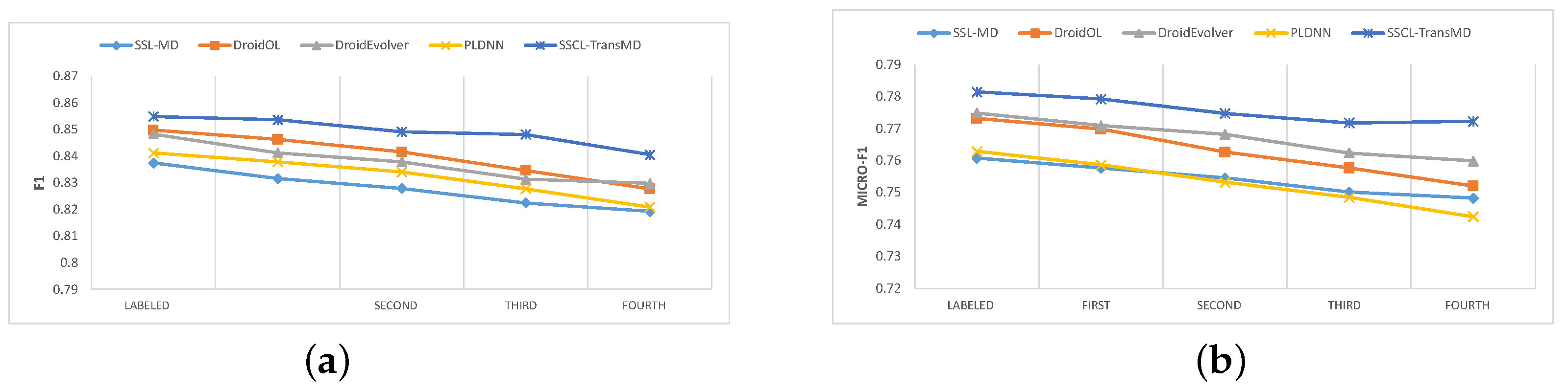
The experiment results are shown below.

Table 9. Binary classification of CICMalDroid2020.

Model	Labeled	First Input of Mixed Samples	Second Input of Mixed Samples	Third Input of Mixed Samples	Fourth Input of Mixed Samples
SSL–MD	0.8375	0.8316	0.8279	0.8225	0.8193
DroidOL	0.8498	0.8463	0.8416	0.8347	0.8278
DroidEvolver	0.8483	0.8413	0.8379	0.8314	0.8298
PLDNN	0.8412	0.8379	0.8341	0.8278	0.8209
SSCL–TransMD	0.8549	0.8537	0.8492	0.8482	0.8406

and

Table 10. Multi-classification of CICMalDroid2020.

Model	Labeled	First Input of Mixed Samples	Second Input of Mixed Samples	Third Input of Mixed Samples	Fourth Input of Mixed Samples
SSL–MD	0.7261	0.7223	0.7198	0.7166	0.7153
DroidOL	0.7407	0.7379	0.7340	0.7301	0.7264
DroidEvolver	0.7396	0.7365	0.7321	0.7287	0.7255
PLDNN	0.7255	0.7214	0.7185	0.7112	0.7076
SSCL-TransMD	0.7528	0.7489	0.7415	0.7355	0.7309

shows the binary and multi-classification results of the methods above respectively.

Among them, when conducting binary classification detection, the F1-score has an average improvement of 1.27% compared to other models. Furthermore, after inputting hybrid samples four times, which include historical labeled samples and new unlabeled samples, the F1-score has an average improvement of 1.96%.

When performing multi-class classification using the CICMalDroid 2020 dataset for labeled training, compared to other models, the Micro-F1 metric saw an average improvement of 2.7%. Furthermore, after inputting a mixture of samples containing historical labeled samples and new unlabeled samples four times, the Micro-F1 metric saw an average improvement of 1.7%.

Through comprehensive analysis, it can be concluded that the proposed SSCL–TransMD detection model in this paper achieves good results in both binary and multiclass classification. Compared to other semi-supervised classification methods SSL–MD and DroidEvolver based on pseudo-labeling, the pseudo-labeling determination method used in our proposed SSCL–TransMD is more effective in improving the model. Compared to other deep learning models DroidOL and PLDNN, the Transformer-based model performs better in the scenario of semi-supervised continual learning.

4.2.2. Analysis of Ablation Experiments

Compared with the Transformer model, the SSCL–TransMD detection model proposed in Section 4 of this paper has three main differences:

1. The addition of parameter $\lambda$ to memorize and replay unlabeled input data and labeled historical data; 2. The adoption of the LLGC algorithm to provide pseudo-labels before training the information encoding component; 3. The usage of the MLP algorithm to decode the Encoder and directly output the classification detection results.

The comparison models used in the ablation experiments are as follows:

1. SSCL–Transformer model: The SSCL–Transformer model adds the MLP algorithm to the Transformer’s encoder to decode and output the classification results. It continuously inputs semi-supervised malicious software data during the ablation experiment training process; 2. SSCL–TransMD model: The SSCL–TransMD model adds the LLGC algorithm to provide pseudo-labels for the Encoder layer in the SSCL–Transformer model, assisting in the computation of the information encoding layer. Other settings are the same as the SS–Transformer model.

This subsection primarily discusses the improvement of the similarity calculation component on the SSCL–TransMD model and proves its effectiveness in the binary classification scenario.

The visualization results for the CICMalDroid 2020 dataset are shown in Figure 4.

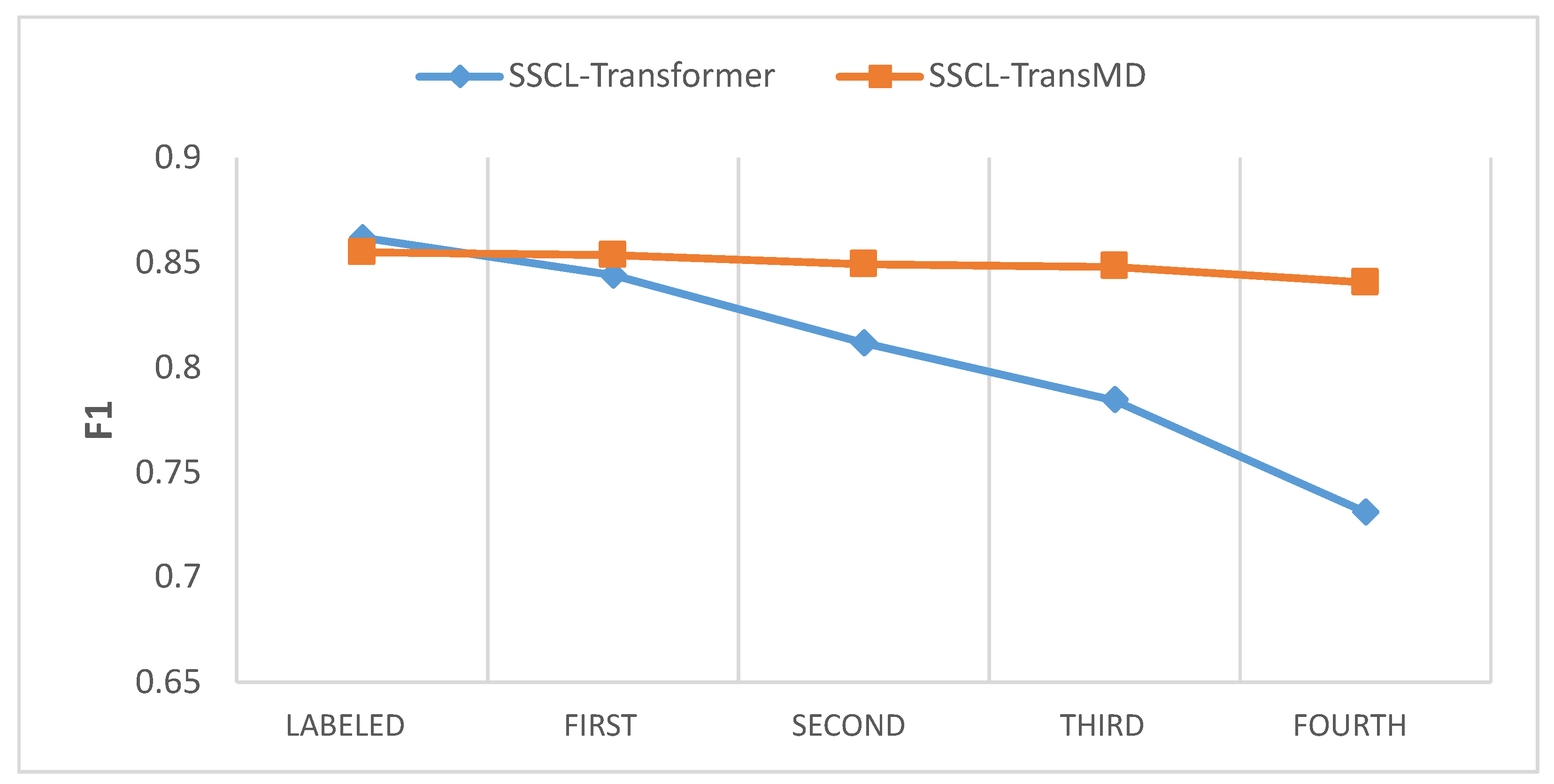
Based on the ablation experiment results in Figure 5 and

Table 11. Results for ablation experiments.

Model	Labeled	First Input of Mixed Samples	Second Input of Mixed Samples	Third Input of Mixed Samples	Fourth Input of Mixed Samples
SSCL–Transformer	0.8618	0.8441	0.8119	0.7846	0.7311
SSCL–TransMD	0.8549	0.8537	0.8492	0.8482	0.8406

, the analysis of the similarity calculation component is as follows.

As a pre-training component of the model, the processing of unlabeled data by the similarity calculation component has a significant impact on the classification accuracy of the model. With the input of unlabeled malware in the CICMalDroid 2020 dataset, it can be seen that the F1-score of the SSCL–Transformer model shows a significant downward trend. After the fourth input, which includes a mixture of historical labeled samples and new input unlabeled samples, the F1-score is, on average, decreased by 20.59% compared to the initially trained F1-score in the three datasets. The F1-score of the SSCL–TransMD model, which calculates similarity scores through the similarity calculation component, decreases by an average of 2.02%. Therefore, intuitively speaking, the similarity calculation component avoids catastrophic forgetting issues.

4.2.3. Model Parameter Sensitivity Analysis

The SSCL–TransMD model for malicious software detection is based on semi-supervised continual learning and contains multiple hyperparameters. Different parameters have a significant impact on the accuracy of malicious software detection. In this section, multiple sets of comparative experiments are conducted on the CICMalDroid 2020 dataset to observe the influence of hyperparameters on the experimental results. The proportion of the training set in the experiment is set to 0.5. All parameters except the one being tested are set to their default values. The selected hyperparameters for this experiment are the baseline weight ${\lambda }_{base}$ in the memory replay component and the number of iterations T in the similarity calculation component.

(1)

Baseline weight ${\lambda }_{base}$

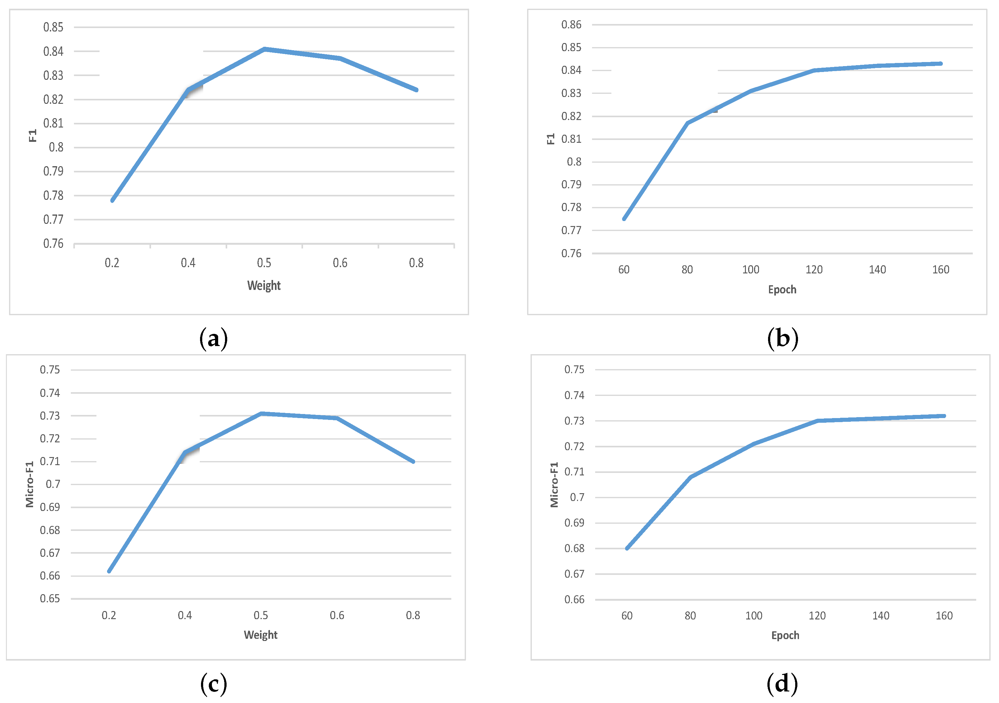
The baseline weight ${\lambda }_{base}$ in the memory replay component determines the adaptive weight ${\lambda }_{new}$, which is the core parameter to address sample imbalance. In this Section, ${\lambda }_{base}$ is successively set to 0.2, 0.4, 0.5, 0.6, and 0.8 for binary classification and multi-classification experiments. Only the metrics after four rounds of mixed-sample training are recorded. The experimental results are shown in Figure 6.

By observing Figure 6a,b, it can be found that, as ${\lambda }_{base}$ increases, the model’s classification accuracy initially increases and then decreases. The highest classification accuracy is achieved when ${\lambda }_{base}$ is 0.5, indicating that sample balance is best achieved when ${\lambda }_{base}$ = 0.5. Therefore, the default value of ${\lambda }_{base}$ in the training process of the SSCL–TransMD detection model is set to 0.5.

(2)

Iteration number T

The iteration number T in the similarity calculation component is a key parameter for calculating the similarity of pseudo-labels. In this Section, we set T to 60, 80, 100, 120, 140, and 160 for binary classification experiment training and multi-classification experiment training. We only record the metrics after four rounds of mixed sample training, and the experimental results are shown in Figure 6c,d.

By observing Figure 6c,d, it can be observed that, as the parameter T increases, the model’s classification accuracy shows an upward trend. However, after 120 iterations, the classification accuracy does not show a significant improvement, indicating that the accuracy of pseudo labels is already close to the true labels at this time. Considering the increasing number of unlabeled samples in subsequent inputs, the iteration number can be appropriately increased. In this paper, considering that the scale of each piece of input unlabeled sample data is similar in SSCL–TransMD detection model, the default value of T is set to 120.

5. Discussion

Continuous learning is one effective way to maintain model learning. However, it also brings some new challenges: (1) it needs stable and high-quality source of samples, which requires enough labeled samples; (2) the fixed structure of deep learning neural networks directly determines the limited capacity of the model, which leads to the result that neural networks forget historical data to learn new data.

To address the aforementioned challenges, we have introduced a novel approach known as semi-supervised continuous learning Transformer malware detection (SSCL–TransMD). In order to mitigate the issue of catastrophic forgetting that often occurs during the training process, we have employed an enhanced version of LUMP. Additionally, we have utilized LLGC to accurately determine the peusdo-label of newly acquired data.

With continuous learning, the proposed method possesses the ability to keep learning new samples, which means that the proposed method is able to detect unknown malware-like samples. Meanwhile, LUMP solves the catastrophic forgetting in the process of continuous learning. Furthermore, because of the incorporation of pseudo-labeling, the continuous learning of the model is no longer confined to high-quality labeled sampled data, thereby significantly enhancing the practicality of the model.

However, there are also some shortcomes in our proposed method. Due to the predominant focus of the method proposed in this article on adapting to unknown samples, the detection accuracy is not high when facing ordinary labeled detection tasks. This aspect can be observed from the first column in Table 9. Also, the proposed model requires more computational resources than the detection models that are only trained once. Based on these two points, we propose two potential future directions: (1) Improve the structure of the detection model to raise the detection rate; (2) Reduce the cost of detection model.

6. Conclusions

With the advent of the smartphone era, the utilization of mobile phones has become increasingly widespread, which leads to the situation that smartphones have become the front line of cyberspace security. Unfortunately, with the evolution of malware detection methods, the malware itself is also incessantly upgrading. This has led to a precipitous decline in the detection rate of many deep learning-based malware detection systems when detecting unknown samples. Continuous learning is one of the solutions to this problem, but, in the process of continuous learning, deep learning models may experience a phenomenon of forgetting what they have already learned, known as catastrophic forgetting. Due to this challenging catastrophic issue of forgetting during model retraining, the field of malware detection still faces immense challenges.

To address the catastrophic forgetting issue during the continuous updating process of malware models, building upon existing theoretical achievements, a malware detection model based on semi-supervised continuous learning (SSCL–TransMD) is proposed. The SSCL–TransMD model first adopts the lifelong unsupervised learning algorithm LUMP as the foundation and introduces modifications, mainly in the weight calculation method, to incorporate adaptive weight calculation. The improved LUMP algorithm is used to dynamically sample a mixture of labeled historical samples and unlabeled new input samples proportionally, thereby alleviating the adverse effects caused by sample imbalance. Furthermore, the LLGC semi-supervised algorithm is employed to iteratively compute similarity scores for the unlabeled samples in the mixture samples, obtaining pseudo-labels. Lastly, an MLP-based neural network is designed to classify malicious software and provide output results. Finally, we evaluated and examined the proposed method on dataset CICMalDroid2020. The results showed that our proposed method significantly outperforms other methods in continuous learning scenarios. More specifically, the deterioration rate of detection performance for the proposed method is significantly lower when facing the continuous input of new samples compared to other methods, which means that SSCL–TransMD can outperform other detection models when encountering unknown samples in a real-world network.

Unfortunately, the detection accuracy of SSCL–TransMD is still not good enough in the scenario of supervised learning. In the future, we will place our attention on improving the detection accuracy.