Semi-Supervised Seizure Prediction Model Combining Generative Adversarial Networks and Long Short-Term Memory Networks

Abstract

In recent years, significant progress has been made in seizure prediction using machine learning methods. However, fully supervised learning methods often rely on a large amount of labeled data, which can be costly and time-consuming. Unsupervised learning overcomes these drawbacks but can suffer from issues such as unstable training and reduced prediction accuracy. In this paper, we propose a semi-supervised seizure prediction model called WGAN-GP-Bi-LSTM. Specifically, we utilize the Wasserstein Generative Adversarial Network with Gradient Penalty (WGAN-GP) as the feature learning model, using the Earth Mover’s distance and gradient penalty to guide the unsupervised training process and train a high-order feature extractor. Meanwhile, we built a prediction model based on the Bidirectional Long Short-Term Memory Network (Bi-LSTM), which enhances seizure prediction performance by incorporating the high-order time-frequency features of the brain signals. An independent, publicly available dataset, CHB-MIT, was applied to train and validate the model’s performance. The results showed that the model achieved an average AUC of 90.08%, an average sensitivity of 82.84%, and an average specificity of 85.97%. A comparison with previous research demonstrates that our proposed method outperforms traditional adversarial network models and optimizes unsupervised feature extraction for seizure prediction.

1. Introduction

Epilepsy is a common neurological disorder characterized by the abnormal discharge of neural cells in the brain [1], leading to functional disturbances. It is characterized by recurrent, sudden, and temporary abnormalities in motor, sensory, emotional, behavioral, or mental symptoms. Epilepsy affects nearly 50 million people worldwide [2], with approximately 30% of patients unable to control their condition with medication. Early prediction of seizures is an important factor in effective treatment and management of epilepsy [3], as it can help prevent patients from engaging in potentially dangerous activities during seizure-free periods. Improving the accuracy of seizure prediction can greatly enhance the quality of life for patients and enable more effective preventive treatments.

An electroencephalogram (EEG) is currently an effective diagnostic tool for epilepsy, as it can record abnormal brain activity associated with seizures [2]. However, the manual labeling and retrospective analysis of EEG signals by doctors is time-consuming and prone to errors due to the random and non-stationary nature of EEG signals [4,5,6]. Additionally, there are individual differences in EEG data among patients, and the occurrence of seizures in epilepsy patients is highly uncertain, with each patient having different seizure patterns and timing. Furthermore, EEG signals are often contaminated by other normal brain activities [7]. Therefore, seizure prediction based on EEG is still a challenging task [8].

In the past 20 years, computer-assisted epileptology research has gradually been applied to epilepsy classification and seizure prediction. Early seizure prediction methods mainly relied on thresholding techniques, where an increase or decrease in specific features was used to predict an impending seizure [9]. However, there is no unified standard feature for detection, making it difficult to achieve accurate predictions. More researchers have proposed using machine learning for seizure prediction. These algorithms mainly focus on combining feature extraction and classifier performance, showing relatively good results in detecting pre-seizure states [10,11,12,13,14]. However, these algorithms often require individualized analysis due to significant differences in seizure patterns among patients, making the process complex and impractical for wider applications [15,16,17]. Deep learning methods, on the other hand, can automatically extract features and train classifiers end-to-end, greatly improving feature extraction and achieving better classification results [18,19,20,21]. However, these algorithms require a large amount of labeled EEG data for training, which relies on the diagnostic experience of clinical doctors and is a time-consuming and subjective process.

Although significant progress has been made in the analysis of epilepsy using the above-mentioned methods, analyzing brain electrical signals still faces complexity and challenges. Firstly, due to the large differences between patients, it remains a very difficult task to differentiate between pre-ictal and interictal states in different patients, even for experienced medical experts. Secondly, the robustness of the models used is poor, sometimes resulting in lower performance for another patient when a model with an AUC score of 1 is used for a different patient, resulting in a lower score of 0.3 [19]. This fluctuation makes the model unreliable for other patients. Finally, due to the limitations of seizure disorders, obtaining labeled data before seizures is not readily available, which limits the availability of training data for machine learning and further restricts the predictive accuracy and generalizability of traditional machine learning models.

Unsupervised feature learning has emerged as a promising direction for the application of deep learning in seizure prediction. It overcomes the difficulties of requiring a large amount of labeled data. More and more people are using unsupervised feature learning with unlabeled data, such as clustering, Gaussian mixture models, hidden Markov models, and autoencoders [22,23]. Unsupervised learning does not rely on any labels and instead exploits the inherent structural properties of the data to perform relevant tasks. It can be applied during the recording of EEG signals, eliminating the need for data annotation and individual feature extraction methods for each patient. This technique has mainly been used in seizure detection and has achieved high sensitivity and specificity [22,24,25]. Currently, there are two main techniques utilized: autoencoders (AE) and deep convolutional generative adversarial networks (DCGAN) [26,27,28,29,30]. However, there is relatively limited research on successfully applying unsupervised learning to seizure prediction. In a study [26], the authors used unsupervised stacked autoencoders (SAE) combined with prior knowledge to extract features and train a SVM classifier, achieving a sensitivity of 95% and a false positive rate (FPR) of 0.06/h. Unfortunately, this result was only tested on intracranial EEG signals from two patients, and the performance impact of the features extracted from SAE could not be determined due to the use of prior knowledge in feature design. In another study [31], researchers tested their method on the CHB-MIT dataset, using a deep convolutional autoencoder to extract features and input them into a bidirectional long-short-term memory model, ultimately achieving a sensitivity of 94.6% and an FPR of 0.04/h. However, this method had a seizure prediction horizon (SPH) of 0, which means there was no reserved time for clinical intervention, resulting in a lack of practical utility.

In response to the given questions, this paper proposes a predictive model called WGAN-GP-Bi-LSTM. The model combines the Short-Time Fourier Transform (STFT), a Wasserstein Generative Adversarial Network with Gradient Penalty (WGAN-GP), and a semi-supervised epileptic seizure prediction algorithm based on the Bi-LSTM classification network model.

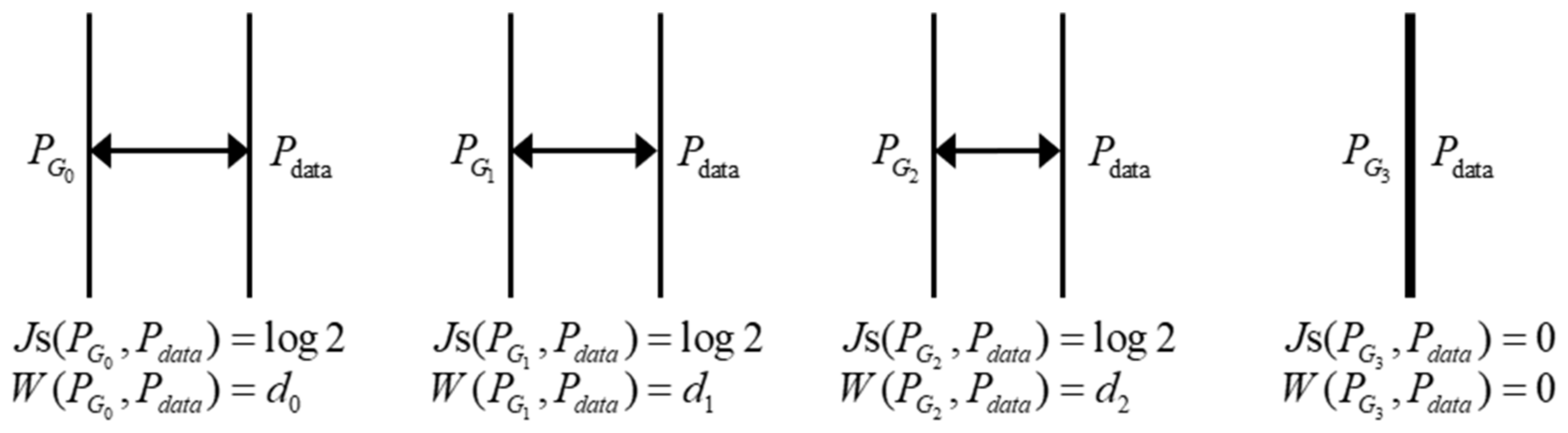
Firstly, the time series data of the EEG signals is transformed into a two-dimensional matrix with time and frequency axes using the STFT. Secondly, the WGAN-GP is used as an unsupervised feature learning model. This model uses Earth-Mover (EM) distance as a measure instead of Jensen-Shannon (JS) divergence to overcome training instability and model collapse issues, ensuring the richness of generated samples [32,33]. Lastly, a Bi-LSTM classification model is employed as the backend classifier, using a small amount of labeled STFT spectrograms to guide the prediction task. This classification model efficiently captures temporal information in EEG signals, thereby improving prediction performance [34].

The proposed methodology is validated on the publicly available CHB-MIT dataset of pediatric epilepsy data. The performance of the proposed method is evaluated using metrics such as AUC, sensitivity, and specificity.

The contributions of this paper are as follows:

• Introducing the WGAN-GP model for unsupervised feature learning of epileptic EEG signals. Although WGAN-GP is commonly used in machine learning models, its application in EEG signal feature extraction, especially for epileptic seizure prediction, is limited.
• Using semi-supervised learning methods to compensate for the deficiencies of fully supervised and unsupervised learning methods.
• Validation of the proposed method using the CHB-MIT dataset, demonstrating its effectiveness through measurements of AUC, sensitivity, and specificity.

2. Materials and Methods

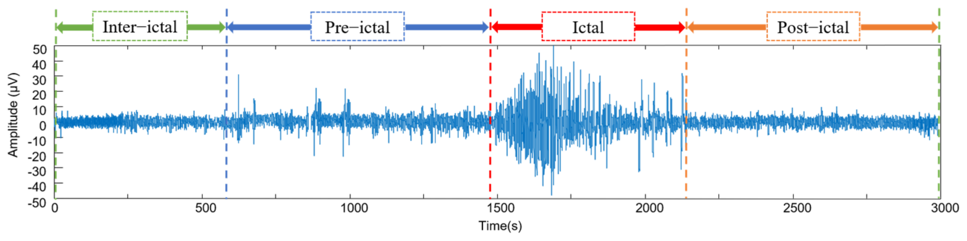
Seizure prediction typically involves recording the patient’s EEG signals in four states: interictal, preictal, ictal, and postictal [10,35] (Figure 1). The interictal period represents the normal brain state, far from seizure activity. Prior to a seizure, the patient’s EEG signals exhibit abnormal fluctuations, known as the preictal phase. The preictal phase transitions from a normal state to a seizure state. The ictal period corresponds to the actual occurrence of a seizure. The postictal phase refers to the transitional period when the brain returns to its normal state after a seizure. Seizure detection based on EEG signals aims to distinguish between the interictal and ictal periods, while seizure prediction focuses on analyzing the preictal state of the EEG signals, specifically performing classification tasks between the preictal and interictal periods.

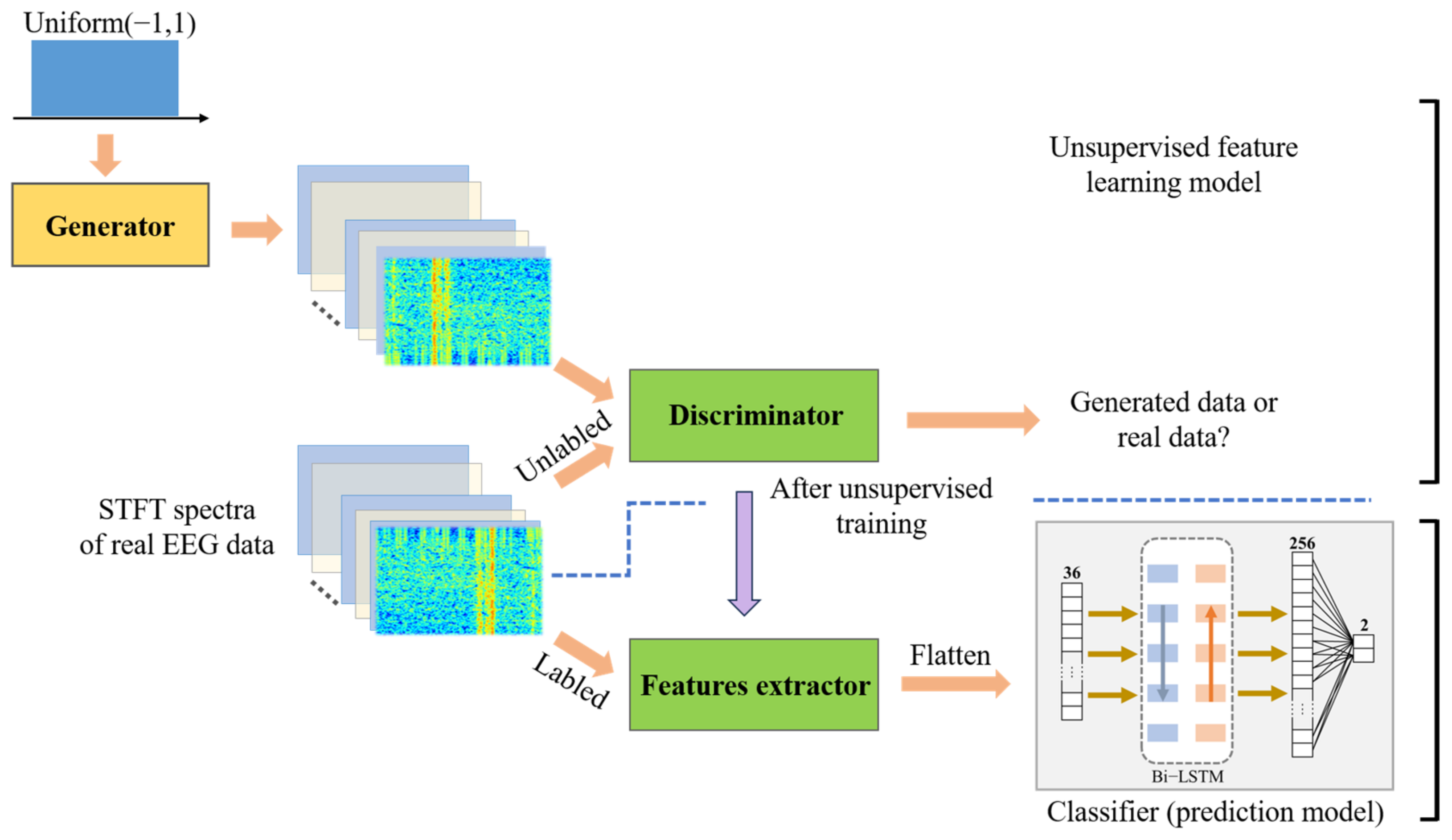
The algorithmic process of this study is shown in Figure 2, which mainly includes: (1) Training of the unsupervised feature learning model (WGAN-GP): The unlabeled EEG signals are transformed into two-dimensional time-frequency feature maps using a short-time Fourier transform. Combined with the patient data in the database, the WGAN-GP model is trained to generate a high-performance feature extractor. (2) Training of the classifier model: The trained WGAN-GP discriminator is used as the feature extractor, combined with Bi-LSTM to construct a classification network. A small amount of labeled EEG signals with STFT time-frequency maps is used to train the classifier model and complete the classification task.

There are three commonly used techniques for analyzing brain signals: time domain analysis, frequency domain analysis, and time-frequency domain analysis [10]. Time domain analysis examines the voltage amplitude of the signal over time, while frequency domain analysis examines the spectral distribution and energy changes of the signal in the frequency domain. Both time and frequency domain analysis methods are typically effective for analyzing stationary signals and can only reflect single signal characteristics, which are not suitable for extracting nonlinear features of brain signals. Time-frequency analysis combines time and frequency domain calculations to describe the frequency information of a signal over a period of time, making it a common method for processing EEG signals.

The STFT is a commonly used tool in signal processing. It involves dividing a longer time signal into shorter segments of equal length and then calculating the Fourier transform, or Fourier spectrum, of each segment to obtain the frequency changes over time. The mathematical formula for a single-channel EEG signal $x(t)$ can be represented as follows:

$$STFT(f,t)={\displaystyle {\int }_{-\infty }^{+\infty }[x(t)g(t-\tau )]e^{-j2tf\tau }d\tau },$$

(1)

In (1), $t$ represents the time point, $f$ is the frequency component in the signal, and $j$ represents the imaginary unit. $x(t)$ represents the time series of the EEG signal, $g(t)$ represents the window function, and $\tau$ represents the index of different time windows.

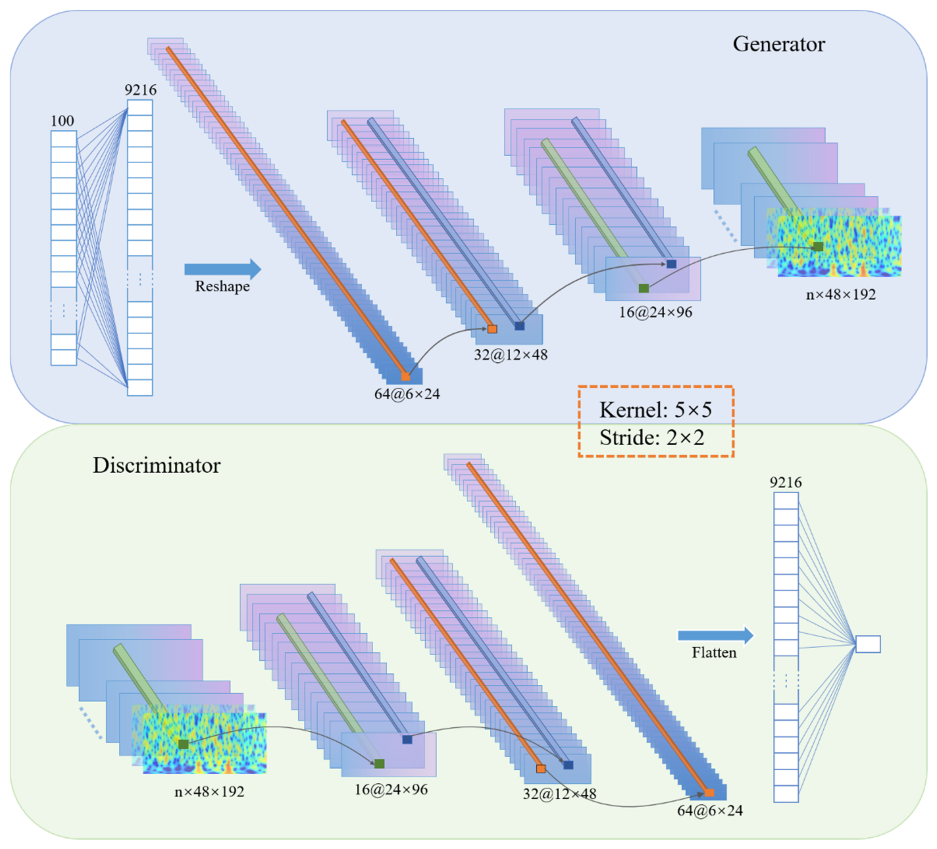
2.1. Training Generative Adversarial Networks

Generative adversarial networks (GANs) are a novel type of unsupervised learning model that has shown better performance compared to traditional neural network models, making them one of the hottest artificial intelligence technologies in recent years. GANs were first proposed by Ian J. Goodfellow et al., in October 2014 [36] and have since been widely applied in the field of image processing.

GANs consist of two components: the generator and the discriminator. The generator takes random noise as input to generate images, while the discriminator is responsible for judging whether the input image is real or fake by outputting the probability of the image being real. A smaller probability indicates a higher likelihood of the generated image being fake.

The goal of the generator is to generate more realistic images to deceive the discriminator and increase the probability of being classified as real. On the other hand, the discriminator aims to distinguish between real and fake images and lower the probability of being classified as real. Through this dynamic game process, a Nash equilibrium is reached, and training is performed using deep neural networks [37]. The objective function of GANs is defined as:

$$\underset{G}{\min } \underset{D}{\max }V(D,G)={{\rm E}}_{x\sim p_{data}(x)}[\log D(x)]+{{\rm E}}_{z\sim p_z(z)}[\log (1-D(G(z)))],$$

(2)

In (2), data represents real data, $p_{data}$ represents the distribution of the real data, $z$ represents random noise (input data), $p_z$ represents the distribution of the original noise, $G()$ represents the generator mapping function, and $D()$ represents the discriminator mapping function. The generator and discriminator models compete against each other to reach a global optimum. Specifically, given $G$, the goal is to maximize the evaluation of the distance between $p_G$ and $p_{data}$ using $V(D,G)$. $p_G$ represents the data distribution obtained after generating data using the generator.

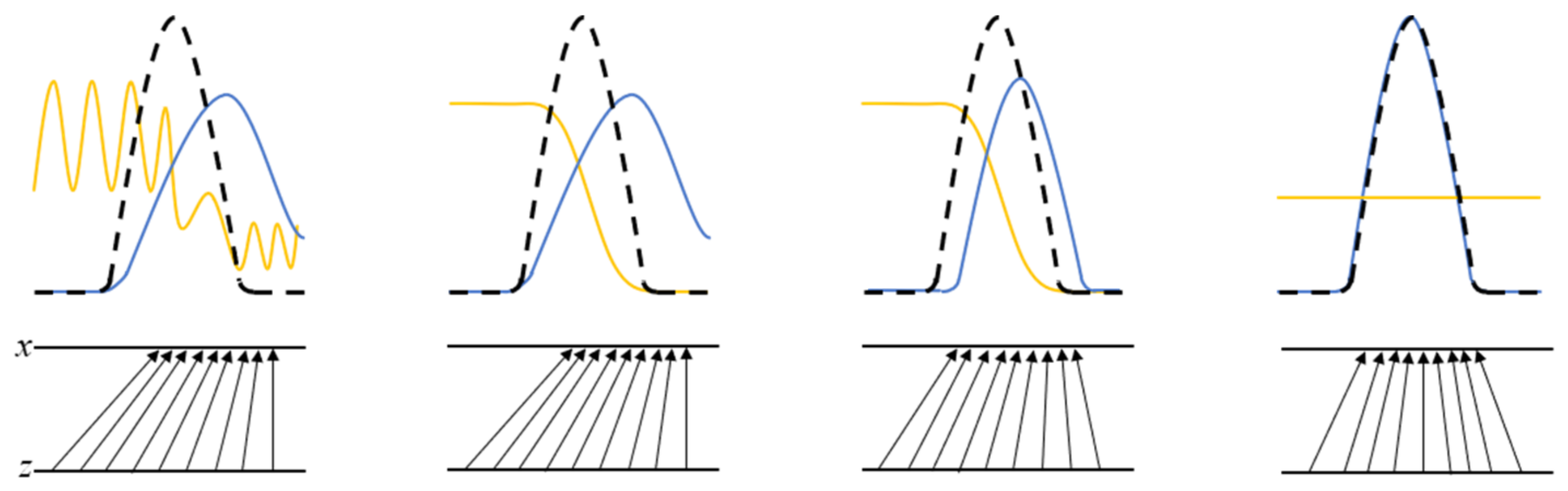
As shown in Figure 3, the yellow solid line represents the discriminative distribution, while the black dashed line and the blue solid line represent the generated real and fake samples, respectively. The horizontal line z is the sampled region. The upward arrow represents the mapping relationship of $x=G(z)$, and $G$ contracts in the high-density area of $p_G$ while expanding in the low-density area. When $G$ and $D$ reach a point where neither can improve, the discriminator is unable to distinguish between the two distribution classes.

WGAN-GP Feature Extraction Model

The generator and discriminator of the traditional GAN model, guided by the loss function, continuously play the game of max-min and update by learning against each other until the output is 0.5, at which point the network reaches a stable state and ends the training. The generator’s loss function is denoted as $G_{loss}$, while the discriminator’s loss function is denoted as $D_{loss}$. The definitions are as follows:

$$D_{loss}=\frac{1}{m}{\displaystyle \sum _{i=1}^m[\log D(x^{(i)})+}\log (1-D(G(z^{(i)})))],$$

(3)

$$G_{loss}=\frac{1}{m}{\displaystyle \sum _{i=1}^m\log (1-D(G(z^{(i)})))},$$

(4)

In Equations (3) and (4), $m$ is the batch size of 64, $x$ is the original STFT of the EEG signal, and $z$ is sampled from the distribution $U(-1,1)$. When the network is stable, the data generated by the generator is close to the real time-frequency distribution, and the discriminator has feature extraction ability; that is, the network layers of the discriminator form a feature extractor [28]. Therefore, network training is crucial for improving feature extraction abilities.

However, traditional GANs suffer from problems of gradient vanishing and unstable training [30,38]. As shown in Figure 4, the generator minimizes the Jensen-Shannon divergence (JS divergence) between the generated distribution $p_G$ and the real distribution $p_{data}$ using a loss function. The definitions are as follows:

$$JS(P_G‖P_{data})=\frac{1}{2}{\displaystyle \sum P_G(x)\log (\frac{P_G(x)}{P_G(x)+P_{data}(x)})}+\frac{1}{2}{\displaystyle \sum P_{data}(x)\log (\frac{P_{data}(x)}{P_G(x)+P_{data}(x)})+\log 2},$$

(5)

When there is little or no overlap between the two distributions, the JS divergence is constant, causing the discriminator to quickly converge, leading to the gradient vanishing. Additionally, during the training process, if the generator and discriminator cannot converge simultaneously, it can result in mode collapse, making the training process unstable.

Therefore, this paper adopts WGAN-GP to improve the above-mentioned issues. WGAN-GP is an improved model based on WGAN, with the core being the replacement of the evaluation method for measuring the distance between the generated distribution and the real distribution. In WGAN, the Wasserstein distance is used, which replaces the JS divergence that is not suitable for measuring the distance between non-overlapping parts of the distributions [39]. Compared to JS divergence, the Wasserstein distance can reflect the distance between distributions when there is no overlap in the data distribution. Additionally, the Wasserstein distance has a continuous and smooth change, allowing for optimization of model parameters using gradient descent. By adding gradient penalty (GP) to WGAN, the training speed and the quality of generated samples are improved, further overcoming the problem of slow convergence in network training.

The WGAN-GP model structure used in this study is illustrated in Figure 5. The generator takes a 100-dimensional sample from a uniform distribution $U(-1,1)$ as input. The input is then fully connected to a hidden layer with 9216 nodes, which is reshaped into a 64 × 6 × 24 tensor. After the hidden layer, three deep deconvolutional layers are connected, which increase the dimensions of the input by extending its length and width while reducing the depth until the last layer reaches the desired dimension. The number of filters in these deconvolutional layers is 32, 16, and n, where n = 16 represents the number of channels in the EEG data. The filter stride is 2 × 2, and the filter size is 5 × 5. The output of this generator has the same dimensions as the short-time Fourier transform of a 28-s EEG signal.

The discriminator is composed of three convolutional layers, each with a filter size of 5 × 5 and a stride of 2 × 2. The respective numbers of filters in these layers are 16, 32, and 64. Throughout the training process, signals that bear resemblance to the original signal are generated by the generator. Optimization of the results is achieved by the discriminator through parameter adjustments in the convolutional layers. Features from the epileptic EEG signals are learned and extracted, culminating in the detection and differentiation between real and fake data.

2.2. Bi-LSTM Classifier Model

After establishing the unsupervised feature learning model, the classifier autonomously learns discriminative features to classify the pre-ictal and inter-ictal data. Recurrent neural networks (RNNs) differ from other types of neural networks as they can maintain the state between different sequential inputs and can independently process a set of time series data. A complete RNN consists of the same feedforward neural network (RNN cells), and each step corresponds to a time.

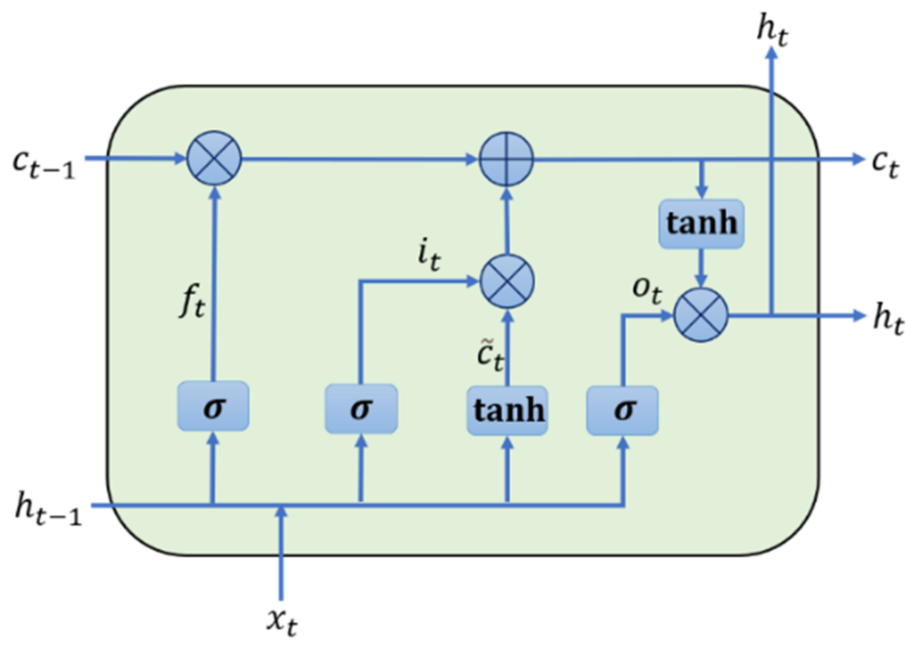
LSTM is a special type of RNN used to overcome the problems of gradient vanishing and information distortion during neural network training. It can easily learn long-term dependencies. LSTM introduces the concept of memory cells with control gates. LSTM not only maintains gradient values during training but also preserves the temporal dependencies between inputs. Figure 6 illustrates the structure of a single LSTM cell.

In this context, $x_t$ represents the input at time $t$, while $f_t$, ${\tilde{c}}_t$, and $o_t$ represent the forget gate, input gate, and output gate, respectively. $h_{t-1}$ and $c_{t-1}$ are the shadow and cell states from the previous step. $h_t$ and $c_t$ represent the next state transferred to the next cell.

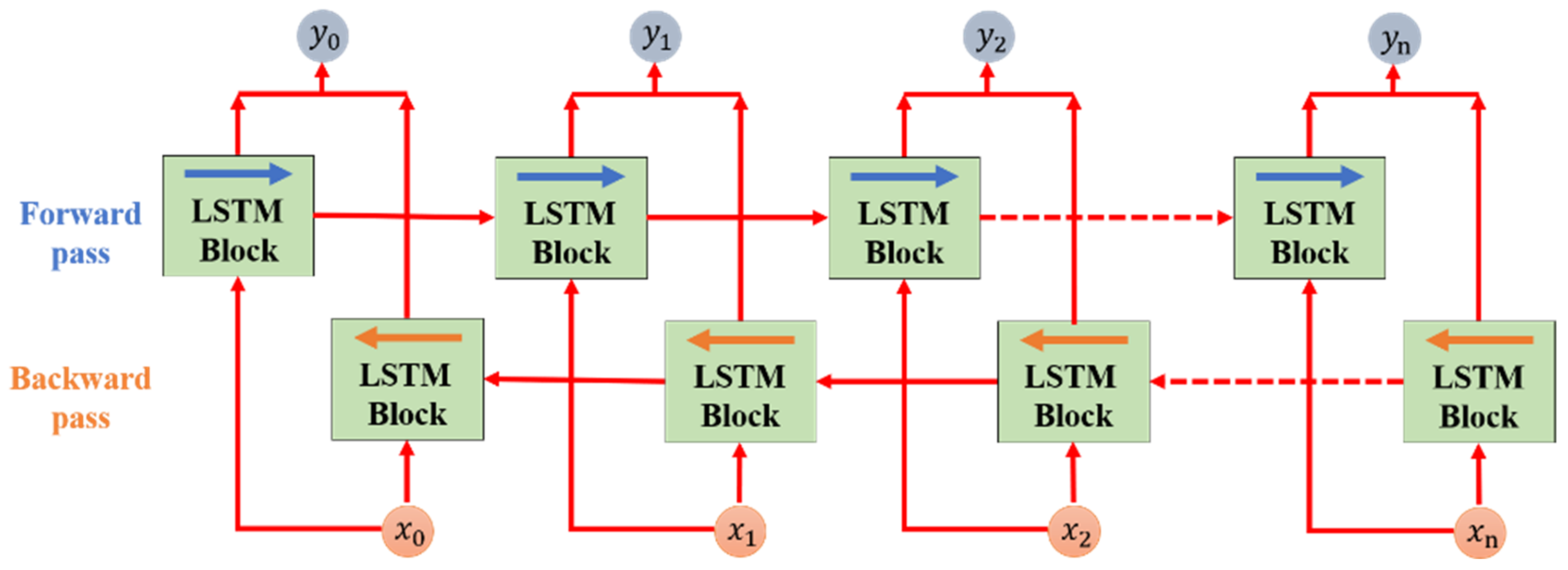
An LSTM block consists of one or more LSTM cells, and each cell processes a time sequence continuously in one direction. At a particular time point, the LSTM block only calculates new state information based on the previous state and current input and outputs it to the next LSTM block until the last input is processed and the output is computed, completing the task. This type of LSTM network is called unidirectional LSTMs.

The Bi-LSTM network is an optimized version based on the LSTM. In the Bi-LSTM, a single layer consists of two LSTM blocks that process two sequences of inputs in opposite directions, as shown in Figure 7. The results of the two LSTM blocks in a single layer are combined to compute the final output for the task at hand. The Bi-LSTM takes into account the temporal dependency of the input data, which makes it promising for achieving higher classification results.

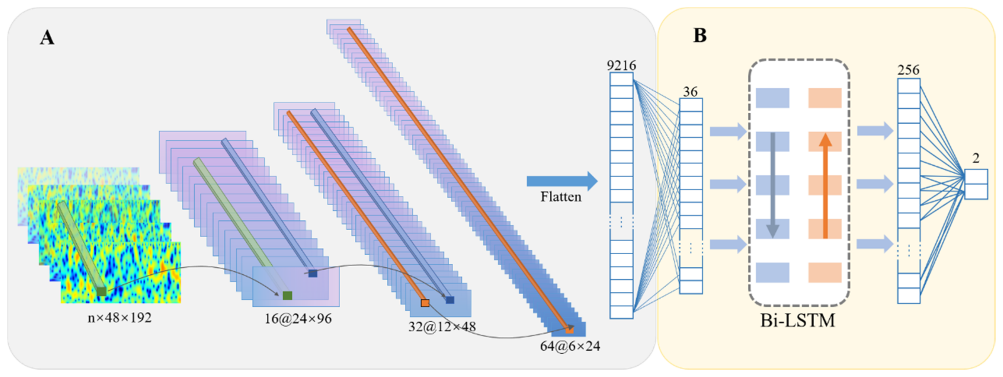
Figure 8 illustrates the construction of the classifier module: the classification network flattens the features extracted by the feature extractor and connects them to a fully connected layer. To reduce the computational complexity of the classification network, the feature vector is mapped to a 36-dimensional space. Furthermore, a Bi-LSTM layer is added to extract temporal features, followed by two additional fully connected layers for further feature extraction. The former uses a sigmoid activation function with an output size of 256, while the latter uses a soft-max activation function with an output size of 2.

2.3. System Evaluation

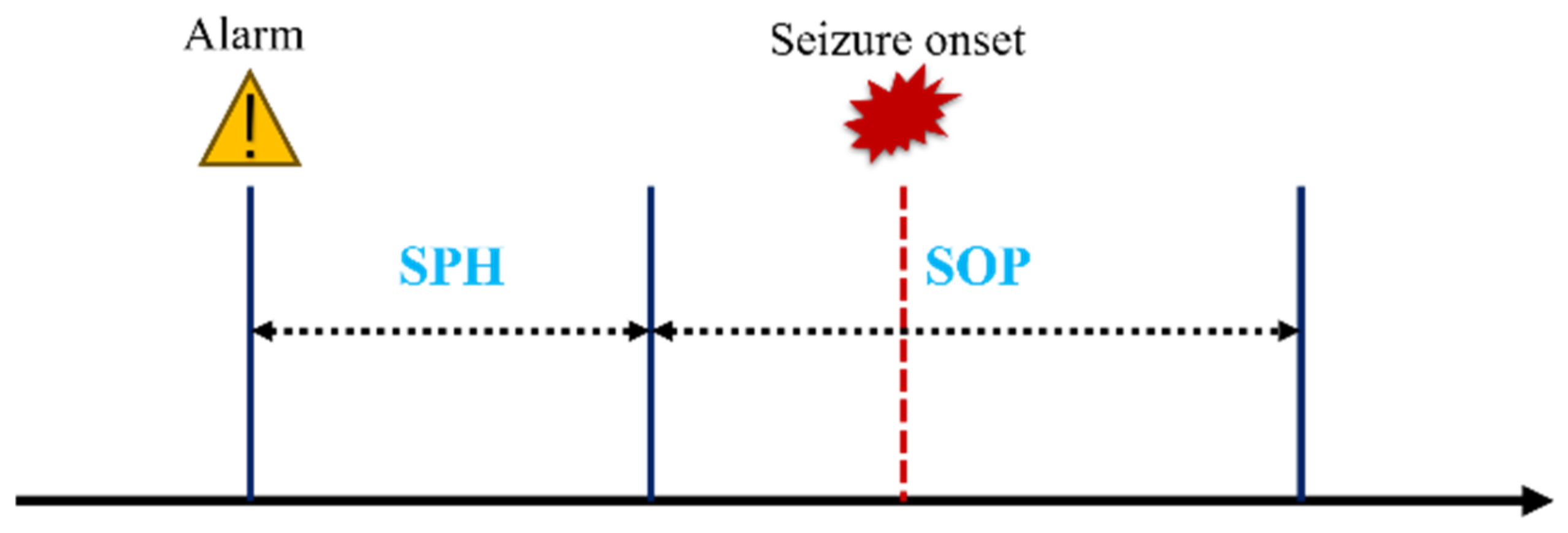
In order to assess the performance of the system, researchers have defined two important time parameters: Seizure Prediction Horizon (SPH) and Seizure Onset Period (SOP). SOP refers to the time period during which a seizure is predicted to occur, while SPH refers to the period from when the prediction alarm is issued to the start of SOP (Figure 9).

Based on this test, the algorithm issues warnings in the form of false alarms or true alarms. This prediction range is set before the onset of seizures, ranging from a few minutes to a few hours. When a disease outbreak occurs outside the SPH range but within the SOP range, it is considered a correct prediction [40]. Any other state is considered an incorrect prediction. The SPH setting should take into account the time needed for clinical intervention and protective measures while also considering the patient’s anxiety levels. In this study, the SPH was set at 5 min and the SOP was set at 30 min, based on relevant research.

3. Experiment and Results

The improved semi-supervised seizure prediction model proposed in this study was implemented and tested using the TensorFlow framework. Training was performed using an NVIDIA GeForce RTX 4090 graphics processing unit (GPU) with 64 GB of memory. The proposed prediction model was trained in two steps: first, unsupervised feature model training, where the feature learner trained through unsupervised learning was combined with a classification network to form a classification (prediction) model for supervised training.

3.1. Dataset

The dataset used in this study is the CHB-MIT dataset [41], which is a collaborative project between Boston Children’s Hospital and MIT. It consists of 23 pediatric patients with 163 seizures and 844 h of continuous scalp electroencephalogram (sEEG) data. The data was sampled at a frequency of 256 Hz and recorded from 22 electrodes.

In order to meet the research objectives of this study, specific selection criteria were applied to the patients:

• Patients who experienced less than ten seizures per day were chosen for the prediction task. Patients with a high frequency of seizures require real-time monitoring and surgical intervention, making them less suitable for seizure prediction.
• At least 30 min of available data before the seizure event were required. In some cases, the time interval between seizures was too short, making it difficult to gather enough pre-seizure training data. Therefore, for seizures with intervals less than 30 min, they were considered a single seizure, and the time of the first seizure was used. Additionally, reserving an appropriate interval between seizures allows for sufficient time for clinical intervention.

Based on these criteria, 13 patient datasets were selected from the CHB-MIT dataset for model validation (

Table 1. Thirteen patients were used in this paper.

Patients	Gender	Age (Years)	No. of Seizures
Patient 1	Female	11	7
Patient 2	Male	11	3
Patient 3	Female	14	7
Patient 5	Female	7	5
Patient 9	Female	10	3
Patient 10	Male	3	7
Patient 13	Female	3	8
Patient 14	Female	9	7
Patient 18	Female	18	6
Patient 19	Female	19	3
Patient 20	Female	6	6
Patient 21	Female	13	4
Patient 23	Female	6	3

).

3.2. Evaluation Indicators

To ensure a thorough evaluation, we utilized the leave-one-out cross-validation approach for each individual patient. The evaluation criteria employed in this research encompassed metrics such as AUC, sensitivity, and specificity. AUC represents the area under the curve and serves as an indicator of the model’s classification capability. Sensitivity and specificity, on the other hand, assess the accuracy of preictal prediction during the interictal period. The value for this particular metric was determined by examining all seizure prediction scores within the leave-one-out cross-validation for each patient.

$$Sensitivity=\frac{TP}{TP+FN},$$

(6)

$$Specificity=\frac{TN}{TN+FP},$$

(7)

$$AUC=\frac{{\displaystyle \sum {(p_i,n_j)}_{p_i>n_j}}}{P\times N},$$

(8)

In Equations (6) and (7), true positive (TP) refers to correctly classified pre-ictal periods, false negative (FN) refers to misclassified interictal periods, true negative (TN) refers to correctly classified interictal periods, and false positive (FP) refers to misclassified pre-ictal periods. In (8), $P$ represents the number of positive samples, $N$ represents the number of negative samples, $p_i$ represents the prediction score for positive samples, and $n_j$ represents the prediction score for negative samples.

3.3. Preprocessing

Based on the analysis of patient data availability, some patients have less than 22 EEG channels. Pat13 and Pat17 have only 17 available channels; Pat4 and Pat9 have 20 and 21 available channels, respectively. In order to ensure the data can be merged, improve data effectiveness, and reduce computational complexity, this study adopts automatic channel selection to retain 16 effective channel data for each patient. The STFT is used to transform each 28-second EEG signal into a two-dimensional matrix consisting of a frequency axis and a time axis. Combining with the epileptic EEG signal annotated by clinical doctors second by second, this study first uses a cosine time window with a length of 1 s and 50% overlap, with a sampling rate of 256 Hz. The signal is filtered to remove 60 Hz power frequency interference based on the local power frequency of data acquisition. The data is trimmed to make the final dimension of each 28-second data (channel number × X × Y) = (16 × 56 × 112), where X and Y are the time and frequency dimensions, respectively.

3.4. Analysis and Experimental Results on Network Stability

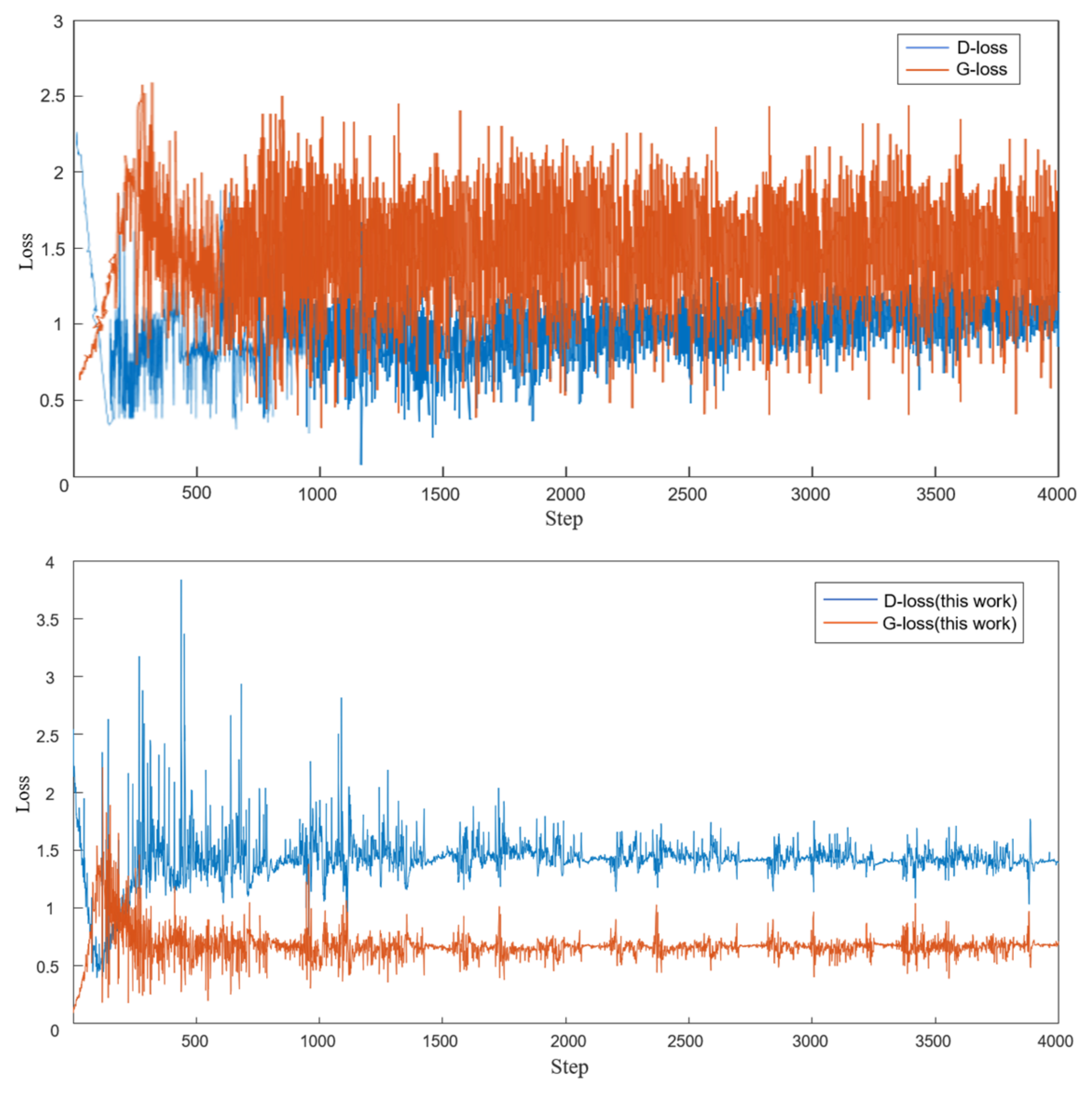
The principle of training GANs is to make the generator and discriminator compete with each other until they reach a balance. When initially training WGAN-GP, the discriminator converged quickly, making it difficult for the generator to learn enough to generate high-quality STFT samples. This resulted in a simple classification of real and fake samples. To overcome this problem, we updated the generator twice and set up an early stopping monitor to track the loss values of the generator and discriminator. If the value of D_loss is greater than G_loss for K consecutive training batches, we stop training WGAN-GP. In this study, we set K = 20, batch size = 64, and the number of training iterations = 10. We also used an Adam optimizer with a learning rate of 1 × 10⁻⁴, λ = 10, β1 = 0.5, β2 = 0.99, and ε = 1 × 10⁻⁸ to optimize the model’s gradients. The training process did not provide any labels for pre-ictal or inter-ictal periods to the network, so the network underwent unsupervised training for epileptic seizure detection.

By visualizing the loss values, we can verify the effects of updating the generator twice. In Figure 10, we plot the initial and updated loss values of the generator and discriminator, using patient 1 from the CHB-MIT dataset as an example. From the graph, we can observe that the updated G_loss value is lower, and the fluctuations are significantly reduced. This means that the generated STFT samples are closer to the original samples, and a better discriminator helps improve its discriminatory performance. The generator and discriminator reached a balance after approximately 1500 steps, at which point the monitor stopped training.

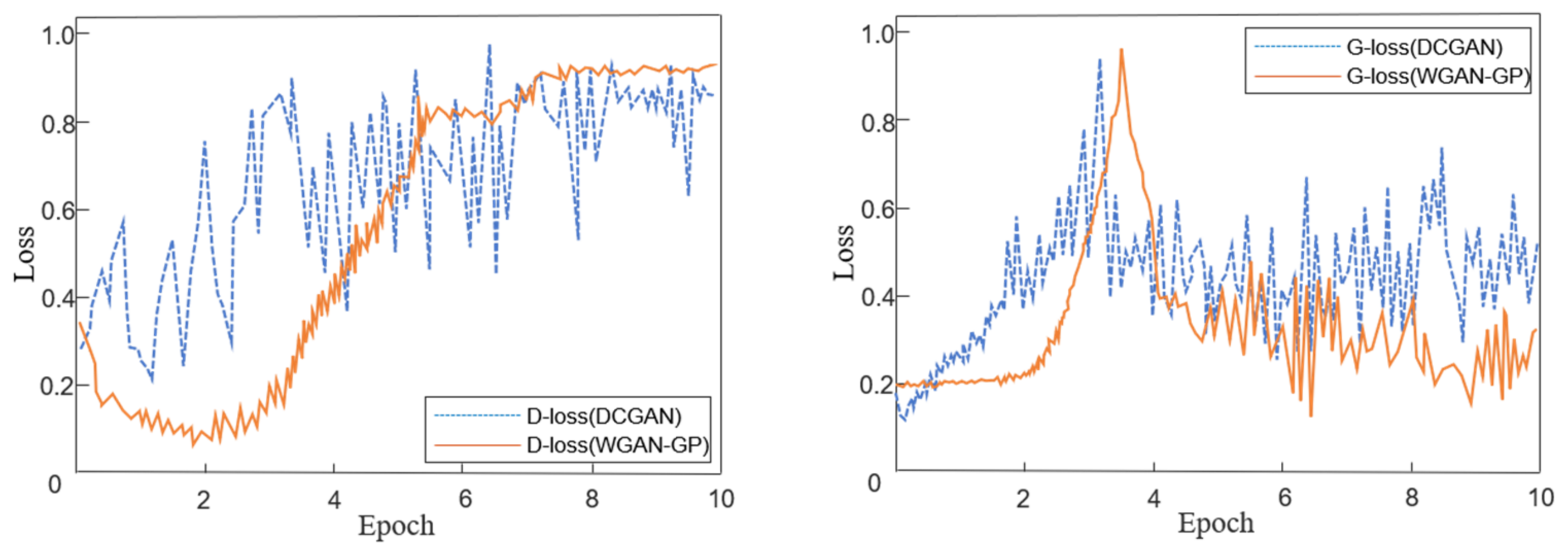
The stability of GAN training is closely related to the variations of D_loss and G_loss and their corresponding gradient changes [33]. Therefore, on the premise of performing STFT preprocessing on the EEG signals, the stability of network iteration training for DCGAN and WGAN-GP generators and discriminators is compared. Figure 11 shows the convergence of D_loss and G_loss after training with two different models on patient 20. Comparing the two, it can be observed that the loss function curve of WGAN-GP has a much smaller oscillation amplitude than DCGAN, and its gradient change trend is also smoother than DCGAN.

Table 1 and

Table 2. Comparison of seizure prediction performance sensitivity (%) on the CHB-MIT dataset under different unsupervised learning models.

Patients	CNN	DCGAN	WGAN-GP	WGAN-GP-BI-LSTM
Patient 1	85.7	92.53	97.23	98.80
Patient 2	33.3	32.25	40.86	83.46
Patient 3	100	21.33	85.64	50.10
Patient 5	80.0	45.67	50.38	82.81
Patient 9	50.0	77.91	80.02	83.93
Patient 10	33.3	68.61	66.27	74.29
Patient 13	80.0	59.60	78.31	82.06
Patient 14	80.0	59.88	51.72	39.67
Patient 18	100	82.22	83.19	95.22
Patient 19	100	57.50	91.28	93.61
Patient 20	100	95.00	94.37	95.42
Patient 21	100	98.22	99.78	100
Patient 23	100	96.00	94.99	97.53
Range	[33.3, 100]	[21.33, 98.22]	[40.86, 99.78]	[39.67, 100]
Average	81.2	68.21	78.01	82.84

provide a comparison of the sensitivity and AUC values for the selected semi-supervised learning method WGAN-GP, the fully supervised learning method CNN, and the semi-supervised learning method DCGAN. From the data in columns 2–4 of Table 1 and Table 2, it can be observed that the WGAN-GP semi-supervised learning method has a 3.19% lower sensitivity compared to the fully supervised learning method. However, it is worth mentioning that WGAN-GP shows a 1.88% improvement in AUC compared to the fully supervised method (CNN). Under the same data preprocessing and model parameter settings, the WGAN-GP semi-supervised method has an average improvement of 9.8% in sensitivity and 13.14% in AUC compared to DCGAN.

To ensure the stability of the classifier training and accelerate convergence, batch normalization is applied at each layer of the network, and the network parameters for high-order feature learning are fixed. To prevent overfitting, the dropout rate for the subsequent two layers of the neural network is set to 0.3. Moreover, 75% of the pre-seizure and inter-seizure samples in the training dataset are used as the training set, while 25% are used as the validation set. To evaluate the performance of the Bi-LSTM as a classifier, we compare it with the WGAN-GP model, which uses fully connected layers for classification.

By comparing the data in columns 4–5 of Table 1 and Table 2, it can be observed that after the same preprocessing and unsupervised feature learning training, the backend classifier using Bi-LSTM achieves a 4.31% higher AUC and a 4.83% higher sensitivity compared to the one using fully connected layers. This result demonstrates that using a Bi-LSTM classifier can improve predictive performance for epileptic seizures.

4. Discussion

This study presents a feature extraction method for epilepsy prediction using an unsupervised training model. While it reduces sensitivity by 3.19% compared to supervised learning, this unsupervised feature extraction method can help minimize the costly and time-consuming task of labeling EEG signals. The unlabeled EEG signals are used to train the WGAN-GP, and the trained discriminator is used as a feature extractor input for the Bi-LSTM classifier for epilepsy prediction.

Compared to supervised learning, semi-supervised learning methods still have a performance gap in epilepsy prediction. Some studies suggest that this gap can be improved by increasing the training size [28]. Oversampling the inputs during the training of the adversarial network helps fill in the data gaps of patients and improves overall epilepsy prediction performance. Therefore, we can infer that the more EEG data available, the higher the prediction accuracy. The advantage of using unsupervised feature extraction is that data recording and feature extraction can be carried out simultaneously without requiring additional effort from clinical doctors.

This research demonstrates that utilizing the Wasserstein distance and gradient penalty can further improve the stability of the unsupervised feature learning model and enhance the quality of time-frequency image generation. Figure 11 and Figure 12 illustrate the advantages of WGAN-GP through the comparison of loss function changes and training convergence performance. As shown in the evaluation results in the third column of Table 2 and

Table 3. Comparison of seizure prediction performance AUC (%) on the CHB-MIT dataset under different unsupervised learning models.

Patients	CNN	DCGAN	WGAN-GP	WGAN-GP-BI-LSTM
Patient 1	92.48	99.52	99.78	99.81
Patient 2	37.50	28.52	65.34	74.59
Patient 3	96.66	92.43	80.27	84.92
Patient 5	87.80	48.83	75.33	92.06
Patient 9	74.41	57.99	80.57	92.75
Patient 10	55.59	52.38	80.11	85.10
Patient 13	97.21	98.04	94.37	96.98
Patient 14	67.16	52.28	49.69	50.72
Patient 18	93.29	63.27	92.61	95.62
Patient 19	99.48	85.93	99.34	99.72
Patient 20	98.67	90.70	99.89	99.91
Patient 21	90.47	78.71	99.67	99.89
Patient 23	99.90	98.59	97.99	99.03
Range	[37.50, 99.90]	[28.52, 99.52]	[49.69, 99.89]	[50.72, 99.91]
Average	83.89	72.63	85.77	90.08

, DCGAN, as an unsupervised feature learning model, often exhibits unusually low evaluation metrics, such as a sensitivity of only 21.33% for patient 3 and an AUC value of only 28.52% for patient 2. Such data indicates that DCGAN has a certain bias during the learning process, which is one of the manifestations of unstable model training and cannot be applied in practical clinical settings. The use of WGAN-GP can effectively improve the above issues while enhancing various performance indicators, resulting in more balanced results.

Table 4. Comparison between this study and existing methods.

Methods	Extracted Features	Classifier	Prediction Time (min)	AUC (%)	Sen (%)	Spec (%)
Truong et al. [19]	STFT Supervised	CNN	SPH = 5	83.39	81.20	84.00
Hosseini et al. [26]	Handcraft extraction + Using SAE unsupervised	SVM			95.00	94.00
Truong et al. [28]	Using DCGAN unsupervised	Two fully connected layers	SPH = 5 SOP = 30	72.63	68.21	33.03
This study	Using WGAN-GP unsupervised	Bi-LSTM	SPH = 5 SOP = 30	90.08	82.84	85.97

presents a performance comparison of the proposed method in this study with other related literature on seizure prediction. It lists the results of both fully supervised and semi-supervised seizure prediction methods using the same dataset and cases.

Hosseini et al. [26] achieved a sensitivity of 95% and an FPR below 0.06/h using an unsupervised feature extraction method based on autoencoders. They utilized stacked autoencoders for unsupervised feature extraction and incorporated prior knowledge into the design of the features. However, it is difficult to determine the contribution of this unsupervised method to predictive performance. Additionally, this method was only tested on two patients with intracranial EEG signals.

Truong et al. [28] used DCGAN for unsupervised training to generate high-level feature extractors, which were then connected to a two-layer, fully connected network for seizure prediction. This method employed unsupervised learning techniques for feature extraction and was the first to apply them to seizure prediction. However, there are issues with gradient vanishing and instability during the training of the DCGAN model. Furthermore, the fully connected network layer has limited learning capabilities for time-frequency features, which is why there is room for improvement in predictive performance [34].

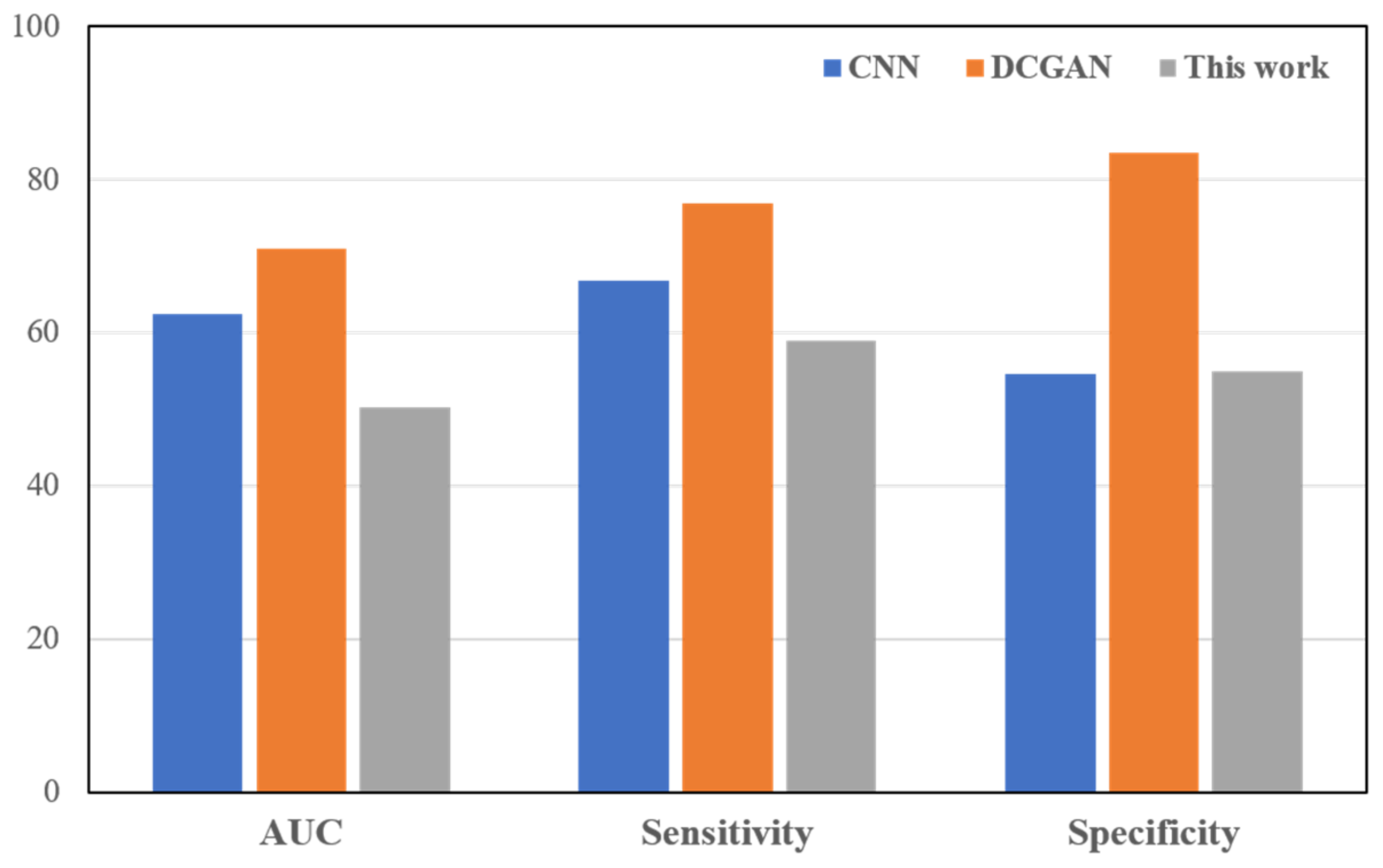
The proposed method in this paper addresses the shortcomings of DCGAN and improves upon the existing semi-supervised prediction model in terms of AUC, sensitivity, and specificity metrics. Additionally, for each evaluation metric, a corresponding analysis of the range of poor values was conducted, as shown in Figure 12. Comparing the proposed model in this study with the fully supervised training CNN [19] and the semi-supervised training DCGAN [28], the proposed model demonstrated lower ranges of poor values in most metrics. This indicates that the model has a smaller range of differences in detecting all patients.

Compared to the fully supervised prediction model, this method in the paper did not achieve optimal classification, but its results were comparable to the supervised prediction model CNN, and it achieved lower differences in detecting different patients. This research also has certain limitations and shortcomings. On the CHB-MIT dataset, the WGAN-GP-Bi-LSTM model demonstrated superior performance compared to existing semi-supervised epileptic seizure prediction methods. However, this method still needs to be further tested with more case data and validated using clinical data. Therefore, the generalizability of the proposed method needs to be further verified.

5. Conclusions and Further Works

In this study, an improved semi-supervised model for predicting epileptic seizures, WGAN-GP-Bi-LSTM, is proposed. This method uses Wasserstein Generative Adversarial Networks as the feature learning model, combining the Earth Mover’s distance and gradient penalty constraints for unsupervised training to train a high-order feature extractor. In the classifier part, a prediction model based on Bi-LSTM networks is constructed to improve epileptic seizure prediction performance based on high-frequency features of EEG signals. The method proposed in this study is semi-supervised, as it combines unsupervised training of adversarial network features with semi-supervised training of the classifier.

This model improves both the stability of the semi-supervised training model and the classifier and achieves good results in performance validation on the CHB-MIT dataset, with prediction AUC, sensitivity, and specificity metrics reaching 90.08%, 82.84%, and 85.97%, respectively. Comparison with previous related work demonstrates that this method is reliable, efficient, and suitable for real-time applications in epileptic seizure prediction. In the future, we will still require additional case data to conduct performance testing and consider how to balance data size and computation time. Additionally, using the VARFIMA model [42] to simulate the long-term memory characteristics of epileptic EEG signals in order to improve feature accuracy is the focus of our next research.