A Multi Brain Tumor Region Segmentation Model Based on 3D U-Net

Abstract

Accurate segmentation of different brain tumor regions from MR images is of great significance in the diagnosis and treatment of brain tumors. In this paper, an enhanced 3D U-Net model was proposed to address the shortcomings of 2D U-Net in the segmentation tasks of brain tumors. While retaining the U-shaped characteristics of the original U-Net network, an enhanced encoding module and decoding module were designed to increase the extraction and utilization of image features. Then, a hybrid loss function combining the binary cross-entropy loss function and dice similarity coefficient was adopted to speed up the model’s convergence and to achieve accurate and fast automatic segmentation. The model’s performance in the segmentation of brain tumor’s whole tumor region, tumor core region, and enhanced tumor region was studied. The results showed that the proposed 3D U-Net model can achieve better segmentation performance, especially for the tumor core region and enhanced tumor region tumor regions.

1. Introduction

Brain tumors are new organisms, which grow in the cranial cavity and can be divided into primary and secondary tumors. According to cancer statistics in recent years, the incidence of brain tumors accounts for about 1.5% of whole-body tumors, but the death rate is as high as 3% [1]. Glioma is one of the most common malignant tumors in the brain—a tumor, which originates from glial cells. There are two types of gliomas: high-grade gliomas (HGG) and low-grade gliomas (LGG) [2,3]. Magnetic resonance imaging (MRI) is one of the most commonly used tools in clinical medicine to examine the brain due to its non-invasive nature, which protects the body from ionizing radiation, and its superior soft tissue contrast [4]. The MRI scanner was adjusted with different parameters to obtain four modalities—T1, T2, T1ce, and Flair—as shown in Figure 1, which are multimodal brain MRI images of the same patient with the same acquisition device using different parameters. Due to the widespread use of MRI equipment in brain examinations, a large amount of brain MRI image data are generated in the clinic, and it is impossible for physicians to manually annotate and segment all images promptly. The tissue structure in brain tumor images varies from individual to individual, from stage to stage, and from device to device, and manual segmentation of brain tumor tissue relies on the physician’s personal experience. Therefore, the research focuses on how to segment brain tumors efficiently, precisely, and fully automatically [5].

Due to the outstanding effect of methods such as machine learning in image classification and segmentation, intelligent analysis of medical images based on artificial intelligence has been vigorously developed, and some effective semantic segmentation networks have been proposed, one after another, such as SegNet [6], DeepLab [7], U-Net [8], and so on. In particular, the 2D U-Net structure is now widely used in medical image segmentation. Pereria et al. [9] proposed an improved U-Net with novel feature reorganization and recalibration modules and segmented the tumor substructures in a cascade fashion. Jiang et al. [10] proposed a two-stage cascaded U-Net model, where the first stage uses a variant U-Net to obtain a rough segmentation result, and the second stage fuses the input with the first stage rough segmentation result and uses two decoders to improve the performance of the algorithm. Choi et al. [11] used two CNNs to process brain images for extracting global information and classifying voxels, respectively, after which the trained models were used for brain segmentation. Vaanathi et al. [12] proposed a multiple U-Net integrated network for brain tumor segmentation by extracting data in each of the three axes through three U-Nets, thus allowing multiple models to work in concert to achieve accurate segmentation of brain tumors. U-Net networks have been widely used in the field of brain tumor segmentation due to their powerful feature learning ability.

2. Related Work

In a two-dimensional U-Net network, two-dimensional convolutional kernels are used to acquire feature maps by sliding convolutional kernels from left to right and top to bottom on brain tumor MRI images [13]. MRI images are three-dimensional images, and even when multiple adjacent slices are used in a two-dimensional U-Net network, some of the stereoscopic information of the brain tumor can be preserved, but a significant amount of spatial information features will be lost. Therefore, considering a single MRI slice alone will have a certain number of false negatives in the segmentation results. A so-called false negative is an area, which is a tumor, and is predicted to be a non-tumor area. In contrast, the 3D convolutional neural network uses 3D convolutional kernels to add a front-to-back sliding direction in addition to left-to-right and top-to-bottom sliding on brain tumor MRI images to be able to extract brain tumor features, which can be complete. Mlynarski et al. [14] proposed a 2D–3D hybrid model to further improve the segmentation accuracy of tumors, but the network is complex and does not make sufficient use of tumor features. Colman et al. [15] proposed a 2D deep residual U-Net with 104 convolutional layers, replacing the convolutional blocks of each layer in the U-Net encoder with stacked “bottleneck” residual blocks, and it achieved good segmentation results in the 2D brain tumor segmentation task in 2020. Sun et al. [16] proposed a novel segmentation network, which can segment brain tumor subregions in MRI images more accurately by fusing multiscale features with complementary information in the encoder while employing an additive attention mechanism to reduce the semantic feature gap between the encoder and decoder during jump connection, but it still suffers from the relatively low segmentation accuracy of the tumor core and enhanced tumor compared to the whole tumor.

Tian et al. [17] designed a stacked residual block based on the original 3D U-Net network to address issues such as difficulty in training and slow convergence of the 3D U-Net network. While retaining more image features, it avoids the problem of deep network’s inability to converge. At the same time, it replaces the traditional dice loss function with a mixed loss function, which increases the contribution of brain tumor pixel regions to the total loss. The experimental results show that the accuracy of this algorithm has been improved to a certain extent. In 2017, Isensee et al. [18] were inspired by the U-Net network model and proposed a segmentation algorithm with a structure similar to the U-Net. They added a dropout layer between the convolutional layers, using 3 × 3 × 3 convolutional layers to replace the maximum pooling layer while using data augmentation technology to obtain more training data to prevent overfitting. Chen et al. [19] proposed an S3D-UNet structure for automatic segmentation of brain tumors. Adopting separable 3D convolutions instead of conventional convolutions solves the problems of high computational cost and high memory configuration in 3D convolutions. Not only does it reduce computational complexity, but it also fully utilizes the information of 3D MRI images. Experiments have shown that using separable 3D convolutions reduces computational costs, and the algorithm has achieved good results. Myronenko et al. [20] proposed a segmentation network for 3D MRI brain tumor images based on an encoding–decoding structure. A variational automatic encoder branch (VAE branch) was added at the end node of the encoder. Adding VAE branches can add additional guidance and normalization to the encoder output section, reconstruct the original input image, and optimize feature clustering results. This not only improves the performance of segmentation but also consistently achieves good training accuracy during any random initialization.

In this paper, an enhanced segmentation model of different brain tumor regions based on a 3D U-Net was proposed to address the above problems and to achieve better segmentation performance of different brain tumor regions. The main contributions of this paper are as follows:

(1)

An enhanced encoding module and decoding module were proposed to increase the extraction and utilization of image features.

(2)

The hybrid loss function combining the binary cross-entropy loss function and dice similarity coefficient was adopted to speed up the model’s convergence and to achieve accurate and fast automatic segmentation.

(3)

The model’s performance in the segmentation of brain tumor’s WT region, TC region, and ET region from MR images was studied. The results showed that the proposed 3D U-Net model can achieve better segmentation, especially for the TC and ET tumor regions.

In order to present the algorithm in this article more clearly, the advantages and disadvantages of the above algorithms and the algorithm in this article are summarized in

Table 1. Summary of advantages and disadvantages of brain tumor segmentation methods.

Model	Advantage	Disadvantage
Multi U-Net Integrated Network [12]	Three U-Nets work together with strong feature learning ability	Cross-validation resulted in overfitting of the network and incorrect prediction of the tumor core area
2D–3D [14]	Combining short distance 3D context and long distance 2D context, overcoming the limitations of specific selection of neural network architecture non-enhanced tumors	The network is relatively complex and does not fully utilize tumor features
DR-U-Net [15]	Replacing convolutional blocks with stacked residual blocks to enhance feature transfer	Class imbalance leads to a significant average DSC standard deviation between the validation and testing sets
Improving U-Net [18]	Injecting gradient signals deep into the network through deep supervision, extensively expanding data to prevent overfitting	Long network training time limits the number of architectural variants and data
VAE-encoder [20]	Adding VAE branches to provide additional guidance and standardization for the encoder output section	Cropping the image smaller in order to increase batch processing results in poor network feature extraction performance
Ours	Using enhanced encoding and decoding modules to improve the extraction and utilization of image features. The mixed loss function is used to accelerate the rate of convergence of the model	Blocking processing loses some information between blocks, resulting in poor segmentation performance for the whole tumor area

.

3. Methodology

MRI brain tumors are a three-dimensional data structure, and accurate 3D models are of great significance for doctors’ clinical diagnosis and treatment. In contrast, the segmentation algorithm based on a 2D network needs to slice it, and the sliced data are 2D data. The sliced data are 2D data, which makes the algorithm unable to learn the structural relationships between the layers of the data, resulting in insufficient learning of the network model. Moreover, the stacking of 2D slice segmentation results alone at a later stage may result in the formation of jagged or faulty phenomena, missing the spatial feature expression of the tumor. Therefore, it is very necessary to use 3D full convolutional neural network to solve such problems.

The structure of the enhanced brain tumor segmentation model based on the 3D U-Net is shown in Figure 2. The encoding path on the left side is mainly used for tumor feature extraction of the input MRI images and controls the feature map size of the output layer. The decoding path on the right restores the size of the feature map through skip connections and deconvolution, i.e., the feature map is reduced to the same size as the input image and achieves pixel-level point-to-point segmentation. The four input channels correspond to the images of the four MRI modalities. The three output channels correspond to the three brain tumor regions to be segmented, namely the whole tumor (WT) region, tumor core (TC) region, and enhanced tumor (ET) region.

3.1. Encoding Module

The schematic diagram of the encoding module is shown in Figure 3. A 3 × 3 × 3 convolution is added first for further feature extraction of the feature maps’ input to this module. Then, perform 1 × 1 × 1 convolution, 3 × 3 × 3 convolution, batch normalization (BN) [21], and rectified linear unit (ReLU) [22] operations three times in sequence. The 1 × 1 × 1 convolution has two main roles in the encoding module, one of which is to reduce the number of channels of the feature map to achieve the purpose of dimensionality reduction and reduce the computational complexity; the other is to integrate the information of each pixel point on different channels and add some non-linearity to the network. The 3 × 3 × 3 convolution is used to further extract image features.

The BN layer is added because it can perform a class normalization operation on the image data, so that the size scaling can be limited to a limited range, and the data that have significant differences can meet the roughly independent and identical distribution. This is reflected in the model by the increased learning speed during the training process. In addition, after normalization, the stability of the images is increased, and the influence of unchanged data is reduced because they are already approximately identically independently distributed; thus, the generalization ability of the model is further optimized.

The batch normalization layer requires the operations of mean, variance, normalization, and translation and scaling of the data input to the network, with the following procedure and equations:

$$B=\left\{x_{1\cdots m}\right\}$$

$${\mu }_B=\frac{1}{m}{\displaystyle {\sum }_{i=1}^m{x}_i}$$

(1)

$${\sigma }_B^2=\frac{1}{2}{{\displaystyle {\sum }_{i=1}^m(x_i-{\mu }_B)}}^2$$

(2)

$${\widehat{x}}_i=\frac{x_i-{\mu }_B}{\sqrt{{\sigma }_B^2+\epsilon }}$$

(3)

where ${\mu }_B$ is the mean value; ${\sigma }_B^2$ is the variance; ${\widehat{x}}_i$ is the normalization; $m$ is the sample size in the mini-batch; and $\epsilon$ is introduced to avoid a denominator of 0.

After these operations, the output of the encoding module is transmitted to the corresponding layer of the decoding module through skip connections, which increases the connection between low-level feature maps and high-level feature maps.

3.2. Decoding Module

The structure diagram of the decoding module is shown in Figure 4. It first performs a 3 × 3 × 3 up-convolution operation on the input feature map. Then, it is fused with the feature map from the corresponding encoding layer through skip connection, which increases the connection between the feature maps of the high and low levels. Finally, perform 1 × 1 × l convolution, 3 × 3 × 3 convolution, BN, and ReLU operations in sequence to reduce the dimensionality.

3.3. Loss Function

In this paper, a hybrid loss function combining cross-entropy loss and dice coefficient loss [23] is used. The cross-entropy loss can improve segmentation accuracy and ensure uniform background segmentation. The dice coefficient loss maximizes the dice coefficient to a value close to zero, resulting in a more rapid convergence of the model. The hybrid loss function in this paper combines the advantages of the two different loss functions, which can optimize the smooth gradient and the class imbalance.

The binary cross-entropy loss function is defined as

$$Los{s}_{BCE}=-\frac{1}{N}{\displaystyle \sum _{i=1}^{N}W\ast \left\{\left(T_n\log \left(P_n\right)\right)+\left(1-T_n\right)\ast \log \left(1-P_n\right)\right\}}$$

(4)

The dice loss function is defined as

$$Los{s}_{Dice}=1-\frac{2\left|X\cap Y\right|}{\left|X\right|+\left|Y\right|}$$

(5)

The hybrid loss function can be calculated through the equation

$$Los{s}_{Hybrid}=Los{s}_{BCE}+Los{s}_{Dice}$$

(6)

4. Experiments and Results

4.1. Dataset

Experimental data were obtained from the brain glioma public datasets BraTS2018 [24,25] and BraTS2019 [26,27] provided by the International Association for Medical Image Computing and Computer Aided Intervention (MICCAI). The training set in BraTS2019 has 285 cases (210 HGG patients and 75 LGG patients). An MR sequence has 155 images, each with a size of 240 × 240. Each case has four modalities (T1, T2, T1ce, Flair) and the corresponding standard segmentation label map (ground truth, GT). Compared with BraTS2019, BraTS2018 has 49 fewer HGGs and 1 fewer LGGs. In this paper, the extra 50 cases in BraTS2019 were used as the test set. The data in BraTs2018 are divided into a training set and a validation set in a 7:3 ratio, and each time the network is trained, they are randomly re-divided according to this ratio.

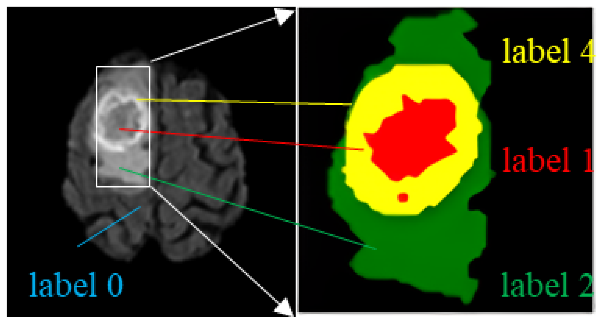
There are four label categories in the dataset: label 0 represents a healthy region; label 1 represents a region of necrotic and non-enhanced tumors; label 2 represents a peritumor edema region; and label 4 represents an enhanced tumor region. Brain tumors need to be segmented into three regions: the WT region, the TC region, and the ET region. WT includes the regions with labels 1, 2, and 4; TC includes labels 1 and 4; ET includes only label 4, as shown in

Table 2. Explanation of dataset labels.

Label Number	Label Meaning	Color Representation
0	a healthy region	/
1	a region of necrotic and non-enhanced tumors	region with red
2	a peritumor edema region	region with green
4	an enhanced tumor region	region with yellow

. An example of an MRI brain tumor image is shown in Figure 5, where each label is represented using a corresponding color: label 1 region with red, label 2 with green, and label 4 with yellow.

4.2. Evaluation Metrics

In this paper, the dice similarity coefficient (Dice), Precision, and Sensitivity are used as performance evaluation metrics, which can be expressed as follows:

$$Dice=\frac{2\left|P_1\cap T_1\right|}{\left|P_1\right|+\left|T_1\right|}=\frac{2TP}{FP+2TP+FN}$$

(7)

where TP denotes the number of positive classes correctly detected; FN denotes the number of positive classes mistaken for negative classes; and FP denotes the number of negative class samples mistaken for positive class samples.

The dice similarity coefficient indicates the overlap rate of the algorithm segmentation results with the real labels. When the value of the dice is 0, the segmentation result is the worst, which means that all the pixel points segmented by the algorithm do not overlap with all the pixel points of the standard segmentation label; when the value of the dice is 1, it means that all the pixel points of the actual segmentation result overlap with the corresponding position of the real label, and the segmentation result is the best at this time.

Precision is defined as

$$Precision=\frac{\left|P_1\cap T_1\right|}{\left|P_1\right|}=\frac{TP}{TP+FP}$$

(8)

Precision indicates that the positive predictive value is similar to the true positive rate, reflecting the accuracy of the actual segmentation results. A higher precision value means that more pixels are correctly classified in the actual segmentation result.

Sensitivity is defined as

$$Sensitivity=\frac{\left|P_1\cap T_1\right|}{\left|T_1\right|}=\frac{TP}{TP+FN}$$

(9)

Sensitivity indicates the ratio of focal areas correctly predicted by the model to the true labeled focal areas and measures the sensitivity of the model to the focal areas.

4.3. Pre-Processing

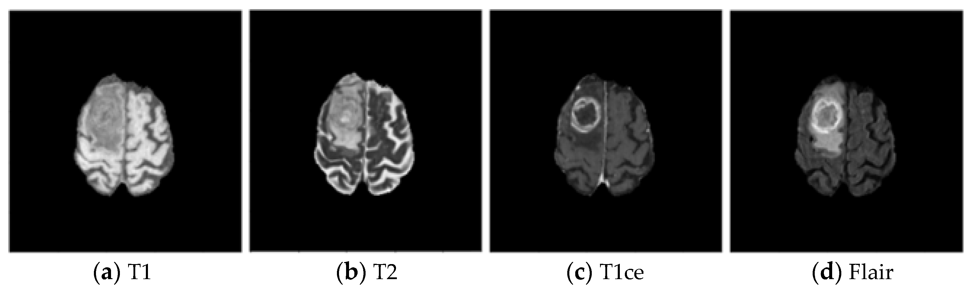
BraTS2018 and BraTS2019 use four sequences of MR images—T1, T2, T1ce, and Flair—which have different contrasts. Therefore, the z-score method is used to standardize each modal image separately, subtracting the mean from the image and dividing it by the standard deviation to eliminate the impact of different contrasts [28]. In an MRI image, the gray area represents the brain region, while the black area represents the background. The background has a large proportion in the entire image and is not helpful for segmentation. Therefore, it is necessary to remove the background information around the brain region. Meanwhile, cropping makes the network a little smaller and improves the performance of the network. Since the whole 3D image occupies too much RAM and affects the input of the network, this experiment requires chunking of the 3D MRI images. To chunk evenly, five black slices are added to the original sequence, that is, four modal images and the corresponding mask (155, 240, 240). The chosen chunk size is 32, 160, 160, i.e., five chunks with size of 32, 160, 160 are divided from the axial direction, and the resolution of the chunks is set to an even number to make them integer divisible when they are down-sampled through the pooling layer.

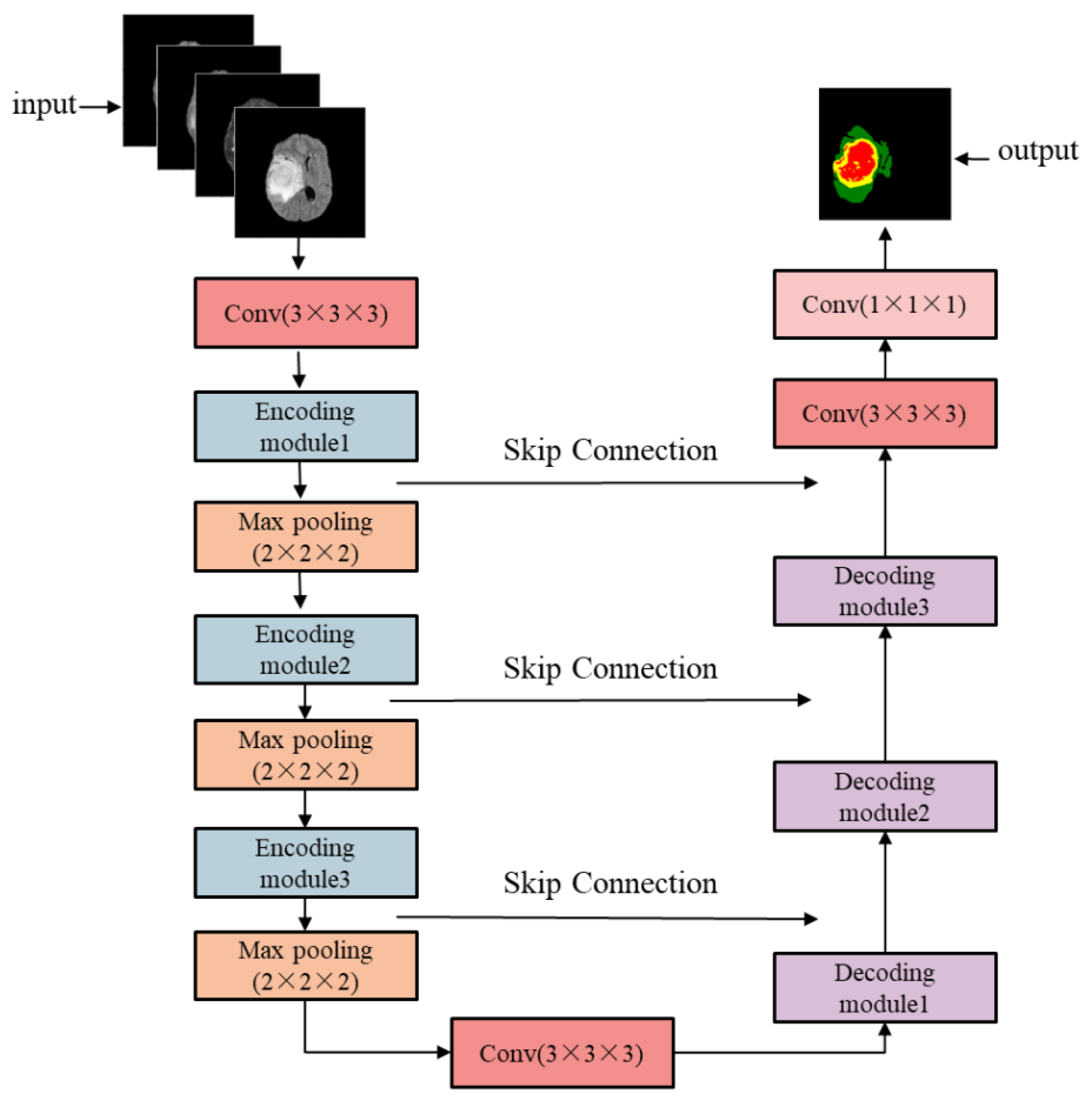
4.4. Results and Discussion

All experiments in this paper were conducted in the same training environment configuration: AMD 5950X, CPU 64GB RAM, and NVIDIA GeForce RTX3090 24G GPU. PyTorch1.12 framework and Anaconda Python3.7 interpreter built the network framework. The weight decay is 1 × 10⁻⁴; the total epoch is 100 times; the initial learning rate is 3 × 10⁻⁴; the batch size is 4; and the activation function is Softmax.

To evaluate the segmentation performance of the proposed model, comparative experiments were conducted in three aspects.

Table 3. Comparison of dice similarity coefficient with ten other models.

Model	WT Dice	TC Dice	ET Dice
U-Net	0.838	0.821	0.768
U-Net++	0.842	0.826	0.774
PA-Net	0.801	0.681	0.718
S3D-UNet [19]	0.880	0.756	0.659
VAE-encoder [20]	0.882	0.814	0.733
DANet [29]	0.842	0.853	0.797
ResUnet [30]	0.843	0.861	0.787
AttUNet [31]	0.849	0.866	0.789
MA-UNet [32]	0.738	0.743	0.577
SAU-Net [33]	0.815	0.843	0.712
ANU-Net [34]	0.811	0.866	0.733
Attention-UNet [35]	0.843	0.858	0.685
Ours	0.778	0.875	0.903

gives the comparison of the dice similarity coefficient of the proposed model with the other ten models in the extraction of WT, TC, and ET. From Table 3, it can be concluded that our model significantly improved overall accuracy compared to the 2D segmentation networks, especially in the ET area. It also handles the details of the TC area well. The dice similarity coefficient of WT reaches 0.778; TC dice reaches 0.875, which is about 0.054 higher than that of the 2D U-Net; ET dice reaches 0.903, which is about 0.137 higher than that of the 2D U-Net.

Table 4. Comparison of sensitivity with ten other models.

Model	WT Sensitivity	TC Sensitivity	ET Sensitivity
U-Net	0.868	0.917	0.801
U-Net++	0.868	0.912	0.827
PA-Net	0.800	0.675	0.759
S3D-UNet [19]	0.886	0.737	0.704
VAE-encoder [20]	0.891	0.815	0.745
DANet [29]	0.885	0.915	0.839
ResUnet [30]	0.875	0.895	0.843
AttUNet [31]	0.878	0.918	0.848
MA-UNet [32]	0.795	0.815	0.653
SAU-Net [33]	0.788	0.858	0.758
ANU-Net [34]	0.858	0.842	0.763
Attention-UNet [35]	0.852	0.893	0.808
Ours	0.906	0.926	0.946

gives the sensitivity comparison of the proposed model with the other ten models in the extraction of WT, TC, and ET. As shown in Table 4, the sensitivity of WT, TC, and ET reaches 0.906, 0.926, and 0.946, respectively, which represents an improvement of 3.8%, 0.9%, and 6.5% compared to the 2D U-Net. This shows that the 3D U-Net model designed in this paper can better handle the segmentation of different tumor regions.

Table 5. Comparison of precision with ten other models.

Model	WT Precision	TC Precision	ET Precision
U-Net	0.856	0.853	0.774
U-Net++	0.866	0.850	0.791
PA-Net	0.792	0.695	0.681
S3D-UNet [19]	0.891	0.852	0.635
VAE-encoder [20]	0.895	0.854	0.758
DANet [29]	0.859	0.893	0.781
ResUnet [30]	0.871	0.891	0.787
AttUNet [31]	0.888	0.892	0.786
MA-UNet [32]	0.732	0.799	0.574
SAU-Net [33]	0.755	0.783	0.678
ANU-Net [34]	0.703	0.795	0.704
Attention-UNet [35]	0.788	0.808	0.655
Ours	0.801	0.895	0.946

gives the precision comparison of the proposed model with the other ten models in the extraction of WT, TC, and ET. As shown in Table 5, the model in this paper outperforms other models in terms of TC precision and ET precision, reaching 0.895 and 0.946, respectively. However, WT precision is relatively low, only reaching 0.801.

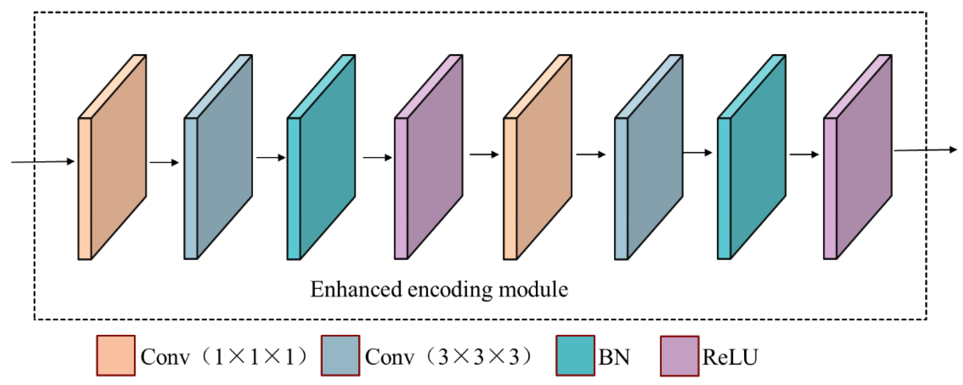
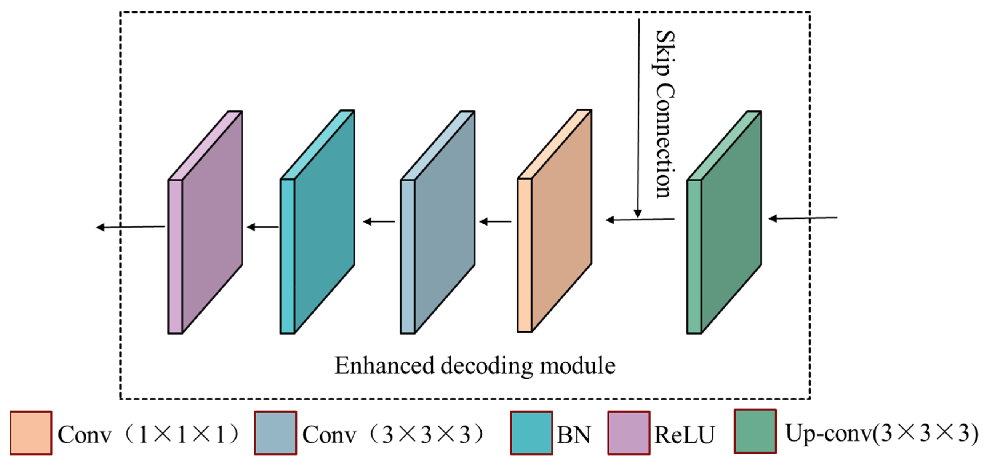
The binary cross-entropy loss function can optimize the network in the process of network training, effectively solve the problem of vanishing gradient in the network, and make the network run stably. However, when faced with images with class imbalance problems, the loss function will exhibit bias toward samples with many classes, thus affecting the optimization direction of the network. The dice similar loss function can guide the learning of network parameters and make the prediction result close to the real value.

In this paper, experiments are conducted to verify whether adding the dice similar loss function to the binary cross-entropy loss function can improve the performance of glioma segmentation. The experimental results are shown in

Table 6. Segmentation evaluation results of different loss functions.

Model Structure	Dice			Sensitivity			Precision
	WT	TC	ET	WT	TC	ET	WT	TC	ET
Model+BCE	0.871	0.819	0.775	0.891	0.825	0.789	0.885	0.892	0.767
Model+BCE+Dice	0.778	0.875	0.903	0.906	0.926	0.946	0.801	0.895	0.946

.

It can be seen from Table 5 that the mixed loss function composed of binary cross- entropy loss function and dice similarity coefficient can alleviate the class imbalance problem in brain glioma image segmentation to a certain extent and obtain good network segmentation results.

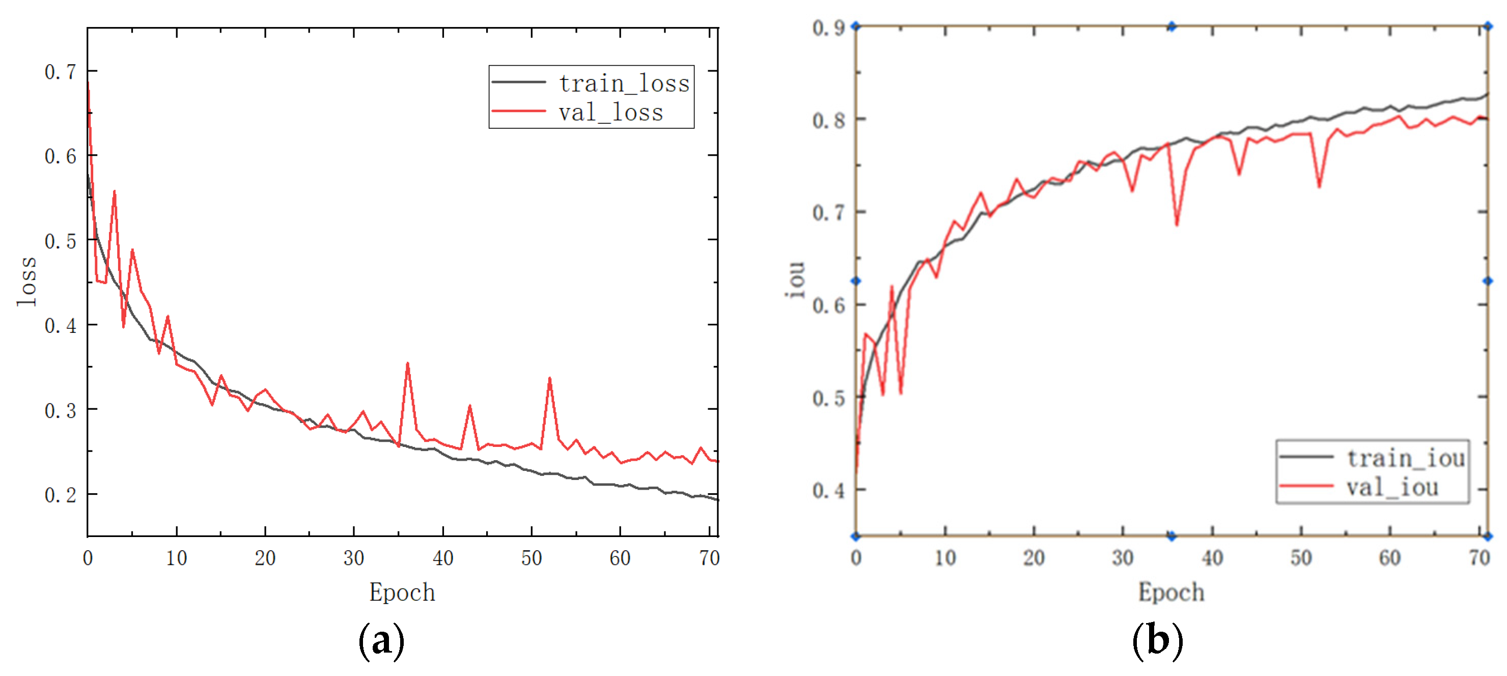
To verify the advantages of this paper’s model more intuitively, the change curves of loss and Iou with the number of epochs in the training and validation sets during the training process are shown in Figure 6, which can intuitively show the superiority of this paper’s algorithm.

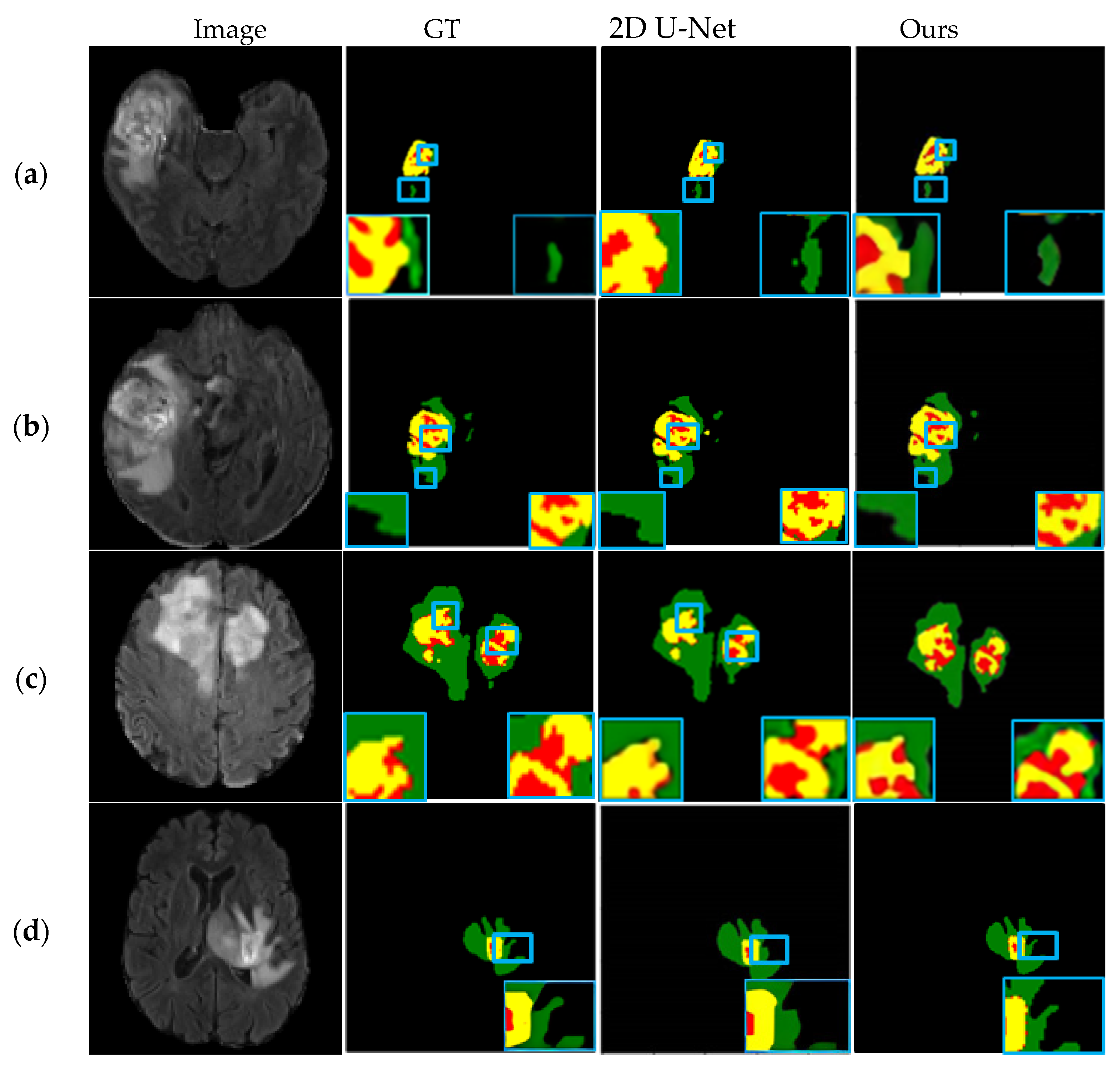
The extraction effects of different tumor regions are shown in Figure 7. The first column depicts the original Flair MR images of four different cases. Columns 2–4 are their corresponding segmentation results of the GT, 2D U-Net, and 3D U-Net models in this paper.

As can be seen in Figure 7a, the overall segmentation effect of the network in this paper is better, and the boundaries of different tumor regions can be segmented more accurately, especially the tumor core area, and the segmentation results are similar to GT. As can be seen in Figure 7b,c, the tumor enhancement region and the core region are segmented more accurately, and the contour boundary is clearer, and the brain tumor segmentation results prove that the algorithm in this paper has better segmentation performance. In Figure 7d, the location of the tumor is determined, but the boundary segmentation of the edema area around the tumor is relatively rough, and the segmentation effect of the whole tumor area is not very satisfactory, and the network will continue to be improved subsequently.

5. Conclusions and Future Work

In this paper, an enhanced 3D U-Net segmentation model was proposed to address the shortcomings of 2D networks in handling brain tumor segmentation tasks. While retaining the original U-shaped network framework, the structure of the encoder and decoder is recompiled, i.e., the same convolution is used in the coder–decoder module instead of the valid convolution used in the original network to enhance the re-utilization of the feature map. The network model is optimized by adding a 1 × 1 × 1 convolution to reduce the dimensionality and the computation of the network while finding the optimal hybrid loss function to improve the learning ability of the network model and further improve the segmentation accuracy of the lesion region. The results showed that the model’s segmentation performance of both TC regions and ET regions was superior to those of other 2D U-Net models, and its sensitivity reached 90.6%, 92.6%, and 94.6% for the WT region, the TC region, and the ET region, respectively.

The algorithm designed in this article has good segmentation performance for the tumor core area and tumor enhancement area, but there are shortcomings in the dice index for the entire tumor area. In the future, further improvements are needed to the network structure, such as adding attention mechanisms to improve the segmentation of the entire tumor area. This article uses a skip connection method to concatenate the extracted feature maps from the encoding module directly to the corresponding layer of the decoding module. However, the extracted low-level features have redundant information. The use of attention mechanism can effectively suppress activation in irrelevant regions and reduce redundant parts of skip connections. At the same time, the network model should be optimized; the encoding and decoding modules should be simplified; and the network training speed should be improved.

References

1. Liang, F.X.; Yang, F.; Lu, L.Y. Review of Brain Tumor Segmentation Methods Based on Convolutional Neural Networks. Comput. Eng. Appl. 2021, 57, 34–43. [Google Scholar]
2. Menze, B.H.; Jakab, A.; Bauer, S. The multimodal brain tumor image segmentation benchmark (BraTS). IEEE Trans. Med. Imaging 2015, 34, 1993–2024. [Google Scholar] [CrossRef] [PubMed]
3. Masood, M.; Nazir, T.; Nawaz, M.; Mehmood, A.; Rashid, J.; Kwon, H.-Y.; Mahmood, T.; Hussain, A. A Novel Deep Learning Method for Recognition and Classification of Brain Tumors from MRI Images. Diagnostics 2021, 11, 744. [Google Scholar] [CrossRef]
4. Hao, L.; Guanhua, W.; Qiang, Z. Optimization of Dice Loss Function for 3D Brain Tumor Segmentation. China Med. Devices 2019, 34, 20–23, 31. [Google Scholar]
5. Mishra, P.; Garg, A.; Gupta, D. Review on brain tumor segmentation: Hard and soft computing approaches. In Proceedings of the International Conference on Image Processing and Capsule Networks, ICIPCN 2020, Bangkok, Thailand, 6–7 May 2020; pp. 190–200. [Google Scholar]
6. Badrinarayanan, V.; Kendall, A.; Cipolla, R. SegNet: A Deep Convolutional Encoder-Decoder Architecture for Image Segmentation. IEEE Trans. Pattern Anal. Mach. Intell. 2017, 39, 2481–2495. [Google Scholar] [CrossRef]
7. Niu, Z.; Liu, W.; Zhao, J.; Jiang, G. DeepLab-Based Spatial Feature Extraction for Hyperspectral Image Classification. IEEE Geosci. Remote Sens. Lett. 2019, 16, 251–255. [Google Scholar] [CrossRef]
8. Long, J.; Shelhamer, E.; Darrell, T. Fully Convolutional Networks for Semantic Segmentation. IEEE Trans. Pattern Anal. Mach. Intell. 2015, 39, 640–651. [Google Scholar]
9. Pereira, S.; Pinto, A.; Alves, V. Brain Tumor Segmentation Using Convolutional Neural Networks in MRI Images. IEEE Trans. Med. Imaging 2016, 35, 1240–1251. [Google Scholar] [CrossRef]
10. Jiang, Z.; Ding, C.; Liu, M. Two-Stage Cascaded U-Net: 1st Place Solution to BraTS Challenge 2019 Segmentation Task; Springer: Cham, Switzerland, 2020. [Google Scholar]
11. Choi, H.; Jin, K.H. Fast and robust segmentation of the striatum using deep convolutional neural networks. J. Neurosci. Methods 2016, 274, 146–153. [Google Scholar] [CrossRef]
12. Sundaresan, V.; Griffanti, L.; Jenkinson, M. Brain Tumor Segmentation Using a Tri-Planar Ensemble of U-Nets; Springer: Cham, Switzerland, 2021. [Google Scholar]
13. Guoxiu, J. An introduction to convolutional neural networks. Heilongjiang Sci. Technol. Inf. 2017, 43–47. [Google Scholar]
14. Mlynarski, P.; Delingette, H.; Criminisi, A. 3D Convolutional Neural Networks for Tumor Segmentation using Long-range 2D Context. Comput. Med. Imaging Graph. 2018, 73, 60–72. [Google Scholar] [CrossRef] [PubMed]
15. Colman, J.; Zhang, L.; Duan, W.; Ye, X. DR-Unet104 for Multimodal MRI brain tumor segmentation. Lect. Notes Comput. Sci. 2020, 12659, 410–419. [Google Scholar]
16. Sun, J.K.; Zhang, R.; Guo, L.J.; Wang, J. Multi-scale feature fusion and additive attention guide brain tumor MR image segmentation. J. Image Graph. 2023, 28, 1157–1172. [Google Scholar]
17. Xuezhi, T.; Lianying, Z. Design of tumor segmentation method based on 3D U-Net network. Comput. Digit. Eng. 2022, 50, 405–409, 418. [Google Scholar] [CrossRef]
18. Isensee, F.; Kickingereder, P.; Wick, W.; Bendszus, M.; Maier-Hein, K.H. Brain Tumor Segmentation and Radiomics Survival Prediction: Contribution to the BRATS 2017 Challenge. Int. MICCAI Brainlesion Workshop 2017, 10670, 287–297. [Google Scholar]
19. Chen, W.; Liu, B.; Peng, S.; Sun, J.; Qiao, X. S3D-UNet: Separable 3D U-Net for brain tumor segmentation. In Glioma, Multiple Sclerosis, Stroke and Traumatic Brain Injuries, Proceedings of the 4th International Workshop, BrainLes 2018, Granada, Spain, 16 September 2018; Springer International Publishing: Cham, Switzerland, 2019; pp. 358–368. [Google Scholar]
20. Myroneko, A. 3D MRI Brain Tumor Segmentation Using Autoencoder Regularization; Springer International Publishing: Cham, Switzerland, 2019; Volume 11384, pp. 311–320. [Google Scholar]
21. Li, Y.; Wang, N.; Shi, J.; Hou, X.; Liu, J. Adaptive Batch Normalization for practical domain adaptation. Pattern Recognit. 2018, 80, 109–117. [Google Scholar] [CrossRef]
22. Petersen, P.; Voigtlaender, F. Optimal approximation of piecewise smooth functions using deep ReLU neural networks. Neural Netw. 2018, 108, 296–330. [Google Scholar] [CrossRef]
23. Thada, V.; Jaglan, D.V. Comparison of Jaccard, Dice, Cosine Similarity Coefficient To Find Best Fitness Value for Web Retrieved Documents Using Genetic Algorithm. Int. J. Innov. Eng. Technol. 2013, 2, 202–205. [Google Scholar]
24. Arora, A.; Jayal, A.; Gupta, M.; Mittal, P.; Satapathy, S.C. Brain Tumor Segmentation of MRI Images Using Processed Image Driven U-Net Architectur. Computers 2021, 10, 139. [Google Scholar] [CrossRef]
25. Bakas, S.; Akbari, H.; Sotiras, A. Advancing The Cancer Genome Atlas glioma MRI collections with expert segmentation labels and radiomic features. Sci. Data 2017, 4, 170117. [Google Scholar] [CrossRef]
26. Hu, K.; Gan, Q.; Zhang, Y. Brain Tumor Segmentation Using Multi-Cascaded Convolutional Neural Networks and Conditional Random Field. IEEE Access 2019, 7, 92615–92629. [Google Scholar] [CrossRef]
27. Saeed, M.U.; Ali, G.; Bin, W.; Almotiri, S.H.; AlGhamdi, M.A.; Nagra, A.A.; Masood, K.; Amin, R.U. RMU-Net: A Novel Residual Mobile U-Net Model for Brain Tumor Segmentation from MR Images. Electronics 2021, 10, 1962. [Google Scholar] [CrossRef]
28. Fu, S.; Wang, C.; Luo, J.; Liu, X. Segmentation Method of Brain Tumor MR Image Based on Improved U—Net Model. J. China West Norm. Univ. (Nat. Sci.) 2021, 42, 202–208. [Google Scholar]
29. Fu, J.; Liu, J.; Tian, H. Dual Attention Network for Scene Segmentation. In Proceedings of the 2019 IEEE/CVF Conference on Computer Vision and Pattern Recognition (CVPR), Long Beach, CA, USA, 15–20 June 2020. [Google Scholar]
30. Alom, M.Z.; Yakopcic, C.; Hasan, M. Recurrent residual U-Net for medical image segmentation. J. Med. Imaging 2019, 6, 014006. [Google Scholar] [CrossRef] [PubMed]
31. Schlemper, J.; Oktay, O.; Schaap, M.; Heinrich, M.; Kainz, B.; Glocker, B.; Rueckert, D. Attention gated networks: Learning to leverage salient regions in medical images. Med. Image Anal. 2019, 53, 197–207. [Google Scholar] [CrossRef]
32. Cai, Y.; Wang, Y. MA-Unet: An improved version of Unet based on multi-scale and attention mechanism for medical image segmentation. arXiv 2020, arXiv:2012.10952. [Google Scholar]
33. Zhang, Y.; Yuan, L.; Wang, Y.; Zhang, J. SAU-Net: Efficient 3D Spine MRI Segmentation Using Inter-Slice Attention. Med. Imaging Deep Learn. PMLR 2020, 121, 903–913. [Google Scholar]
34. Li, C.; Tan, Y.; Chen, W. ANU-Net: Attention-based Nested U-Net to exploit full resolution features for medical image segmentation. Comput. Graph. 2020, 90, 11–20. [Google Scholar] [CrossRef]
35. Oktay, O.; Schlemper, J.; Folgoc, L.L. Attention U-Net: Learning Where to Look for the Pancreas. arXiv 2018, arXiv:1804.03999. [Google Scholar]
Figure 1. Brain tumor images in different modes.
Applsci 13 09282 g001
Figure 2. Overall structure of the enhanced brain tumor extraction model.
Applsci 13 09282 g002
Figure 3. The structure diagram of the enhanced encoding module.
Applsci 13 09282 g003
Figure 4. The structure diagram of the enhanced decoding module.
Applsci 13 09282 g004
Figure 5. Different labels and tumor regions in MR images.
Applsci 13 09282 g005
Figure 6. Curves of loss and Iou for the training and validation sets, where (a) is a plot of the variation of loss with epoch and (b) is a plot of the variation of Iou with epoch.
Applsci 13 09282 g006
Figure 7. Segmentation results of four different cases: (a) Case 1; (b) Case 2; (c) Case 3; (d) Case 4.
Applsci 13 09282 g007