Article

Impact of Traditional and Embedded Image Denoising on CNN-Based Deep Learning

Institute of Innovation Science and Sustainability, Federation University Australia, Ballarat 3350, Australia
*
Author to whom correspondence should be addressed.
Appl. Sci. 2023, 13(20), 11560; https://doi.org/10.3390/app132011560
Submission received: 4 September 2023 / Revised: 18 October 2023 / Accepted: 20 October 2023 / Published: 22 October 2023
(This article belongs to the Special Issue IoT in Smart Cities and Homes)

Abstract

:
In digital image processing, filtering noise is an important step for reconstructing a high-quality image for further processing such as object segmentation, object detection, and object recognition. Various image-denoising approaches, including median, Gaussian, and bilateral filters, are available in the literature. Since convolutional neural networks (CNN) are able to directly learn complex patterns and features from data, they have become a popular choice for image-denoising tasks. As a result of their ability to learn and adapt to various denoising scenarios, CNNs are powerful tools for image denoising. Some deep learning techniques such as CNN incorporate denoising strategies directly into the CNN model layers. A primary limitation of these methods is their necessity to resize images to a consistent size. This resizing can result in a loss of vital image details, which might compromise CNN’s effectiveness. Because of this issue, we utilize a traditional denoising method as a preliminary step for noise reduction before applying CNN. To our knowledge, a comparative performance study of CNN using traditional and embedded denoising against a baseline approach (without denoising) is yet to be performed. To analyze the impact of denoising on the CNN performance, in this paper, firstly, we filter the noise from the images using traditional means of denoising method before their use in the CNN model. Secondly, we embed a denoising layer in the CNN model. To validate the performance of image denoising, we performed extensive experiments for both traffic sign and object recognition datasets. To decide whether denoising will be adopted and to decide on the type of filter to be used, we also present an approach exploiting the peak-signal-to-noise-ratio (PSNRs) distribution of images. Both CNN accuracy and PSNRs distribution are used to evaluate the effectiveness of the denoising approaches. As expected, the results vary with the type of filter, impact, and dataset used in both traditional and embedded denoising approaches. However, traditional denoising shows better accuracy, while embedded denoising shows lower computational time for most of the cases. Overall, this comparative study gives insights into whether denoising will be adopted in various CNN-based image analyses, including autonomous driving, animal detection, and facial recognition.

1. Introduction

In the transportation, agriculture, and defence sectors, weather phenomena can have various negative consequences [1,2,3,4]. In these sectors, images are captured in the outdoor environment. When images are acquired, compressed, and transmitted, noise is inherently introduced by the environment, camera, and other factors, resulting in distortion and loss of information. With the presence of noise, image processing tasks, such as object recognition and segmentation, edge detection, and feature extraction are adversely affected [5]. This is because the contrast, edges, textures, object details, and quality of a noisy image are impacted, lowering the post-processing algorithm’s performance [6]. Therefore, image denoising plays an important role in modern image processing systems.
Image denoising is used to remove noise from a noisy image, to restore the true image. As noise, edge, and texture are high-frequency components; it is difficult to distinguish them in the denoising process, and some details may be lost as a result. In general, recovering meaningful information from noisy images to obtain high-quality images has become an increasingly important problem [7].
Different kinds of widely adopted image-denoising filters are used to remove noise from the images impacted by various environmental and camera parameters [8]. The widely used image noise denoising techniques are median [9], Gaussian [10], and bilateral filters [11,12]. Various traditional approaches exist for image noise removal where images are denoised as a preprocessing step. For example, for object detection, firstly, images are denoised using a depth filter. Secondly, objects are recognized using the convolutional neural network (CNN) [13]. Another example is [14], where images are pre-processed with Gaussian blur. The simulation of a self-driving car has been carried out, which can learn to drive autonomously without manual intervention of human beings using deep CNN. A few other approaches of deep learning such as CNN having embedded image denoising are available in the current literature. Examples of these techniques are [15,16,17]. Images collected from different sources may have different sizes. Since the size of the convolution kernel of CNNs is fixed in CNN-based deep learning techniques, the resizing of images while denoising is required, which leads to the loss of information in the images. The image resizing process may involve both downscaling and upscaling images. While downscaling results in image information being lost, there is the possibility of the addition of redundant information in images during upscaling as well. To our knowledge, no comparative performance analysis study on the performance of CNNs for traditional and embedded image denoising exists in the current literature. Besides the performance study presented in this paper, the results show that denoising cannot produce superior recognition accuracy for some impacts such as shadow and darkness compared with “without denoising”. This insight raises the question of whether we should adopt denoising for the dataset affected by a particular impact. To address this research question, we calculate the distribution of the PSNRs of all images of a dataset before and after denoising. We devise two principles that help to decide whether the overall quality of images has been improved after denoising.

Motivation and Contributions of Research Work

People are working to embed filtering techniques in machine learning models for visual analysis, especially deep learning. To our knowledge, how this embedded technique works compared to its traditional denoising counterpart is yet to be performed. This research gap motivates us to perform a comparative study between traditional and embedded denoising. We choose to analyze the performance of CNN for IoT image recognition applications using different types of environmental impacts such as rain, shadow, snow, darkness, and exposure. Camera impacts include lens blur and lens dirtiness. As expected, denoising does not work for all types of impacts because all denoising techniques consider the basic conceptual models for image filtering that are developed exploiting the characteristics of general noises such as white Gaussian noise and salt and pepper noise. These filtering techniques are not generic enough to encode the characteristics of all types of impacts, raising the question of whether we should apply a denoising approach for a particular impact. If the use of the denoising approach is decided, what type of denoising approach will be adopted? To address this research issue, this study also proposes a conceptual approach that will help in deciding whether and which type of denoising approach should be applied for a particular impact in a recognition dataset. The major contributions of the paper are as follows:
  • We filter image noise from training and test data sets using traditional methods of filtering noise such as median filter and Gaussian filter.
  • We embed a layer for image denoising in the CNN model. Then, we compare the traffic sign and general object recognition accuracy and processing time for the CNN algorithm with the traditional approach of denoising and embedded denoising against a baseline approach called without denoising.
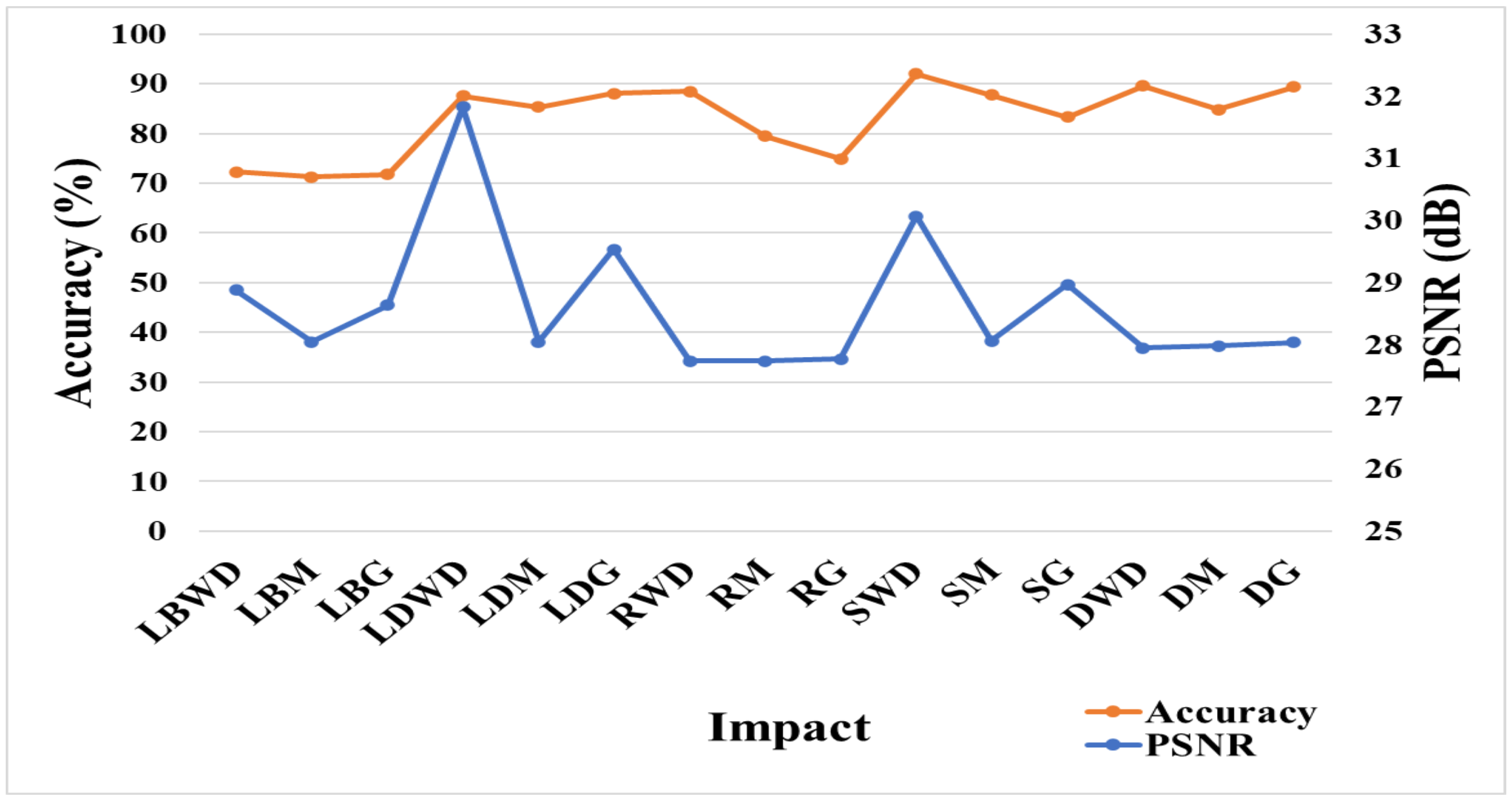
  • For the detection accuracy and computational time performance, we use challenging unreal and real environments for traffic sign recognition (CURE-TSR) [18] and challenging unreal and real environments for object recognition (CURE-OR) [19] datasets. We use environmental impacts such as rain, shadow, darkness, and snow. For camera impacts, we cover lens blur and lens dirtiness from both CURE-TSR and CURE-OR datasets. We utilize impacts such as contrast, salt and pepper noise, overexposure, and underexposure, from the CURE-OR dataset. The recognition accuracy of CNN for the traditional denoising approach shows superior performance to that when image denoising is embedded in CNN.
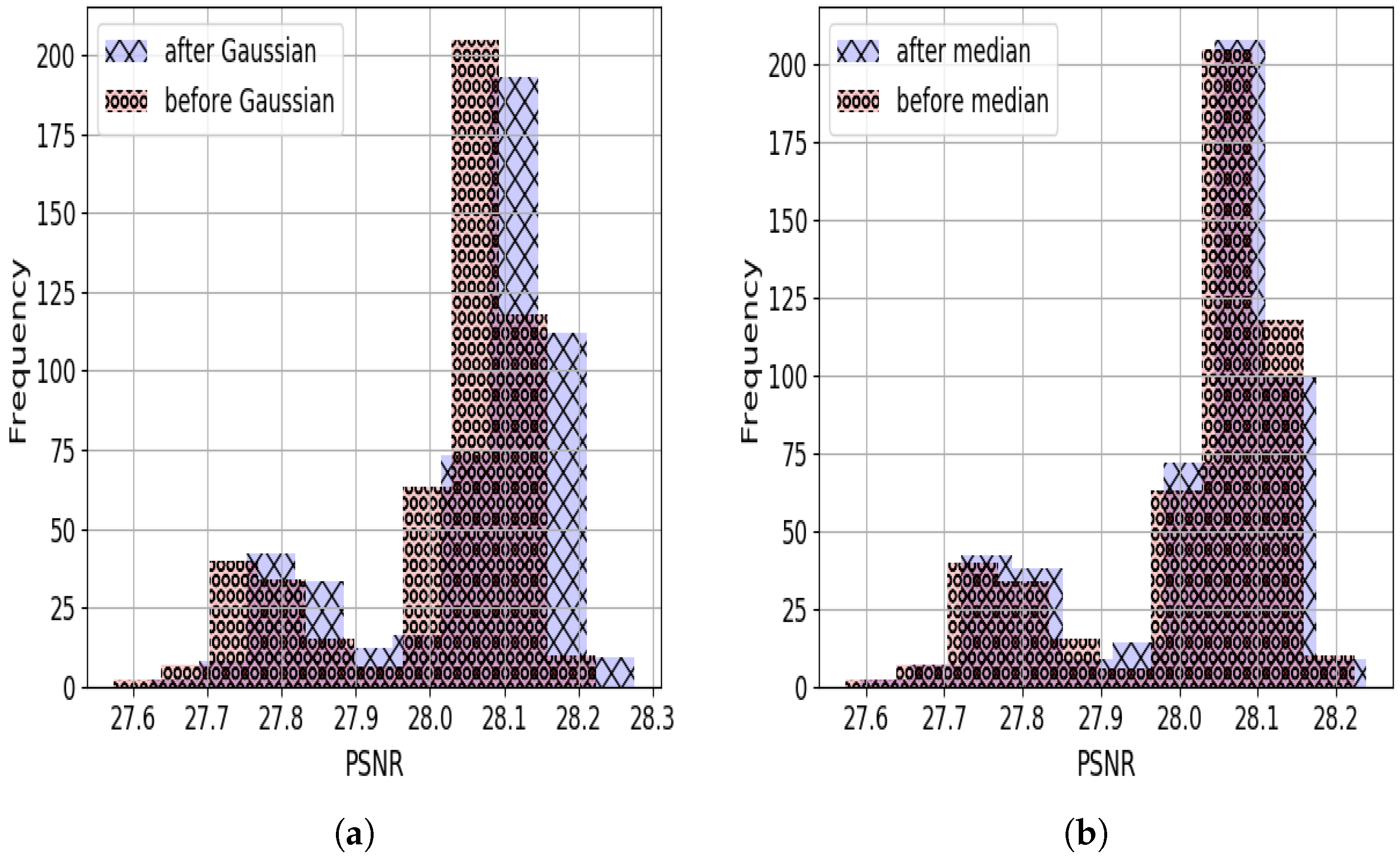
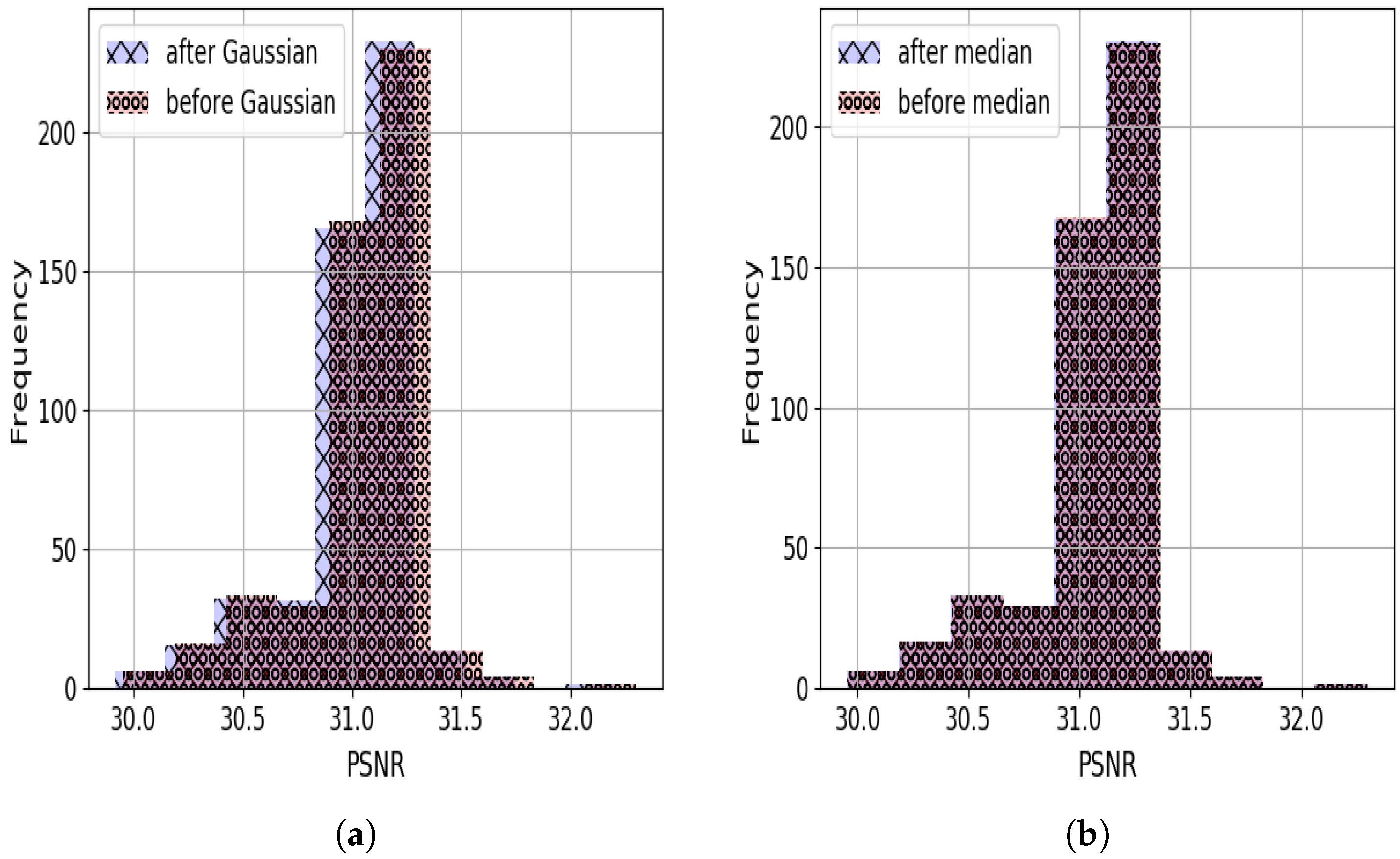
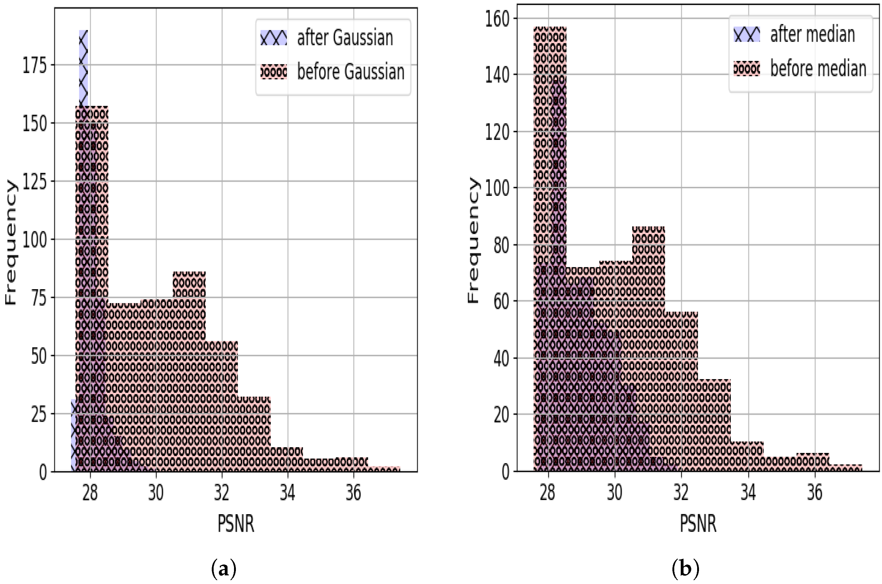
  • To decide whether denoising would be adopted, we calculate the distribution (histogram) of PSNRs of the images of the dataset affected by impacts before and after denoising. Through PSNR histograms, we assess whether the quality of images has been improved based on our developed two principles. The histograms were produced using the two data sets for all impact types mentioned in Contribution 3 for the median and Gaussian filters. When the overall quality of images is improved after denoising, these histograms support the adoption of filtering for CNN-based image recognition.
The rest of this paper is organized as follows. Related works are mentioned in Section 2. Section 3 elaborates on our comparative performance study and an approach to decide whether denoising will be adopted. Section 4 gives comprehensive experimental results with the comparative approach. Conclusions are drawn in Section 5.

2. Literature Review

Image denoising is extensively investigated in various contexts such as computer vision [20], digital photography, medical image analysis, remote sensing, surveillance, and digital entertainment [21]. Since this research project focuses on the performance study of deep learning (CNN) for traditional and embedded denoising, the following sections review the literature associated with them.

2.1. Image Denoising Techniques

Widely used image-denoising filters are median, Gaussian, and bilateral filters [22]. Median filters are widely considered to be the most effective way to eliminate salt and pepper noises. Low-density impulse noise can be effectively eliminated by it [23]. Using the median filter, noise is removed from an image, and edge detection is improved. A positive odd integer is used for the kernel size [24]. Another filter is the Gaussian filter, which we use for image denoising. Gaussian filters smooth images more effectively [25]. It is based on Gaussian distribution. The probability density function (P(x)) of Gaussian distribution is represented by Equation (1).
P ( x ) = 1 2 n σ 2 e ( x μ ) 2 / ( 2 σ 2 )
Here, x is a grey level intensity of a pixel belonging to a window in an image. μ is the mean pixel intensity value of all pixels within that window, and σ is the standard deviation [26]. The amount of smoothing of the Gaussian is determined by standard deviation σ . The Gaussian filter takes the neighborhood around the pixel and finds its Gaussian weighted average. A Gaussian filter is based solely on space, that is, nearby pixels are taken into account during filtering. No consideration is given to pixels with nearly the same intensity. The algorithm does not take into account whether a pixel is an edge pixel or not. The edges are also blurred in the Gaussian filter.
Wavelet denoising is also an effective tool for image denoising. However, it is efficient in dealing with additive white Gaussian noise (AWGN). The method may not work well for non-stationary noise or impulse noise without proper adaptation. The Wiener filter is also a fundamental and useful tool for denoising images. However, it has limitations when applied to real-world noisy images with complex characteristics.
Recently, there has been a surge in the development of image denoising methods [27,28,29,30,31,32] based on deep learning. To effectively remove noise from images, CNN-based denoising techniques use a large number of convolutional layers. ResNet [33] U-Net [34], and DenseNet [35] are typical examples of this type of architecture. Deeper CNNs often lead to vanishing/exploding gradients that can be alleviated by adding skip connections between neighboring layers. In U-Net, feature mapping is concatenated from the first to the last convolutional layer, as well as from the second to the second-last convolutional layer. Through skip connections, the input of the convolutional blocks (containing multiple convolutional layers) is added directly to their output. As a result of DenseNet, convolutional layers are connected to one another, which overcomes the limitations of ResNet in that some layers of information are selectively discarded. DBCN [36] extracts local and contextual information using a multibranch structure. The CMSC network [37] infers image features by cascading subnetworks. Due to a common loss function and a common input, these CNNs resemble wide networks, yet they are still deep networks.
To overcome this issue, authors [38] presents a true wide CNN (WCNN) that takes advantage of the independence of wavelet decomposition and splits all convolutional layers initially used to train one image into numerous separate subnetworks. The WCNN is made up of numerous distinct subnetworks, each of which only serves to train the features of its own wavelet subband and has its own input, output, and loss functions. The author’s goal was to provide a broad CNN framework to reorganize numerous convolutional layers and offer an innovative solution to the issue of vanishing gradients. Through wavelet decomposition, the authors divided a huge image denoising challenge into several smaller, independent denoising problems. For each issue, noise is eliminated from the subband in a certain scale, a certain direction, and a smaller size.
In order to filter the noise, the authors combined batch normalization and residual learning with a CNN [28]. A quick and adaptable convolutional neural network employed a noisy image patch and noise mapping to speed up training in order to achieve blind denoising [39]. In [16], the authors used a dual network to extract complementary features to increase the robustness of a denoiser to handle noisy images from complicated screens. The authors merged a channel attention block to boost the relationship of various channels to improve the denoising impact, allowing for the extraction of prominent features [40]. Blind denoising was suggested as a two-phased process by [41]. A sub-network was employed in the initial phase to estimate the noise. The second technique utilized was used for learning a blind denoiser. In terms of the second method, optimized methods embedded into a CNN are very popular for image denoising. To achieve a choice between denoising performance and efficiency, the authors used a meta-optimizer with CNN [42]. Additionally, the Bregman iteration algorithm is a particularly efficient way to convert a depth image inpainting into image denoising [43]. The methods based on CNNs that have been mentioned above demonstrate how successful CNNs are as tools for image denoising.

2.2. Approaches Embedding Image Denoising in Deep Learning

In image processing, neural networks are one of the most promising approaches to denoising images. There are various types of DL [7,44,45] architectures available for image denoising. A fully symmetric convolutional–deconvolutional network (FSCN) is presented for image denoising in [15]. The proposed model consists of a chain of sequential symmetric convolutional–deconvolutional layers. End-to-end, this framework learns convolutional–deconvolutional mappings from corrupted images to clean ones without using image priors. With the convolutional layers, the image content is encoded while corruptions are removed. With the deconvolutional layers, it is decoded so that image content details can be retrieved. The reconstruction loss is minimized by an adaptive moment optimizer, which is suitable for large datasets and noisy images. A comprehensive evaluation of the FSCN model against existing state-of-the-art denoising algorithms was conducted. As a result, the proposed model achieves superior denoising, both qualitatively and quantitatively.
However, in this model, because of the application of a series of symmetric convolutional–deconvolutional layers, there could be a considerable amount of pertinent information loss even though reconstruction is minimized. And the number of symmetric convolutional–deconvolutional layers is not determined by minimizing loss. Moreover, the denoised images have not been used to test the performance of a deep learning algorithm like CNN for a particular application. The approach introduced in [16] presents a novel deep CNN for image denoising, which can directly obtain a clean image from a noisy one. For image denoising, batch renormalization (BRN) is used, which can handle small mini-batch problems. Furthermore, BRN can also accelerate the convergence of training the network without requiring any specific hardware platform. For this, it is a good choice to combine BRN and CNN for image denoising on low-configuration hardware devices. The performance of image denoising is improved by residual learning. The batch-renormalization denoising network (BRDNet) is robust to both synthetic and real noisy images, according to experimental results. However, the effectiveness of this method is yet to be explored for low-light and blurred images. Also, this method requires resizing images, which results in a loss of information. To address the information loss issue mentioned in [15], a novel method for denoising images is proposed by Yang et al. [17] to assist intelligent robot welding. To extract and accumulate multi-scale feature maps, an attention-dense convolutional block is proposed. To learn long-range spatial contexts from local feature maps, a residual bi-directional conv long short-term memory (ConvLSTM) block is proposed. The experimental results prove that the proposed image denoising network could correctly extract the laser stripes from seam images. However, all the above-mentioned deep learning-based denoising models require the resizing of images, which could lead to the loss of information or the addition of redundant information in the images. Consequently, this could impact many applications like event and object detection and classification accuracy. For achieving effective and efficient real image denoising, the advantages of two networks—(i) CNN and (ii) transformer—are merged in this paper [46]. A hybrid denoising model based on the transformer encoder and convolutional decoder network (TECDNet) is proposed. Transform using radial basis functions (RBFs) attention is used as an encoder to improve overall model representation. To reduce the computational complexity of the entire denoising network, residual CNNs are used instead of transformers. With relatively low computational costs, TECDNet achieves state-of-the-art denosing performance on real images. Similarly, this paper [47] proposes a novel and effective network architecture based on the transformer TC-Net. For image denoising, the architecture consists of several transformer blocks and convolutions. A number of experiments have demonstrated the effectiveness and efficiency of TC-Net in image restoration.

2.3. CNN and Transformers for Image Recognition

CNN can be employed for traffic sign recognition and general object recognition (refer to the details of these two datasets in Section 3.3). Transformers are actively used in the field of image processing. However, there are various studies that show that CNN is better in performance compared to transformers. The authors experiment with seven CNNs and five vision transformers based on datasets. They proved that transformers are not as competitive as CNNs at classifying traffic signs. The German, Indian, and Chinese traffic sign datasets, respectively, show performance gaps of 12.81%, 2.01%, and 4.37% [48]. Another study was carried out for the first time, in which eight different vision transformers were validated on three real-world traffic sign datasets. Based on their experimental results, the best vision transformer performs between the performance of pre-trained DenseNet and DenseNet trained from scratch. Aside from that, transformer’s best vision model generally takes less time to train than DenseNet’s [49]. However, the transformer having the higher model capacity takes a higher computational load than CNN. All of the approaches mentioned in this section used neither traditional nor embedded denoising techniques for analyzing recognition accuracy. Since the image recognition performance of CNN is better than that of the transformer, as evidenced by [48,49], it creates an appealing reason for us to select CNN for our performance study.
As mentioned earlier, many approaches exist in the current literature to denoise images using median, Gaussian, and bilateral filters. However, a comparative study of the recognition accuracy of CNNs considering the environmental and camera impacts with traditional and embedded approaches has not been carried out yet. In this article, we aim to investigate the impact of image denoising on the performance of CNN for both traditional denoising (denoising as a pre-processing step) and embedded denoising compared with a baseline approach [18] that does not apply denoising in CNN. Most of these techniques employ the denoising approach as a layer of the CNN model [50,51,52] rather than using traditional filtering (Gaussian and median) techniques developed specifically using CNN models [44]. Another major merit of embedding the denoising approach as a layer of CNN is that it sheds light on the best way to embed the denoising technique in any CNN-based image processing technique. Therefore, in this comparative study, following the general and widely adopted approaches, we embed denoising techniques as a layer in the CNN model.

3. Methodology for Comparative Study

The following sections present how we conduct the comparative study in this paper.

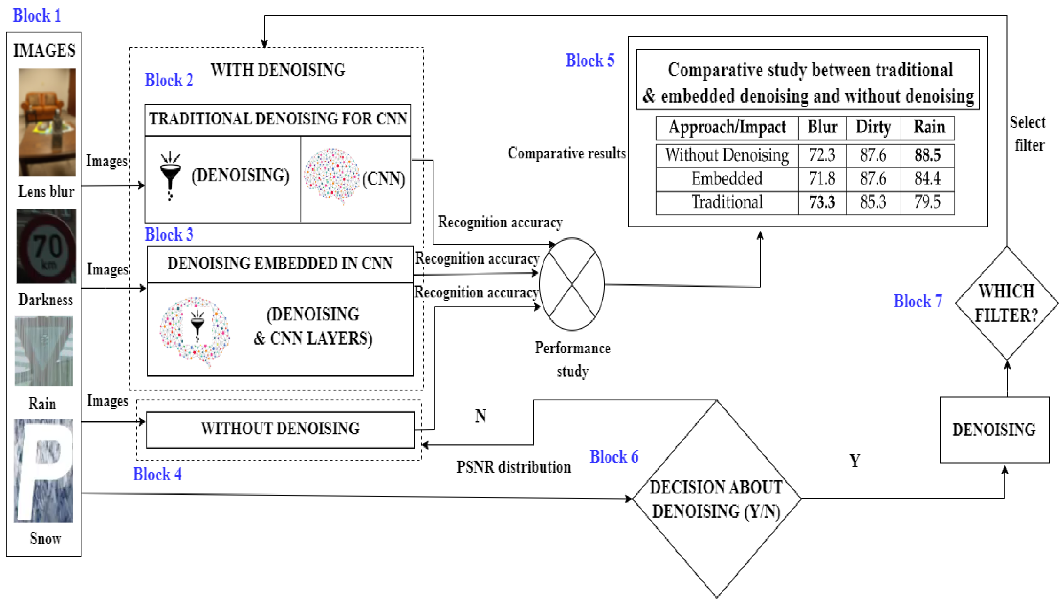
3.1. Overview of the Comparative Study

Figure 1 represents the schematic diagram of how we conduct the comparative performance study of CNN using traditional and embedded denoising against a baseline approach (without denoising) and present an approach to decide whether denoising is to be adopted.
  • For the traditional denoising approach, firstly, denoising is carried out separately with a filter as a pre-processing step. Secondly, denoised images are utilized in CNN for the performance study of a particular application (e.g., object recognition), which is mentioned in block 2 of Figure 1.
  • For the embedded denoising approach, denoising and recognition are carried out together with CNN. In this approach, a filter is embedded into the CNN model. An example of embedding a filter into CNN is illustrated in block 3 of Figure 1.
  • Block 4 is without denoising, where no filtering is carried out representing a baseline approach for this comparative study. The recognition accuracy is measured without any filtering with CNN.
  • Input images (refer to block 1 of Figure 1) are also used for deciding whether denoising will be adopted for a particular application based on the decision derived in the Y/N form (refer to block 6 of Figure 1). Once the decision is adopted for filtering and if the type of noise present is unknown, we can compare the PSNR before and after noise removal and choose the filter that provides the best performance in improving image quality after filtering, which is given in block 7 of Figure 1.
  • This comparative study will produce comparative results. A sample of the comparative results obtained from the performance study in the form of recognition accuracy with the traditional, embedded, and without denoising approaches is shown in Figure 1, which is detailed in Section 4.

3.2. Methodology for Comparative Analysis on Denoising in CNN-Based Approaches

We use median and Gaussian filter because the bilateral filter takes more processing time in comparison with the median filter. The kernel size of the median and Gaussian filter must be a positive odd integer.
For assessing the impact of filtering on recognition accuracy, any suitable approach that can represent the differences between the overall image quality of a dataset before and after denoising can be used. However, we aim to leverage the distribution of image quality based on a histogram as a histogram can visually depict the comparative overall image quality of the dataset well before and after filtering. Moreover, the histogram can be used to assess quality improvement.
For such an assessment, we can apply the following two principles:
  • Higher frequency values for higher PSNRs.
  • If the histogram is right skewed.
Based on these two principles, we can qualitatively and quantitatively assess whether the overall image quality is improved after filtering and thus decide whether denoising and the type of filtering will be employed.

3.3. Datasets

We use two datasets for denoising: CURE-TSR [18] and CURE-OR [19]. Both these dataset contains real and synthetic images embedded with noise. In both datasets, the percentage of noise level is not given. However, both datasets have five different levels of noise: (i) extreme less, (ii) less, (iii) moderate, (iv) high, and (v) extreme high. In CURE-TSR, different traffic sign types include speed limit, goods vehicles, no overtaking, no stopping, no parking, stop, bicycle, hump, no left, no right, priority to, no entry, yield, and parking. We use all of the traffic sign images, including the images shown in Figure 1 for various environmental impacts such as lens blur, lens dirtiness, rain, shadow, darkness, and snow. For camera impacts, we cover the two most prominent impacts such as lens blur and lens dirtiness. In CURE-OR, various classes include 23 categories of toys, 10 categories of personal items, 14 categories of office, 27 household categories, 10 categories of sports/entertainment, and 16 health categories. In this dataset, there is a total of 100 classes, while CURE-TSR contains 14 classes of different traffic signs. All of the images for lens blur, lens dirtiness, salt and pepper noise, contrast, overexposure, and underexposure impacts are used from the CURE-OR dataset, which includes all 100 object classes. From the literature, it is evident that the complex/cluttered backgrounds make object recognition difficult [53]. Therefore, to present the type of background of the CURE-OR dataset images, an example of a set of images having their background is shown in Figure 2.
We utilize 36,458 training and 16,670 test images for each environmental and camera impact to test the accuracy of the traffic sign detection CNN model. On the other hand, we use 11,220 training and 3750 test images for the CURE-OR dataset. The images without denoising and with denoising using median and Gaussian filter for impacts shadow, lens blur, and lens dirty are mentioned in Figure 3, Figure 4, and Figure 5, respectively.

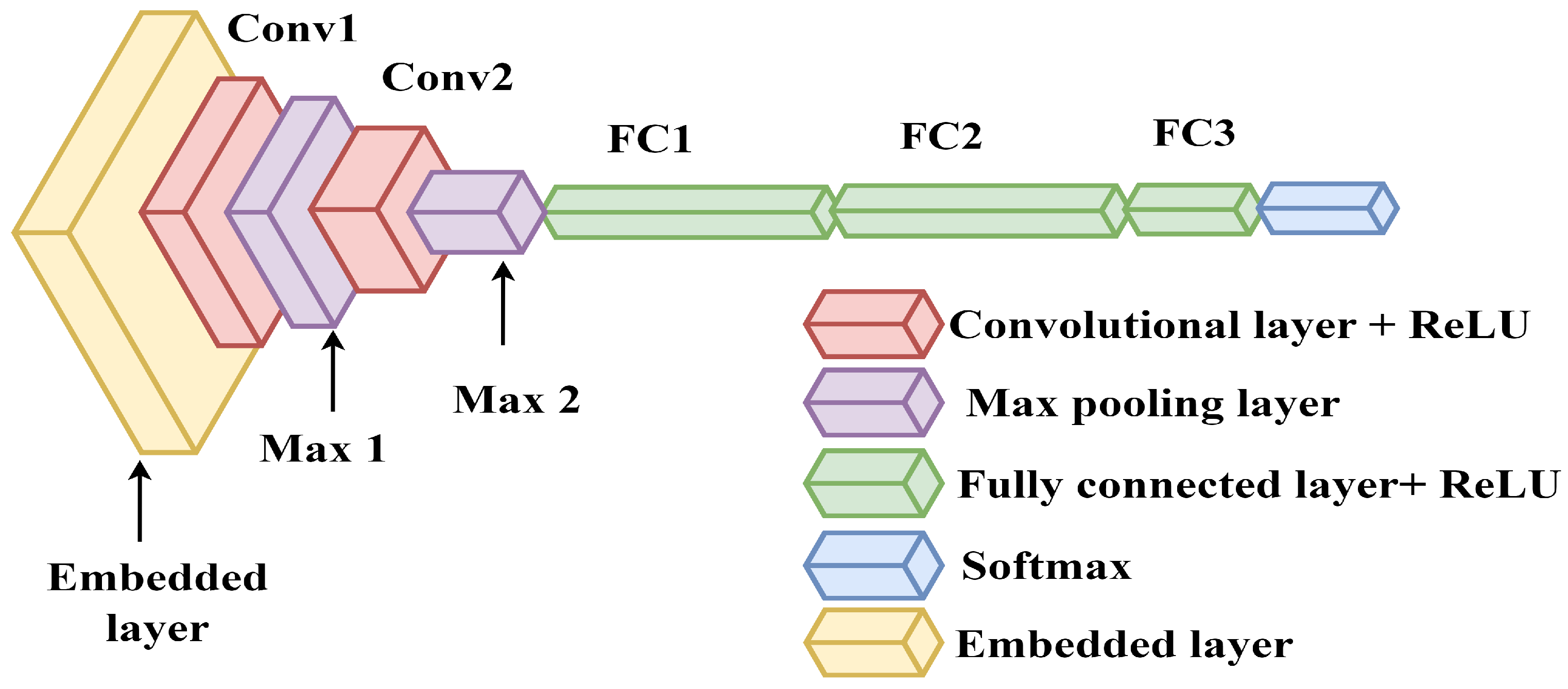
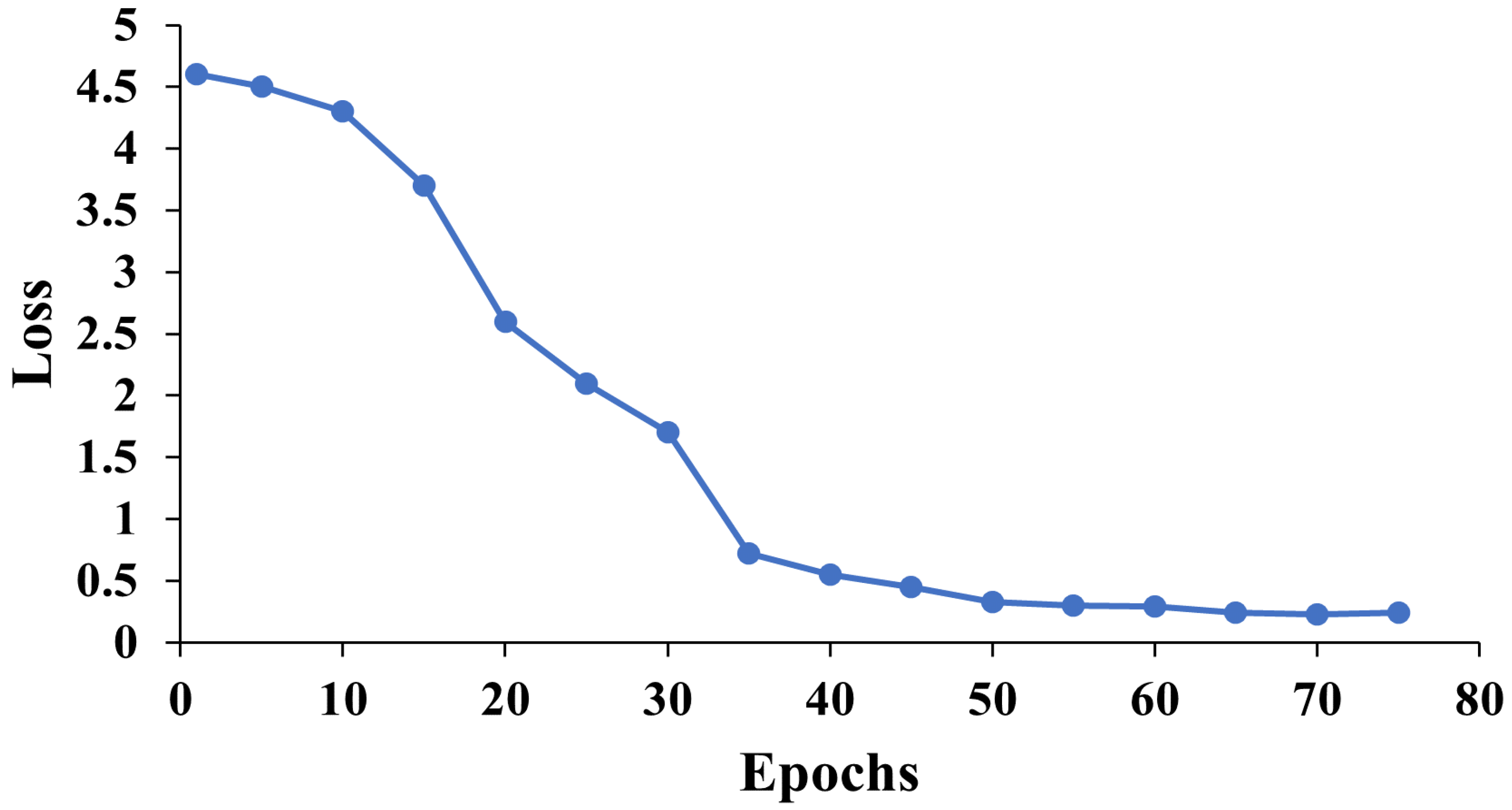
3.4. Description of CNN Model and Their Parameters

For evaluating the traffic sign and object recognition accuracy, we use a CNN model because it was introduced mainly for image processing applications and shows its potential efficacy in object recognition [18]. This model has less computational complexity, which is one of the major requirements for many real-time image recognition applications like live traffic sign detection used in autonomous vehicles. For traditional denoising, in general, a CNN comprises convolutional layers, pooling layers, fully connected layers, and a softmax layer for generating output.
As per [18], Figure 6 shows that the CNN model contains two convolutional and pooling layers followed by three fully connected layers. A filtering layer can be incorporated in any position of the CNN model but before the Softmax layer. However, in Figure 6 we embed an extra denoising layer of Gaussian or median filter, which is the first layer in the existing CNN model. This layer is embedded before the first convolutional layer of the CNN model. More embedded layers of Gaussian and median filters could be added to the CNN model. However, based on our experiments, we opted for only one embedded layer because the traffic sign and object recognition accuracy are almost the same as with embedding the first layer. Additionally, adding more filtering layers raises the computational complexity of the CNN model.

4. Results and Discussion

We calculate the Top-1 detection accuracy A (refer to Section 4.2) of CNN for various traffic signs and objects using the below-mentioned formula.
A = C / N
where C and N represent the number of correct predictions and the total number of predictions, respectively. We test the traffic sign detection accuracy and object detection accuracy of the traditional denoising approach and CNN-based embedded denoising approach against a baseline approach called without denoising.

4.1. Experimental Hardware and Software Settings

For our experimental purposes, we used the HP Zbook 15 G6 laptop, which has an in-built Intel CORE i7 vPro 9th Gen processor and an Nvidia Quadro T1000 processor. HP Zbook has 32 GB of physical memory. Our model was implemented using Python in Visual Studio Code software (version 1.41.1) with the support of the PyTorch library.
As per the methodology presented in Section 3.2, we implemented the traditional CNN model and the embedded CNN model using the architecture shown in Figure 6. The kernel size of the median filter used by us was 5, and kernel size = 15 for the Gaussian filter was used. We utilised a softmax classifier, which gives probabilities for each class label. As mentioned in Table 1, in our CNN model, we used 55 epochs for the CURE-TSR dataset as a reference from [18]. Also, for the CURE-OR dataset, we used 55 epochs because this number of epochs leads to a minimum loss, as is reflected in Figure 7. Figure 7 represents the epochs versus cross-entropy loss for the CURE-OR dataset using the validation set used in [18]. Cross-entropy loss continuously decreases from 4.6 to 0.3 until it reaches 55 epochs. After this, the loss remains almost the same even if the number of epochs increases. The learning rate was equal to 0.1. We used 256 batch sizes for our experiments.

4.2. Recognition and Computational Time Analysis for CURE-TSR

Recognition refers to the ability of a computer system to identify or classify objects, patterns, or features in an image or a video stream. Computational time analysis, on the other hand, refers to the process of measuring the time it takes for a computer system to perform a specific task, such as recognition or classification. This is an important metric in computer vision and pattern recognition as it can impact the overall performance and efficiency of the system. We calculate the traffic sign recognition accuracy and computational time for the CURE-TSR dataset. Note, in Table 2, Table 3, Table 4, Table 5 and Table 6, SD stands for standard deviation (SD), which represents the variation of Top-1 accuracy and computational time for each impact type.

4.2.1. Traffic Sign Recognition Accuracy

The recognition accuracy of CURE-TSR is mentioned in Table 3. The highest accuracy is given in bold in Table 3 and Table 5. The table shows the traffic sign recognition accuracy with both denoising approaches (embedded and traditional) using median and Gaussian filters and no denoising. To illustrate, in lens blur, the maximum recognition accuracy comes with the traditional denoising technique using a median filter, which is 73.3% compared with 70.3% accuracy obtained by the Gaussian filter, because Gaussian filters blur or smooth the image, which results in more blurring of images
Hence, the median filter is more effective at denoising lens blur in comparison with the Gaussian filter. Contrasted to lens blur, the Gaussian filter is effective in lens dirty, which is clearly reflected in Table 3. The traffic sign recognition accuracy is 88.1% for the embedded denoising approach with the Gaussian filter, which is maximum, as the Gaussian filter results in smoothening of the image while preserving the overall structure in lens dirtiness.
To perceive the overall detection accuracy and reliability of a particular approach, we calculate the mean value of Top-1 accuracies and their SD for all impacts. Overall, out of the without denoising, traditional, and embedded denoising approaches, traditional denoising with a median filter is superior to or similar to without denoising; it achieves maximum accuracy for the maximum number of impacts (2/6 impacts—lens blur and snow). Additionally, even though embedded denoising with median filter achieves the highest mean accuracy (76.5), traditional denoising with median filter obtains the second-highest mean accuracy (74.3) and the lowest SD (17.9) because the traditional denoising approach does not resize the images before denoising. However, the embedded approach requires the resizing of images before denoising, which leads to the loss of information and the addition of some redundant data into the existing database.
On the other hand, no denoising technique works in shadow and darkness. Table 2 shows the mean and SD of a particular image under different levels of impacts. It is depicted in Table 2 that the mean of gray-level values decreases as the level of impact such as darkness and shadow increases. For instance, in darkness, the value decreases continuously from 85.99 to 6.93 because a reduction in average gray value occurs as light intensity decreases, resulting in a reduction in overall image intensity. Similarly, in shadow, the mean value reduces from 117.7 to 69.49. It can be particularly challenging for filters like Gaussian and median to properly eliminate noise without altering the shadow regions since shadows change the overall brightness and contrast of an image as mentioned in Table 3. As a result, the shadow regions become blurry or smoothed [54]. In shadow, we achieve maximum recognition accuracy without any type of denoising, i.e., 89.6%. Likewise, the maximum accuracy without using any denoising approach is seen in darkness, which is 89.6% (refer to Table 3). Image noise and other artifacts may appear when an image is taken in low light or complete darkness because there may not be enough lighting to produce an accurate and well-exposed image. Gaussian and median filters may not be able to effectively remove the noise in these circumstances.
Another environmental impact is rain, where no denoising approach works. We attain the maximum accuracy (88.5%) of rain without using any denoising technique because rain streaks are often more complex and correlated and can extend across multiple pixels in a non-uniform manner. The median and Gaussian filters may not be effective at removing the specific type of noise caused by rain streaks. Specialized algorithms are required that are designed to specifically address this type of noise and separate it from the underlying image content [55].

4.2.2. Computational Time for Traffic Sign Recognition

The computational time of CNNs is influenced by various factors, such as the number of layers, the size of the input data, the number of filters in each layer, and the size of the filters. In these experiments, we refer to both training and testing time as computational time. In these experiments, we use the same number of layers, number of filters, and size of the filters. However, the difference is just the size of the input data, which is mentioned in Section 3.3. Note, in Table 3 and Table 4, SH stands for shadow and DK means darkness. In Table 4 and Table 6, we provide the bold text where the processing time is the lowest.
In lens blur, snow, and darkness, an embedded denoising approach with a median filter takes more computational time. However, in lens dirty, rain, and snow, the traditional denoising approach with a median filter takes maximum computational time, as is seen in Table 4. In all the environmental and camera impacts, the median filter takes more computational time than the Gaussian filter due to the way it processes data. We calculated the mean values and standard deviation of computational time in each denoising approach. Embedded denoising with a Gaussian filter takes less computational time (36.6 m) than embedded denoising with a median filter. Also, the standard deviation of the computational time of embedded denoising with a Gaussian filter is the smallest (1.03) among all other denoising approaches because a Gaussian filter replaces each pixel with a weighted average of its neighbors based on a Gaussian distribution, whereas a median filter replaces each pixel in an image with the median value of its neighboring pixels. The neighboring pixels must be sorted to obtain the median value, which is a computationally expensive procedure. The Gaussian weighted average, on the other hand, can be computed quickly because it just requires addition and multiplication operations.

4.3. Recognition and Computational Time Analysis for CURE-OR

In this section, we present the object recognition accuracy by CNN using various denoising approaches. We also present the computational time taken by CNN for object recognition. Note, in Table 5 and Table 6, S & P stands for salt and pepper noise, OE means overexposure, UE stands for underexposure, CT stands for contrast, and SD means standard deviation.

4.3.1. Object Recognition Accuracy

Table 5 shows the object recognition accuracy of CNN by using traditional and embedded denoising approaches with median, Gaussian, and without a filter. For instance, traditional denoising with a median filter has maximum object recognition accuracy for lens blur, which is 52.6%. Similar results were seen in the CURE-TSR dataset for lens blur. For impact contrast, the traditional denoising approach with a median filter has maximum accuracy, i.e., 60.4%. Contrast refers to the difference in brightness or color between various parts of an image. A Gaussian filter may actually make contrast problems worse by blurring the borders between contrasting regions.
In overexposure, the traditional denoising approach with a Gaussian filter has maximum object recognition accuracy, i.e., 47.6%. When an image’s brightness is too high, overexposure happens and features are lost in the highlights. When an image is overexposed, the brightest pixels may all have the same high value, which will act as the region’s median value. This means that applying a median filter will not change the value of these pixels and will not recover the lost details. Similarly, in underexposure, the maximum object recognition accuracy uses an embedded denoising approach with a Gaussian filter (50.7%). Median filters do not work in underexposure because when an image’s brightness is too low, underexposure happens and features are lost in the shadows. The pixels in the darkest regions of an underexposed image might all have the same low value, which will serve as the region’s median value. A median filter cannot restore the lost features because it will not alter the value of these pixels. Table 5 shows the traditional median and Gaussian produce maximum accuracy for the maximum number of impacts (4/6 impacts). When we compare the mean accuracy and SD, embedded Gaussian is the best, with mean accuracy and SD as 49.6 and 2.9, respectively, while the embedded median appears to be the worst (its respective mean accuracy and SD are 34 and 3.6). However, if we contrast traditional denoising against embedded denoising, traditional denoising, especially traditional Gaussian, shows superior results overall.

4.3.2. Computational Time for Object Recognition

Table 6 represents the computational time for object recognition by different denoising approaches. In terms of processing time, similar to the computational time of CURE-TSR, the traditional denoising approach with a median filter takes more time (66.7 m) than the embedded denoising approach (49.9 m) with a median filter. Also, embedded denoising (44.9 m) and traditional denoising (43.4 m) approaches with the Gaussian filter take less computational time because they require simple mathematical operations. We do not consider the pre-processing time for traditional denoising because in real/live systems we would have to apply denoising before we could run CNN.

4.4. Decision about Denoising Needs to Be Made

We compare the recognition accuracy with the quality of images through PSNR histograms. Various image quality assessment metrics exist such as PSNR, the structural similarity index measure (SSIM), and others to assess image quality. However, among them, PSNR is one of the most reliable and widely used image quality assessment metrics. As demonstrated in Figure 8, the recognition accuracy varies consistently with the PSNR values, and in general, accuracy increases with an increased PSNR value. To illustrate this, in lens blur with Gaussian filtering, the traffic sign recognition accuracy decreases from 87.6 to 85.3 as PSNR decreases from 31.83 to 28.05.
Therefore, to compare the quality of images, we used the PSNR of all images for a particular impact before and after Gaussian and median filtering through histograms. Note that each image has one PSNR value. As per the discussion of results from the CNN’s recognition accuracy, we realize that denoising with Gaussian and median filters decreases the recognition accuracy for some environmental and camera impacts compared to applying denoising in CNN. For example, in rain, shadow, and darkness, the recognition accuracy decreases with denoising approaches. The decrease in recognition accuracy shows that the application of Gaussian and median filters degrades the image quality rather than improving it. Therefore, we need some criteria to make a firm decision on whether we should use denoising or not.
We make a decision on assessing the image quality. If the image quality improves after using embedded and traditional denoising with Gaussian and median filters, then denoising works; otherwise, we should not adopt the particular method for denoising. As alluded to before, we choose PSNR as an image quality measure and the distribution (histogram) of PSNRs to show the comparative image quality with and without applying denoising.
Figure 9a shows the comparative histogram of PSNR values of underexposure before and after Gaussian denoising for the CURE-OR dataset. According to the two principles mentioned in Section 3.2, the histogram is right skewed and has higher frequency values for higher PSNR values such as 28.2 dB and 28.3 dB after Gaussian denoising. The right-skewed and higher frequency values of higher PSNRs vindicate that the overall image quality of the CURE-OR dataset in underexposure is improved after denoising with Gaussian filtering, i.e., the Gaussian filter is effective for the removal of underexposure. Parallely, Table 3 also shows that the highest (50.7%) and second highest (45.9%) object recognition accuracies produced by CNN are for embedded and traditional denoising with Gaussian filtering, respectively. Similarly, Figure 9b represents the histogram of PSNR values in underexposure before and after median denoising for the CURE-OR dataset. In comparison to Gaussian denoising, in this figure, the histogram is right-skewed (as it is shifted to a higher PSNR value, which is 28.3 dB) after denoising. However, higher frequency values do not exist for higher PSNRs (28.1 and 28.2 dB) after denoising. Only one principle is followed for the median filter, unlike the Gaussian filter, which follows both principles. To conclude, it is reflected from these histograms that the Gaussian filter is effective for the removal of underexposure. Table 5 also shows that the lowest (30.2%) and second lowest (32.1%) object recognition accuracies produced by CNN are for embedded and traditional denoising with median filtering, respectively.
Correspondingly, the comparative histogram of PSNR of lens blur is shown in Figure 10. As per the principle, the histogram after Gaussian filtering is not right-skewed and has less frequency at higher PSNRs (refer to Figure 10a). Table 5 also shows the lowest (39.2%) and second lowest (39.4%) object recognition accuracy in the CURE-OR dataset after embedded and traditional denoising with Gaussian filtering. It indicates that the overall image quality of the CURE-OR dataset in lens blur is not improved after denoising with Gaussian filtering, i.e., the Gaussian filter is not effective for the removal of lens blur. However, with median denoising, it is not either left or right-skewed, but it has more frequency at high PSNR (31 dB) values. In this instance, only one principle is followed. It can be concluded that either median denoising or no denoising works in lens blur. The results exactly correlate with Table 5, which shows that the highest object recognition accuracy (64.9%) by CNN is with using traditional denoising with a median filter, and the second highest is without denoising, which is 60.1%. This demonstrates that the overall image quality of the CURE-OR dataset in lens blur is improved after denoising with median filtering, i.e., a median filter is effective for the removal of lens blur.
In the CURE-TSR dataset, the histogram of the shadow is given in Figure 11. Figure 11a represents the PSNR distribution before and after Gaussian filtering. The histogram is not right skewed after Gaussian denoising and does not have a higher frequency at maximum PSNR values. Table 2 also exhibits the lowest (83.3%) traffic sign detection accuracy for the shadow in the CURE-TSR dataset. It concludes that the overall image quality of the CURE-OR dataset in shadow is improved after denoising with Gaussian filtering, i.e., the Gaussian filter is not effective for the removal of shadow. Similarly Figure 11b shows that it is not following the two above-mentioned principles mentioned in Section 3.2. The histogram after median filtering is not right-skewed and does not have high values at higher PSNRs (32 dB and 34 dB). As a consequence, the quality of images is not improved after denoising with a median filter. Similar results are shown in Table 5, where the no denoising approach has maximum traffic sign recognition accuracy, i.e., 92%.
This demonstrates that the overall image quality of the CURE-OR dataset in shadow is not improved after denoising with median or Gaussian filtering. Therefore, it is not recommended to use either embedded or traditional denoising with median or Gaussian filters.
Also, in the darkness, it is clear from Table 5 and Figure 12 that denoising is not working with either median or Gaussian filter. The value of maximum traffic sign recognition accuracy is 89.6 without a denoising approach. Also, the histogram does not follow the two principles of right skewing and high values at higher PSNRs. It elucidates that the overall image quality of the CURE-OR dataset in darkness is not improved after denoising with median or Gaussian filtering. Therefore, it is not recommended to use either embedded or traditional denoising with median or Gaussian filters for darkness.
As a consequence, through the comparison of recognition accuracy and PSNR distribution, we can conclude whether denoising needs to be adopted in particular environmental and camera impacts or not.

5. Conclusions

In this paper, we present traditional and embedded image-denoising approaches to analyze the performance of a deep learning algorithm called CNN. The performance of CNN is analyzed in terms of recognition accuracy and computational time. For this study, we use the CURE-TSR and CURE-OR datasets. We embed the Gaussian and median denoising filters because with the traditional approach, the results are almost the same in median and bilateral filters. Therefore, the Gaussian and median filters are used as these are more time-efficient among all three filters. The traditional denoising approach achieves high traffic recognition accuracy for more impacts than the embedded-based denoising approach. And the higher computational time is taken by both denoising approaches with a median filter compared to the Gaussian filter. The Gaussian filter is the most time-efficient filter to be used in denoising approaches. In this paper, for denoising embedded in CNN, we added an extra denoising layer. It is embedded as the first layer in the existing CNN model. However, we can add a denoising layer in any place before or after each convolution layer as well and will evaluate the results in the future. Moreover, the performance of denoising approaches has been evaluated using recognition accuracy. We present an approach to deciding whether decisioning will be adopted by leveraging the PSNRs distribution of images. The derived decisions verified the recognition accuracy for all the impacts of the two well-known image recognition datasets used in this paper. In the future, we aim to assess the impact of image denoising on various CNN-based image analysis applications such as smart agriculture and others where outdoor image capturing is required. This performance study has been conducted using traditional denoising approaches such as Gaussian and median filters. In this performance study, we embedded the filters into the CNN model, and these above-mentioned filters are used as a pre-processing step before finding the recognition accuracy using CNN in traditional denoising. CNN is mainly focused on calculating the traffic sign and object recognition accuracy. However, there are DL-based techniques especially using CNN dedicated to denoising that are available in the literature. For our future study, we will exploit these DL-based denoising techniques. In this study, we use CURE traffic signs and object recognition datasets. We will use other image recognition benchmark datasets applied in different applications in the future.

Author Contributions

Conceptualization, R.K. and M.I.; Methodology, R.K.; Software, R.K.; Validation, R.K.; Formal analysis, R.K.; Investigation, R.K.; Writing—original draft, R.K.; Writing—review & editing, R.K., G.K. and M.I.; Visualization, R.K.; Supervision, G.K. and M.I. All authors have read and agreed to the published version of the manuscript.

Funding

This research received no external funding.

Institutional Review Board Statement

Not applicable.

Informed Consent Statement

Not applicable.

Data Availability Statement

Data sharing not applicable.

Conflicts of Interest

The authors declare no conflict of interest.

References

  1. Juneja, A.; Kumar, V.; Singla, S.K. A systematic review on foggy datasets: Applications and challenges. Arch. Comput. Methods Eng. 2022, 29, 1727–1752. [Google Scholar] [CrossRef]
  2. Mehra, A.; Mandal, M.; Narang, P.; Chamola, V. Reviewnet: A fast and resource optimized network for enabling safe autonomous driving in hazy weather conditions. IEEE Trans. Intell. Transp. Syst. 2020, 22, 4256–4266. [Google Scholar] [CrossRef]
  3. Zhang, Y.; Carballo, A.; Yang, H.; Takeda, K. Perception and sensing for autonomous vehicles under adverse weather conditions: A survey. ISPRS J. Photogramm. Remote Sens. 2023, 196, 146–177. [Google Scholar] [CrossRef]
  4. Kaur, R.; Karmakar, G.; Xia, F. Evaluating Outdoor Environmental Impacts for Image Understanding and Preparation. In Image Processing and Intelligent Computing Systems; CRC Press: Boca Raton, FL, USA, 2023; pp. 267–295. [Google Scholar]
  5. Kaur, R.; Karmakar, G.; Xia, F.; Imran, M. Deep learning: Survey of environmental and camera impacts on internet of things images. Artif. Intell. Rev. 2023, 56, 9605–9638. [Google Scholar] [CrossRef]
  6. Bharati, S.; Khan, T.Z.; Podder, P.; Hung, N.Q. A comparative analysis of image denoising problem: Noise models, denoising filters and applications. In Cognitive Internet of Medical Things for Smart Healthcare; Springer: Berlin/Heidelberg, Germany, 2021; pp. 49–66. [Google Scholar]
  7. Elad, M.; Kawar, B.; Vaksman, G. Image Denoising: The Deep Learning Revolution and Beyond—A Survey Paper. arXiv 2023, arXiv:2301.03362. [Google Scholar] [CrossRef]
  8. Patil, R.; Bhosale, S. Medical image denoising techniques: A review. Int. J. Eng. Sci. Technol. (IJonEST) 2022, 4, 21–33. [Google Scholar] [CrossRef]
  9. Rama Lakshmi, G.; Divya, G.; Bhavya, D.; Sai Jahnavi, C.; Akila, B. A Review on Image Denoising Algorithms for Various Applications. In Proceedings of the Fourth International Conference on Communication, Computing and Electronics Systems: ICCCES 2022, Coimbatore, India, 15–16 September 2022; Springer: Berlin/Heidelberg, Germany, 2023; pp. 839–847. [Google Scholar]
  10. You, N.; Han, L.; Zhu, D.; Song, W. Research on image denoising in edge detection based on wavelet transform. Appl. Sci. 2023, 13, 1837. [Google Scholar] [CrossRef]
  11. Sehgal, R.; Kaushik, V.D. CT Image Denoising Using Bilateral Filter and Method Noise Thresholding in Shearlet Domain. In Emerging Technologies in Data Mining and Information Security: Proceedings of IEMIS 2022, Volume 1; Springer: Berlin/Heidelberg, Germany, 2022; pp. 99–106. [Google Scholar]
  12. Snehalatha, M.; Ramamurthy, N.; Swetha, K.; Vishnupriya, K.; Sreelekha, P.; Niharika, N. An Effective Image Denoising in Spatial Domain Using Bilateral Filter. J. Electron. Commun. Syst. 2022, 7, 9–14. [Google Scholar] [CrossRef]
  13. Liyanage, N.; Abeywardena, K.; Jayaweera, S.S.; Wijenayake, C.; Edussooriya, C.U.S.; Seneviratne, S. Making Sense of Occluded Scenes using Light Field Pre-processing and Deep-learning. In Proceedings of the 2020 IEEE REGION 10 CONFERENCE (TENCON), Osaka, Japan, 16–19 November 2020; pp. 538–543. [Google Scholar] [CrossRef]
  14. Duong, M.T.; Phan, T.D.; Truong, N.N.; Le, M.C.; Do, T.D.; Nguyen, V.B.; Le, M.H. An Image Enhancement Method for Autonomous Vehicles Driving in Poor Visibility Circumstances. In Proceedings of the Computational Intelligence Methods for Green Technology and Sustainable Development: Proceedings of the International Conference GTSD2022, Nha Trang City, Vietnam, 29–30 July 2022; Springer: Berlin/Heidelberg, Germany, 2022; pp. 13–25. [Google Scholar]
  15. Priyanka, S.A.; Wang, Y.K. Fully symmetric convolutional network for effective image denoising. Appl. Sci. 2019, 9, 778. [Google Scholar] [CrossRef]
  16. Tian, C.; Xu, Y.; Zuo, W. Image denoising using deep CNN with batch renormalization. Neural Netw. 2020, 121, 461–473. [Google Scholar] [CrossRef]
  17. Yang, L.; Fan, J.; Huo, B.; Li, E.; Liu, Y. Image Denoising of Seam Images With Deep Learning for Laser Vision Seam Tracking. IEEE Sens. J. 2022, 22, 6098–6107. [Google Scholar] [CrossRef]
  18. Temel, D.; Kwon, G.; Prabhushankar, M.; AlRegib, G. CURE-TSR: Challenging Unreal and Real Environments for Traffic Sign Recognition. arXiv 2019, arXiv:1712.02463. [Google Scholar] [CrossRef]
  19. Temel, D.; Lee, J.; AlRegib, G. CURE-OR: Challenging Unreal and Real Environment for Object Recognition. arXiv 2019, arXiv:1810.08293. [Google Scholar] [CrossRef]
  20. Fan, L.; Zhang, F.; Fan, H.; Zhang, C. Brief review of image denoising techniques. Vis. Comput. Ind. Biomed. Art 2019, 2, 7. [Google Scholar] [CrossRef]
  21. Gu, S.; Timofte, R. A brief review of image denoising algorithms and beyond. In Inpainting and Denoising Challenges; Springer: Berlin/Heidelberg, Germany, 2019; pp. 1–21. [Google Scholar]
  22. Monajati, M.; Kabir, E. A modified inexact arithmetic median filter for removing salt-and-pepper noise from gray-level images. IEEE Trans. Circuits Syst. II Express Briefs 2019, 67, 750–754. [Google Scholar] [CrossRef]
  23. Erkan, U.; Gökrem, L.; Enginoğlu, S. Different applied median filter in salt and pepper noise. Comput. Electr. Eng. 2018, 70, 789–798. [Google Scholar] [CrossRef]
  24. Kumar, S.; Bhardwaj, U.; Poongodi, T. Cartoonify an Image using Open CV in Python. In Proceedings of the 2022 3rd International Conference on Intelligent Engineering and Management (ICIEM), London, UK, 27–29 April 2022; IEEE: New York, NY, USA, 2022; pp. 952–955. [Google Scholar]
  25. Buades, A.; Coll, B.; Morel, J.M. A review of image denoising algorithms, with a new one. Multiscale Model. Simul. 2005, 4, 490–530. [Google Scholar] [CrossRef]
  26. Ahmad, K.; Khan, J.; Iqbal, M.S.U.D. A comparative study of different denoising techniques in digital image processing. In Proceedings of the 2019 8th International Conference on Modeling Simulation and Applied Optimization (ICMSAO), Manama, Bahrain, 15–17 April 2019; IEEE: New York, NY, USA, 2019; pp. 1–6. [Google Scholar]
  27. Han, Y.; Ye, J.C. Framing U-Net via deep convolutional framelets: Application to sparse-view CT. IEEE Trans. Med Imaging 2018, 37, 1418–1429. [Google Scholar] [CrossRef]
  28. Zhang, K.; Zuo, W.; Chen, Y.; Meng, D.; Zhang, L. Beyond a gaussian denoiser: Residual learning of deep cnn for image denoising. IEEE Trans. Image Process. 2017, 26, 3142–3155. [Google Scholar] [CrossRef]
  29. Liu, L.; Liu, B.; Huang, H.; Bovik, A.C. No-reference image quality assessment based on spatial and spectral entropies. Signal Process. Image Commun. 2014, 29, 856–863. [Google Scholar] [CrossRef]
  30. Vemulapalli, R.; Tuzel, O.; Liu, M.Y. Deep gaussian conditional random field network: A model-based deep network for discriminative denoising. In Proceedings of the IEEE Conference on Computer Vision and Pattern Recognition, Las Vegas, NV, USA, 27–30 June 2016; pp. 4801–4809. [Google Scholar]
  31. Plotz, T.; Roth, S. Benchmarking denoising algorithms with real photographs. In Proceedings of the IEEE Conference on Computer Vision and Pattern Recognition, Honolulu, HI, USA, 21–26 July 2017; pp. 1586–1595. [Google Scholar]
  32. Zhang, Q.; Xiao, J.; Tian, C.; Chun-Wei Lin, J.; Zhang, S. A robust deformed convolutional neural network (CNN) for image denoising. CAAI Trans. Intell. Technol. 2023, 8, 331–342. [Google Scholar] [CrossRef]
  33. Tai, Y.; Yang, J.; Liu, X.; Xu, C. Memnet: A persistent memory network for image restoration. In Proceedings of the IEEE International Conference on Computer Vision, Venice, Italy, 22–29 October 2017; pp. 4539–4547. [Google Scholar]
  34. He, K.; Zhang, X.; Ren, S.; Sun, J. Deep residual learning for image recognition. In Proceedings of the IEEE Conference on Computer Vision and Pattern Recognition, Las Vegas, NV, USA, 27–30 June 2016; pp. 770–778. [Google Scholar]
  35. Ronneberger, O.; Fischer, P.; Brox, T. U-net: Convolutional networks for biomedical image segmentation. In Proceedings of the Medical Image Computing and Computer-Assisted Intervention–MICCAI 2015: 18th International Conference, Munich, Germany, 5–9 October 2015; pp. 234–241. [Google Scholar]
  36. Huang, G.; Liu, Z.; Van Der Maaten, L.; Weinberger, K.Q. Densely connected convolutional networks. In Proceedings of the IEEE Conference on Computer Vision and Pattern Recognition, Honolulu, HI, USA, 21–26 July 2017; pp. 4700–4708. [Google Scholar]
  37. Gao, X.; Zhang, L.; Mou, X. Single image super-resolution using dual-branch convolutional neural network. IEEE Access 2018, 7, 15767–15778. [Google Scholar] [CrossRef]
  38. Liu, G.; Dang, M.; Liu, J.; Xiang, R.; Tian, Y.; Luo, N. True wide convolutional neural network for image denoising. Inf. Sci. 2022, 610, 171–184. [Google Scholar] [CrossRef]
  39. Zhang, K.; Zuo, W.; Zhang, L. FFDNet: Toward a fast and flexible solution for CNN-based image denoising. IEEE Trans. Image Process. 2018, 27, 4608–4622. [Google Scholar] [CrossRef]
  40. Saeed, A.; Nick, B. Real Image Denoising With Feature Attention. In Proceedings of the IEEE/CVF International Conference on Computer Vision (ICCV), Seoul, Republic of Korea, 27 October–2 November 2019; pp. 3155–3164. [Google Scholar]
  41. Guo, S.; Yan, Z.; Zhang, K.; Zuo, W.; Zhang, L. Toward convolutional blind denoising of real photographs. In Proceedings of the IEEE/CVF Conference on Computer Vision and Pattern Recognition, Long Beach, CA, USA, 15–20 June 2019; pp. 1712–1722. [Google Scholar]
  42. Alawode, B.O.; Alfarraj, M. Meta-Optimization of Deep CNN for Image Denoising Using LSTM. arXiv 2021, arXiv:2107.06845. [Google Scholar]
  43. Li, Z.; Wu, J. Learning deep CNN denoiser priors for depth image inpainting. Appl. Sci. 2019, 9, 1103. [Google Scholar] [CrossRef]
  44. Tian, C.; Xu, Y.; Li, Z.; Zuo, W.; Fei, L.; Liu, H. Attention-guided CNN for image denoising. Neural Netw. 2020, 124, 117–129. [Google Scholar] [CrossRef]
  45. Chaudhary, S.; Moon, S.; Lu, H. Fast, efficient, and accurate neuro-imaging denoising via supervised deep learning. Nat. Commun. 2022, 13, 5165. [Google Scholar] [CrossRef]
  46. Zhao, M.; Cao, G.; Huang, X.; Yang, L. Hybrid Transformer-CNN for Real Image Denoising. IEEE Signal Process. Lett. 2022, 29, 1252–1256. [Google Scholar] [CrossRef]
  47. Xue, T.; Ma, P. TC-net: Transformer combined with cnn for image denoising. Appl. Intell. 2023, 53, 6753–6762. [Google Scholar] [CrossRef]
  48. Zheng, Y.; Jiang, W. Evaluation of vision transformers for traffic sign classification. Wirel. Commun. Mob. Comput. 2022, 2022, 3041117. [Google Scholar] [CrossRef]
  49. Wang, H. Traffic Sign Recognition with Vision Transformers. In Proceedings of the 6th International Conference on Information System and Data Mining, Silicon Valley, CA, USA, 27–29 May 2022; pp. 55–61. [Google Scholar]
  50. Liang, L.; Deng, S.; Gueguen, L.; Wei, M.; Wu, X.; Qin, J. Convolutional neural network with median layers for denoising salt-and-pepper contaminations. Neurocomputing 2021, 442, 26–35. [Google Scholar] [CrossRef]
  51. Jin, L.; Zhang, W.; Ma, G.; Song, E. Learning deep CNNs for impulse noise removal in images. J. Vis. Commun. Image Represent. 2019, 62, 193–205. [Google Scholar] [CrossRef]
  52. Tian, C.; Zheng, M.; Zuo, W.; Zhang, B.; Zhang, Y.; Zhang, D. Multi-stage image denoising with the wavelet transform. Pattern Recognit. 2023, 134, 109050. [Google Scholar] [CrossRef]
  53. Golcarenarenji, G.; Martinez-Alpiste, I.; Wang, Q.; Alcaraz-Calero, J.M. Machine-learning-based top-view safety monitoring of ground workforce on complex industrial sites. Neural Comput. Appl. 2022, 34, 4207–4220. [Google Scholar] [CrossRef]
  54. Fattal, R.; Lischinski, D.; Werman, M. Gradient domain high dynamic range compression. In Proceedings of the 29th Annual Conference on Computer Graphics and Interactive Techniques, San Antonio, TX, USA, 23–26 July 2002; pp. 249–256. [Google Scholar]
  55. Shao, M.; Qiao, Y.; Meng, D.; Zuo, W. Uncertainty-guided hierarchical frequency domain transformer for image restoration. Knowl.-Based Syst. 2023, 263, 110306. [Google Scholar] [CrossRef]
Figure 1. Overview of the comparative study.
Applsci 13 11560 g001
Figure 2. Different backgrounds in CURE-OR dataset [19].
Applsci 13 11560 g002
Figure 3. Images of the shadow without denoising and denoising with median and Gaussian filter for CURE-TSR dataset. (a) Without filter. (b) After median filter. (c) After Gaussian filter.
Applsci 13 11560 g003
Figure 4. Images of lens blur without denoising and denoising with median and Gaussian filter for CURE-OR dataset. (a) Without filter. (b) After median filter. (c) After Gaussian filter.
Applsci 13 11560 g004
Figure 5. Images of lens dirty without denoising and denoising with median and Gaussian filter for CURE-OR dataset. (a) Without filter. (b) After median filter. (c) After Gaussian filter.
Applsci 13 11560 g005
Figure 6. Overview of the embedded denoising approach.
Applsci 13 11560 g006
Figure 7. Epochs vs. L=loss for CURE-OR dataset.
Applsci 13 11560 g007
Figure 8. Mean PSNR vs. recognition accuracy in CURE-TSR dataset. Here, LBWD: lens blur without denoising; LBM: lens blur with median filtering; LBG: lens blur with Gaussian filtering; LDWD: lens dirty without denoising; LDM: lens dirty with median filtering; LDG: lens dirty with Gaussian filtering; RWD: rain without denoising; RM: rain with median filtering; RG: rain with Gaussian filtering; SWD: shadow without denoising; SM: shadow with median filtering; SG: shadow with Gaussian filtering; DWD: darkness without denoising; DM: darkness with median filtering; and DG: darkness with Gaussian filtering.
Applsci 13 11560 g008
Figure 9. Comparative histogram of PSNR of underexposure without denoising and with Gaussian and median filtering for CURE-OR dataset. (a) Before and after Gaussian filtering. (b) Before and after median filtering.
Applsci 13 11560 g009
Figure 10. Comparative histogram of PSNR of lens blur without denoising and with Gaussian and median filtering for CURE-OR dataset. (a) Before and after Gaussian filtering. (b) Before and after median filtering.
Applsci 13 11560 g010
Figure 11. Comparative histogram of PSNR of the shadow without denoising and with Gaussian and median filtering for CURE-TSR dataset. (a) Before and after Gaussian filtering. (b) Before and after median filtering.
Applsci 13 11560 g011
Figure 12. Comparative histogram of PSNR of darkness without denoising and with Gaussian and median filtering for CURE-TSR dataset. (a) Before and after Gaussian filtering. (b) Before and after median filtering.
Applsci 13 11560 g012
Table 1. Various parameters and their type/values for CNN.
ParameterType/Value
Learning rate0.1
Epochs55
Batch size256
Activation functionReLU
ClassiferSoftmax
Convolutional layers3
Max-pooling2
Fully connected layers3
Table 2. Mean and standard deviation of gray level pixel intensities for a particular image having different levels of impacts for shadow and darkness. Here, Levels 1–5 represent the extent of impact starting from extreme low to extreme high. Here, the mean and standard deviation represent the impact of each level on the gray level pixel intensities of that image.
Impact LevelsDarknessShadow
Mean SD Mean SD
Without impact117.797.52117.797.52
Level 185.9971.36108.1289.07
Level 245.7537.8298.3781.51
Level 324.4920.2188.9176.86
Level 413.0410.7979.1374.5
Level 56.935.8469.4975.09
Table 3. Traffic sign recognition accuracy (%) of CNN in different environmental and camera impacts with various denoising approaches for CURE-TSR. Note, Acc. stands for accuracy, SH is shadow, and DK means darkness.
Acc. for Each Impact (%)Total
ImpactBlurDirtyRainSnowSHDKMeanSD
Approach
Without denoising72.387.688.51.99289.671.931.9
Embedded median71.887.684.435.690.789.276.519.33
Embedded Gaussian71.388.186.31.991.189.271.3131.7
Traditional median73.385.379.535.687.884.874.317.9
Traditional Gaussian70.380.474.91.983.31.952.135.7
Table 4. Computational time (minutes) for traffic sign recognition for different impacts with various denoising approaches in CURE-TSR. Here, mean and SD stand for the mean and standard deviation of the computational time for all impacts.
Computational Time for Each ImpactTotal
ImpactBlurDirtyRainSnowSHDKMeanSD
Approach
Without Denoising4645.6645.843.343.238.743.72.78
Embedded median50.54345.1944.344.446.645.62.64
Embedded Gaussian35.636.936.535.838.536.436.61.03
Traditional median46.251.354.443.344.743.247.14.62
Traditional Gaussian41.6515443.443.144.646.25
Table 5. Object recognition accuracy (%) of CNN for different impacts with various denoising approaches.
OR Accuracy for Each Impact (%)Total
ImpactBlurDirtyS & PCTOEUEMeanSD
Approach
Without Denoising52.635.8453.755.843.542.447.37.2
Embedded median32.834.441.431.334.430.2343.6
Embedded Gaussian49.146.250.45546.550.749.62.9
Traditional median52.635.650.560.434.432.144.210.7
Traditional Gaussian46.747.639.249.647.645.946.13.2
Table 6. Computational time (minutes) for object recognition for different impacts with various denoising approaches for CURE-OR. Here, mean and SD stand for the mean and standard deviation of the computational time for all impacts.
Computational Time for Each ImpactTotal
ImpactBlurDirtyS & PCTOEUEMeanSD
Approach
Without denoising60.141.843.546.34836.946.17.86
Embedded median40.442.443.86067.845.449.911.19
Embedded Gaussian39.461.341.848.537.541.244.98.83
Traditional median64.939.3118.464.847.665.566.727.55
Traditional Gaussian39.24340.337.635.465.243.410.95
Disclaimer/Publisher’s Note: The statements, opinions and data contained in all publications are solely those of the individual author(s) and contributor(s) and not of MDPI and/or the editor(s). MDPI and/or the editor(s) disclaim responsibility for any injury to people or property resulting from any ideas, methods, instructions or products referred to in the content.

