Model-Based Design of Aircraft Landing Gear System

Abstract

The aerospace industry is one of the leading figures in the development and improvement of techniques for the design of new products. One of the most promising developments of the last decades is the exploitation of digital models that make it possible to evaluate design solutions and simulate the behavior of the individual systems and their interactions. The goal is to be able to predict and analyze all aspects an aircraft much in advance of its industrialization in order to heavily reduce the time and costs of product development and to guarantee flexibility to test a multitude of solutions. The main issue in this context is the complexity of creating models that are capable of accurately sizing and simulating multiple interacting systems, thus considering the constraints imposed by the need for their mutual compatibility. The present contribution introduces two interconnected models regarding an aircraft system, in particular, the landing gear, that make it possible to size its main components and subsystems and to use the found parameters to populate a dynamic model that simulates the behavior of the aircraft during landing. These models provide a preliminary digitalization of the system itself and of the design process as well, thereby making it possible to define a potential configuration and to test it in a dynamic virtual environment, thus taking into account the interaction between the individual subsystems. The model was tested through three use cases, differentiated by class and scope, which made it possible to compare and validate the obtained results with actual values.

1. Introduction

Modern industrial products are smarter and more effective than in the past, but they sometimes exhibit a high level of complexity. Such complexity may derive from many different factors, such as from the many disciplines that are involved during its development, the constraints in terms of safety, the logistics of its supply chain, and many more. All of these are most certainly involved in the aerospace field, which is in charge of designing, manufacturing, and managing extremely complex products that must guarantee the highest possible level of safety and, at the same time, be able to carry out the given mission as efficiently and effectively as possible.

For this reason, it has become imperative to be able to reliably design aircraft systems and predict their behavior largely in advance with respect to their industrialization. Moreover, the interaction that arises between the multitude of systems is especially critical, and it must be solidly taken into account. In fact, properly designed systems and carefully set up models that reproduce a system allow designers to better understand what is the phenomenon they are dealing with, thus supporting them in their decisional path through the design activity and particularly in the trade-off of proposed layouts. Those aspects are crucial to move the main cost of development to the earliest phases of the product life cycle in order to avoid late changes in process that might exceedingly increase the financial investment [1].

One of the most important systems of an aircraft, thus making its definition in early development a priority, is the landing gear. The landing gear is the system in charge of supporting the aircraft when in contact with the ground. Therefore, it is active when the aircraft is parked, taxiing, taking-off, and landing. Among these phases, the harshest ones are takeoff and landing: the former is due to the large mass of the aircraft, and the latter is due to the high impact force that is generated when the aircraft comes into contact with the runway [2]. As such, when designing landing gear, these two are the phases which are considered for all the sizing calculations required.

In the last decades, there have been many methods, approaches and techniques that have been developed to carry out the design of such a complex system. Concerning its sizing, many works provide mathematical formulas for the estimation of the main parameters, thereby allowing the designer to gather a general picture of the system [3,4,5]. It is quite hard, however, to find a complete sizing workflow that makes it possible to estimate the necessary parameters to capture the behavior of the individual subsystems and their interaction. Regarding this purpose, many authors over the years have developed codes to predict the aircraft behavior during flight. For instance, Lynch [6] provides a program for the simulation of the aircraft dynamics during takeoff and landing. Lernbeiss and Plöchl [7] predicted the behavior of the shock absorber during landing. Kraft et al. [8] developed an experimental criterion for the analysis of the aircraft during ground maneuvers. Zegelaar performed an in-depth analysis of the dynamics of the pneumatic tire [9]; meanwhile, Tanner et al. studied the mechanical properties of the tires [10]. Finally, Daniels [11] validated numerical results with experimental data of the behavior of the landing gear main strut during landing. Those simulations, however, tended to work with already available, or at least sized, systems, to provide dynamic verification and/or characterization of the systems behavior or to focus on a specific subsystem of the landing gear. Other authors, meanwhile, such as Sonowal et al. [12] and Bailey [13], analyzed individual subsystems, thus providing sizing formulas, FEM/CFD simulations, or design guidelines, usually without considering the interaction with other subsystems.

From this perspective, the current contribution presents a sizing model in combination with a behavioral model that attempts to replicate the behavior and operation of the landing gear subsystems during the landing phase. More specifically, the first section describes the mathematical formulas used to dimension and characterize the wheels assembly, the braking system, and the shock absorber of the main landing gear. Thus, we provide a top-to-bottom workflow of the landing gear design. The computed parameters are then used for the setup of the behavior model, which is described in the next part. This model showcases the attitude of an aircraft during its landing, thereby taking into account the dynamics involved, so that the dynamics of the wheels, of the shock absorber, and of the actuation and control of the braking system can be accurately simulated. Such a model has been defined as a model-based systems engineering compatible model, thus allowing for the integration in a validation and verification (V and V) loop so that a finalized landing gear layout can be achieved more quickly and easily.

2. Preliminary Sizing Model

During the design and development of a new aircraft, multiple stages are encompassed, from marketing screening to experimental tests. One of the first phases, which makes it possible to gain a grasp of the general characteristics of the future aircraft, is the preliminary design phase. During this step, multiple evaluations and analyses are performed in order to obtain a first possible set of characteristics and to understand which kind and configuration is most suited to satisfy the customer’s needs.

As such, for this paper, a numerical code has been developed to perform a preliminary sizing of the components of the main landing gear. This code, developed in MATLAB^® 2023a [14], allows the designer to identify the main dimensions and parameters that characterize such important systems, which allow the interaction of the aircraft with the ground, thus allowing for aircraft parking, taxiing, takeoff, and landing. The code focuses on sizing the system components, i.e., the tires, the wheels, the brakes, and the shock strut, for the landing phase, as it can be considered the most critical of the aircraft mission and the most demanding for this specific system. The starting point of the sizing is the definition of aircraft parameters that allow for the computation of system-specific data. These parameters are reported in

Table 1. Initialization aircraft parameters for the landing gear components sizing.

System	Parameter	Description
Environment	$g=9.81$ m/s${}^2$	Gravity constant
	${\rho }_{air}=1.293$ kg/m${}^3$	Air density
	$T_{amb}=25$${}^{°}$C	Ambient temperature
	$H_{air}=10$ W/(m${}^2$·K)	Air convection coefficient
Aircraft	$M_{land}$ [kg]	Aircraft landing mass
	$V_{long}$ [m/s]	Longitudinal landing speed
	$V_{vert}$ [m/s]	Vertical landing speed
	$a_{land,m}$ [m/s${}^2$]	Mean landing deceleration
	$C_{lift}$	Lift coefficient
	$C_{drag}$	Drag coefficient
	$S_{wing}$ [m${}^2$]	Wing reference surface
	$d_{wheelbase}$ [m]	Landing gear wheelbase
	$d_{nose,CG}$ [m]	Nose-gear-to-CG distance
	$L{F}_a$	Aircraft load factor (lift-to-weight ratio)
Wheels and Tires	$N_{wheel}$	Number of main wheels
	$f_{roll}$	Rolling resistance coefficient
	$B_{dry}$, $C_{dry}$, $D_{dry}$, $E_{dry}$	Pacejka coefficients
	${\eta }_{tire}$	Tire efficiency
Brakes	${\rho }_{b,r}$ [kg/m${}^3$]	Brake rotors density
	${\rho }_{b,s}$ [kg/m${}^3$]	Brake stators density
	$C_b$ [J/(kg·K)]	Brake discs specific heat
	$k_b$ [W/(m·K)]	Brake discs thermal conductivity
	$N_{b,r}$	Number of brake rotors
	$f_{brake}$	Brake discs friction coefficient
Shock strut	$L{S}_{gear}$	Landing gear load factor
	${\rho }_{oil}$ [kg/m${}^3$]	Shock oil density
	$C_{dis}$	Orifice discharge coefficient
	${\eta }_{shock}$	Shock absorber efficiency
	$P_{static}$ [Pa]	Shock static pressure

, and they are classified based on the correlated component.

Once the initialization data have been completed, the preliminary sizing of the individual components can be performed. Unless otherwise indicated, all dimensions are in SI units.

2.1. Wheels and Tires Sizing

First of all, the wheels and tires of the aircraft must be dimensioned in order to provide the correct behavior of the aircraft during the ground maneuvers. More specifically, the tires and wheels of the main landing gear absorb most of the impact during landing and support the majority of the weight of the aircraft on the ground [12]. Therefore, it is fundamental to estimate the actual weight that the landing gear must carry. Based on the mass of the aircraft, it is possible to obtain the static load on each of the main wheels through the moments equilibrium, as the following equation from Currey [5] illustrates:

$$F_{main,vert}=\frac{M_{land}·g}{N_{wheel}}\frac{d_{nose,CG}}{d_{wheelbase}}$$

(1)

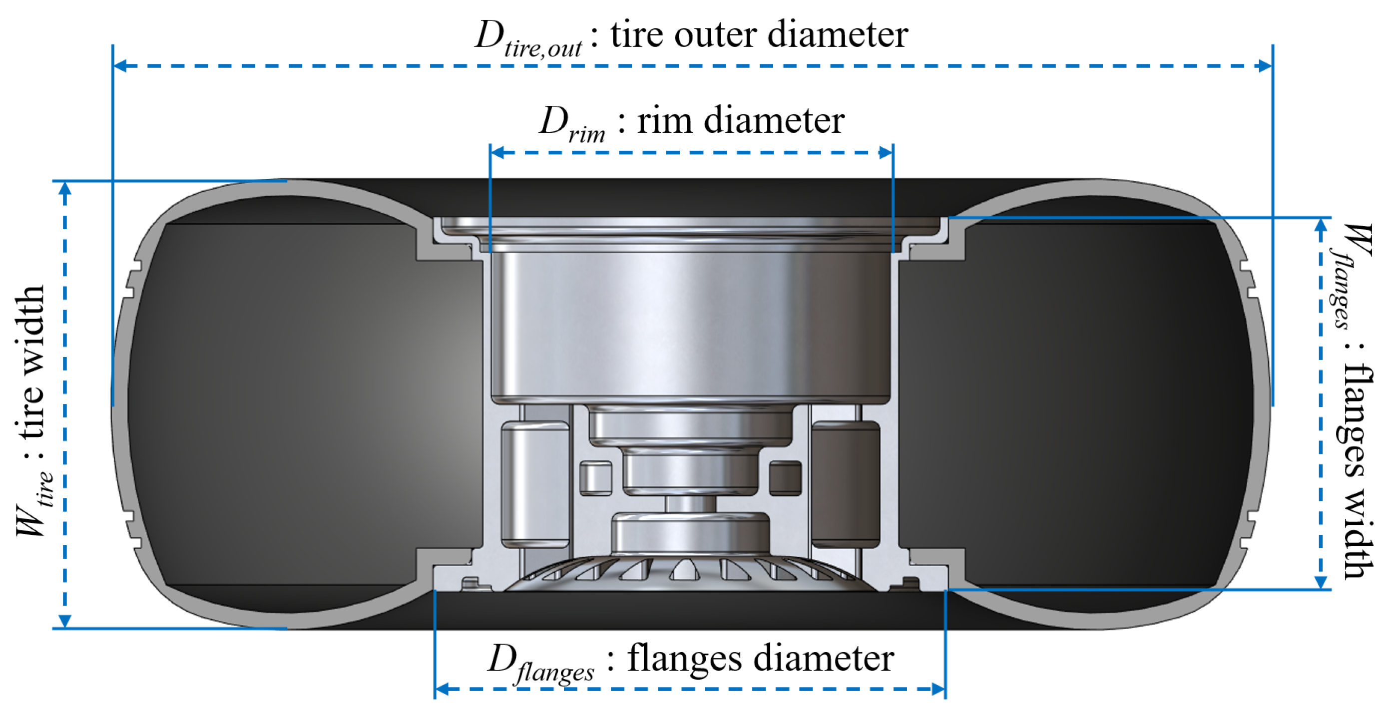
Based on this value, the main dimensions of the tires and wheels can be evaluated: in fact, each tire is characterized by an index called the rated load, which indicates the max vertical load applicable on the tire [15]. Therefore, a higher tire rated load will be able to cope with a higher aircraft mass. However, as can be seen in Figure 1, there are multiple dimensions that characterize wheels and tires, where each combination corresponds to a different rated load. Additionally, tire manufacturers employ the tire ply index $N_{ply}$ to characterize their products, which represents the strength of the tire.

Since there is no actual empirical formulation which makes it possible to find all the necessary values, it is more suitable to resort to the largely available catalogs from the tire manufacturers. Based on this approach, Sforza [4] has provided a formula to estimate the diameter of the wheel rim:

$$D_{rim}=1.4{\left(F_{main,vert}\frac{2.20468}{g}\right)}^{1/4}\left[\mathrm{in}\right]$$

(2)

The other fundamental values can be found utilizing the Goodyear tire catalog [16] as a database to create second-order polynomial regression models with respect to the fundamental parameter, i.e., the tire rated load, for each dimension:

$$Tireouterdiameter=D_{tire,out}=-0.0264F_{load}^2+2.0033F_{load}+15.8532\left[\mathrm{in}\right]R\text{-}square=89.15\%$$

(3)

$$Tirewidth=W_{tire}=-0.0056F_{load}^2+0.6993F_{load}+5.0774\left[\mathrm{in}\right]R\text{-}square=89.53\%$$

(4)

$$Tireplyindex=N_{ply}=-0.0236F_{load}^2+1.5917F_{load}+7.3648R\text{-}square=90.95\%$$

(5)

where $F_{load}=F_{main,vert}·{10}^{-5}$.

With the tire outer diameter, it is also possible to obtain the distance between the wheel rim flanges through another regression model:

$$W_{flanges}=0.0025D_{tire,out}^2+0.1010D_{tire,out}+1.9183\left[\mathrm{in}\right]R\text{-}square=99.08\%$$

(6)

Upon obtaining these dimensions, it is immediately possible to estimate the mass of the tires and the wheels. Again, Sforza [4] has provided two useful formulas:

$$m_{tire}=\frac{D_{tire,out}{N}_{ply}{W}_{tire}}{107}\left[\mathrm{lbs}\right]m_{wheel}=0.1\pi \left(D_{rim}{W}_{tire}+\frac{D_{rim}^2}{4}\right)\left[\mathrm{lbs}\right]$$

(7)

These masses then make it possible to compute the inertia of the wheel assembly through the following [17]:

$$I_{wheel}=I_{tire}+I_{rim}=m_{tire}{\left(\frac{D_{tire,out}}{2}\right)}^2+\frac{3m_{wheel}}{4}{\left(\frac{D_{rim}}{2}\right)}^2$$

(8)

It is very important noticing that, once the dimensions of the wheel assembly have been found, it is possible to compute the tire rated load $R{L}_{tire}$, which makes it possible to verify the load capacity of the new tire compared to the aircraft mass. Regarding this purpose, Schmidt [3] has provided an equation to find such a value:

$$R{L}_{tire}=A_{cp}\left(P_{tire}+P_{tire,c}\right)\left[\mathrm{lbs}\right]$$

(9)

where $A_{cp}$ is the contact patch area, $P_{tire}$ is the tire pressure index, and $P_{tire,c}$ is the equivalent pressure of the tire carcass.

First, the contact patch can be found as follows:

$$A_{cp}=0.77\pi d\sqrt{\left(D_{tire,m}-d\right)\left(W_{tire}-d\right)}\left[{\mathrm{in}}^2\right]$$

(10)

where $d=b\left(D_{tire,m}-D_{rim}\right)/2$ indicates the static deflection of the tire, $D_{tire,m}=D_{tire,out}-D_{rim}$ is the mean tire diameter, and b is the fractional tire deflection, which is usually assumed to equal $0.32$ [3].

Then, the pressure index can be computed:

$$P_{tire}=\frac{40R_e{T}_o{N}_e}{S{F}_o}$$

(11)

where $R_e=1.475-0.331L_r$ is a parameter that is dependent on the tire lift ratio, $L_r=D_{tire,m}/D_{rim}$, which is related to the tire construction, $T_o$, which is equal to $4.4$ and is a tire type-related parameter; $N_e=N_{plies}-0.4$, $S=\left(\frac{D_{tire,m}-D_{rim}}{4}\right)\left(2.5+\frac{D_{rim}}{2D_{tire,m}}\right)$ and $F_o=-1.623104\times {10}^{-7}{D}_{rim}^5+1.463062\times {10}^{-5}{D}_{rim}^4-5.607522\times {10}^{-4}{D}_{rim}^3+0.01288401D_{rim}^2-0.197904D_{rim}+2.567982$ express the tire operating factor.

Finally, the tire carcass equivalent pressure can be found as follows:

$$P_{tire,c}=\frac{10.4N_{plies}^2}{W_{tire}^2}$$

(12)

If the computed rated load of the tire $R{L}_{tire}$ is higher than the load applied on each tire, the tire/wheel combination found may be considered satisfactory.

Finally, it is possible to estimate the elastic stiffness of the sized tire from the following equation:

$$k_{tire}=\frac{M_{land}g}{N_{wheel}{S}_{tire,rest}}$$

(13)

where $S_{tire,rest}=\frac{1}{3}\left(\frac{D_{tire}}{2}-\frac{D_{rim}}{2}\right)$ is the assumed tire deflection at rest [4].

2.2. Brakes Sizing

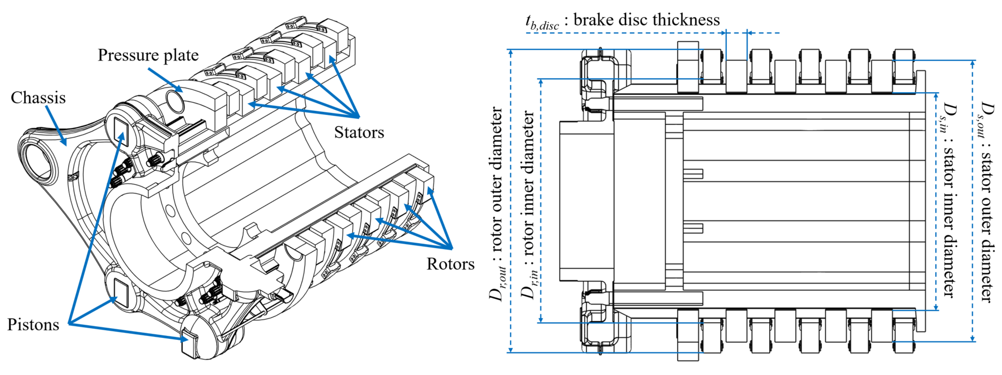
While the tires and wheels of the landing gear provide support to the aircraft when in contact with the ground, it is fundamental for the aircraft to be able to come to a complete stop in due time. This is true not only when the aircraft is landing, but also during taxi maneuvers and in case of a rejected takeoff. The main system in charge of this operation is the landing gear braking system, an example of which is reported in Figure 2.

The most common type of braking system employs disc rotors, which are integral to the rotating wheels, which, when the braking action is required, are compressed between stator discs, fixed to the landing gear, by applying hydraulic pressure through a pressure plate. The friction generated by the discs converts the kinetic energy of the aircraft into thermal energy, thus slowing it down. The energy to be converted during landing can be easily computed as follows:

$$E_{land}=\frac{1}{2}{M}_{land}{V}_{long}^2$$

(14)

Since mechanical brakes convert kinetic energy into thermal energy, the main issue that must be taken into account is the brake temperature. Based on the material, the thermal characteristics of the brake pack can largely vary. For instance, steel brakes (very common and cheaper solution) cannot withstand temperatures higher than 1000 °C; meanwhile, carbon discs are a more expensive solution but can manage temperatures of 1800 °C [18]. Therefore, the energy requirement during landing with respect to the minimum thermal mass of the brakes can be found depending on the material employed:

$$m_{brake,req}=\frac{E_{land}}{C_b\left(T_{b,des}-T_{amb}\right)}$$

(15)

where $C_b$ is the specific heat capacity of the brake material, and $T_{b,des}$ is the design brake temperature (i.e., the desired brake temperature at the end of the braking phase).

Although the required brake mass provides an indication as to the characteristics of the brakes to be designed, it does not allow for the actual sizing of the system. To this end, Bailey [13] has provided formulas that make it possible to estimate the characteristic diameters of the brake discs, based on the dimensions of the housing wheel, which are previously sized:

$$Rotorouterdiameter=D_{r,out}=0.788D_{rim}+2.322\left[\mathrm{in}\right]$$

(16)

$$Rotorinnerdiameter=D_{r,in}=0.6645D_{rim}-2.361\left[\mathrm{in}\right]$$

(17)

$$Statorouterdiameter=D_{s,out}=0.7091D_{rim}+2.286\left[\mathrm{in}\right]$$

(18)

$$Statorinnerdiameter=D_{s,in}=0.417D_{rim}+0.391\left[\mathrm{in}\right]$$

(19)

Based on these equations, the lateral areas of the brake rotors and stators are calculated follows:

$$A_{b,r}=\pi \frac{D_{r,out}^2-D_{r,in}^2}{4}{A}_{b,s}=\pi \frac{D_{s,out}^2-D_{s,in}^2}{4}$$

(20)

Then, the thickness of the discs can be computed. Since the disc must fit inside the wheel rim, a good approximation would be to consider the thickness of the disc pack $t_{b,pack}=0.75W_{flange}$. The thickness of each disc is then found though the expression $t_{b,disc}=t_{b,pack}/(N_{b,r}+N_{b,s})$, where $N_{b,s}$ is the number of stator discs, which is assumed to be $N_{b,r}+1$. These dimensions allow us to find the actual mass of the brakes:

$$m_{brake,act}=\left({\rho }_{b,r}{A}_{b,r}{N}_{b,r}+{\rho }_{b,s}{A}_{b,s}{N}_{b,s}\right)t_{b,disc}{N}_{wheel}$$

(21)

which should be higher than the requested mass computed in Equation (15).

In order to evaluate the performance of the designed brake pack, the lining loading may be computed as follows:

$$L{L}_{brake}=\frac{E_{land}}{A_b{N}_{b,i}{N}_{wheel}}$$

(22)

where $A_b$ is the contact surface between a rotor and stator discs pair, and $N_{b,i}=2N_{b,r}$ is the number of braking interfaces. It represents the amount of mechanical energy converted into thermal energy per unit of braking surface, thus indicating the stress applied on the brakes [19].

The last sizing parameter for the braking system is the actuation force required to stop the aircraft. Such a value can be estimated based of the desired mean deceleration during braking, which makes it possible to find the required braking torque:

$${\tau }_{brake,req}=\frac{M_{land}{a}_{land,m}{D}_{rim}}{2N_{wheel}}$$

(23)

Using Equation (23), based on the assumption of constant wear on the discs [20], the required actuation force can be computed:

$$F_{brake,act}=\frac{4{\tau }_{brake,req}}{N_{b,i}{f}_{brake}(D_{brake,out}+D_{brake,in})}$$

(24)

where $D_{brake,out}=min(D_{r,out},D_{s,out})$ and $D_{brake,in}=max(D_{r,in},D_{s,in})/2$ are, respectively, the outer and inner diameters of the braking surface.

2.3. Shock Strut Sizing

The last component of the main landing gear is the shock strut. This element connects the wheel assembly to the rest of the airframe and includes the retraction mechanism and the shock absorber. The shock absorber has the main function of absorbing the impacts that the aircraft is subjected to when in contact with the ground [12]. The most critical impact is the touchdown during the landing phase. Therefore, it is fundamental to size such a component to cope with the heavy loads arising from this event.

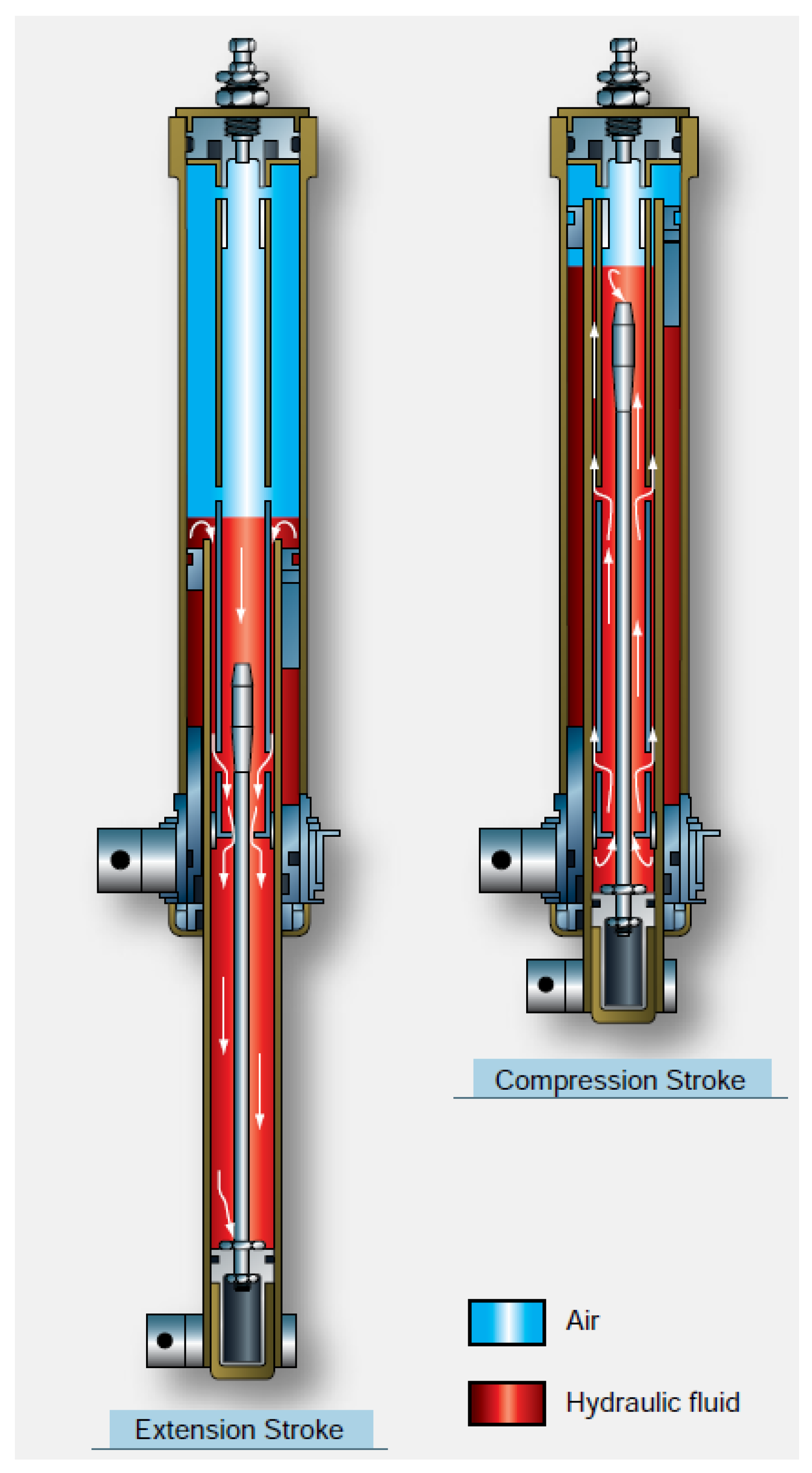
One of the most common technological solutions adopted for this role is the oleopneumatic absorber, which can be visualized in Figure 3. It can be simplified as a cylinder with a sliding piston, which separates the cylinder onto two chambers, connected by an orifice on the piston itself. Inside, two fluids are present: a compressible gas that acts as a pneumatic spring and oil, which, when the absorber is actuated, tends to flow through the orifice, thereby acting as the damping agent.

The first factor to estimate is the maximum stroke of the shock absorber. Multiple sources [4,5] provide a similar formulation to estimate it:

$$S_{shock}=\frac{V_{vert}^2}{2g}+S_{tire,rest}\frac{1-L{F}_a-L{F}_{lg}{\eta }_{tire}}{L{F}_{lg}{\eta }_{shock}-1+L{F}_a}$$

(25)

where $L{F}_{lg}$ is the landing gear loading factor, which is expressed as the ratio between the maximum applied load on the landing gear and the aircraft weight.

Then, the piston area can be found as follows:

$$A_{piston}=\frac{M_{land}g}{N_{shock}{P}_{shock,s}}$$

(26)

where $N_{shock}$ is the number of shock struts (usually two), and $P_{shock,s}$ is the shock pressure at rest, which can be assumed to be equal to 1500 psi. Additionally, the orifice area $A_{or}$ may be assumed to be $2\%$ of the piston area.

Using the calculated piston area, it is then possible to estimate the volume of the main chamber of the shock absorber in the static, fully compressed and fully extended positions:

$$V_{shock,s}=A_{piston}{S}_{shock,e}+V_{shock,c}$$

(27)

$$V_{shock,c}=0.1A_{piston}{S}_{shock}$$

(28)

$$V_{shock,e}=A_{piston}{S}_{shock}+V_{shock,c}$$

(29)

where $S_{shock,e}$ is the shock travel from the fully extended to the rest position, which could be assumed as $S_{shock}/3$.

Finally, since the shock absorber acts as an elastic and damping element, the damping coefficient and elastic stiffness can be estimated. The damping coefficient can be computed from the heaviest impact on the shock, i.e., the touchdown, as follows:

$$c_{shock}=\frac{{\rho }_{oil}}{2}{A}_{piston}{V}_{vert}{\left(\frac{A_{piston}}{C_{dis}{A}_{or}}\right)}^2$$

(30)

while the elastic stiffness can be estimated from Boyle’s law [22]:

$$k_{shock}=A_{piston}\frac{P_{shock,e}{V}_{shock,e}}{V_{shock,s}{S}_{shock,e}}$$

(31)

where $P_{shock,e}$ is the shock pressure when fully extended, which can be assumed to be $P_{shock,s}/4$ [5].

3. Dynamic Verification Model

Once all of the previously presented computations have been carried out, a preliminary configuration of the landing gear in terms of the size and characteristics is available. The next step would be to test if the newly designed components are actually capable of carrying out their function. One of the most useful methods to reach such a goal is the use of time-dependent dynamic models. These kind of models make it possible to simulate the behavior of complex systems, including their reciprocal interactions, during a defined mission. Such a dyanmic is true also for aircraft systems, which are highly integrated and interdependent, and, as seen in Equation (2), each is in charge of a specific function.

When considering the entire flight envelope that usually characterizes a typical mission of an aircraft, the landing phase is a very minor one in terms of the time and distance covered. This is especially true when larger-sized aircraft, designed for longer missions, are considered. However, it is actually described as the most problematic phase on the entire mission due to the difficulty of the maneuver and the overall criticality in terms of safety [23]. For this reason, a highly granular dynamic model for the prediction of the landing behavior of an aircraft has been developed. The software chosen for this task is the Simulink^® (Version 10.7; MathWorks, 2023) software for its attitude to model even highly complex systens and complete integration with the MATLAB^® environment. Such interconnection allows for seamless transfer of the parameters computed by the preliminary sizing script into the dynamic model. As such, the latter may be employed to test the landing performance of any kind of aircraft, regardless of its size or intended use. This model is comprised of multiple sections, witheach dedicated to a different aspect of the landing phase of the aircraft and the landing gear subsystems. More specifically, in the order with which each will be discussed, it includes:

• The longitudinal dynamics block;
• The vertical dynamics block;
• The landing gear block:

  -

  The main wheels:

  ∗

  The brake pack;

  ∗

  The tire/road interface;

  -

  The braking system control.

3.1. Aircraft Dynamics

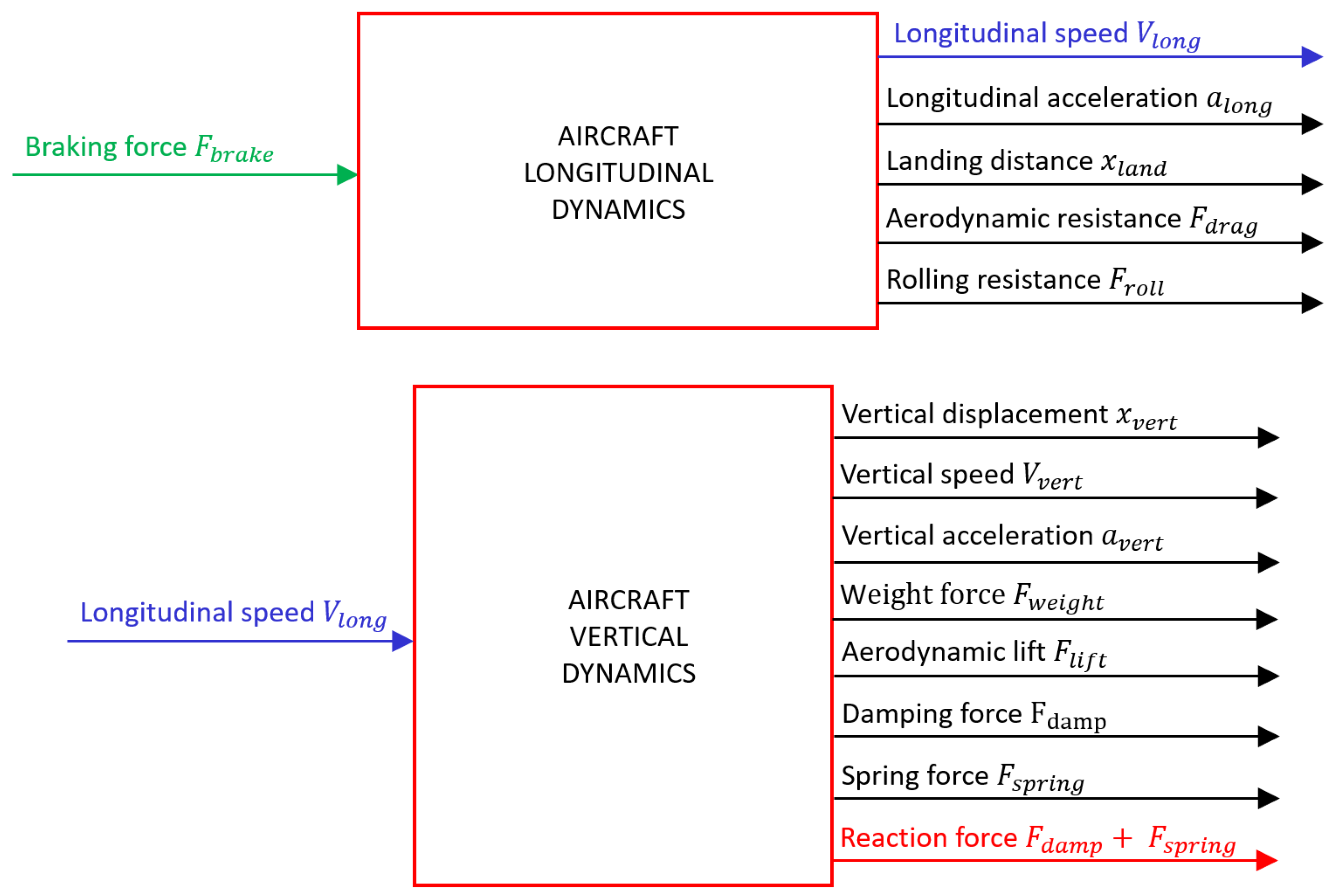
The aircraft is considered to be a point-mass system. Due to the lack of aircraft rolling motion in the model, each wheel can be considered in the same exact conditions, and, therefore, the simulation of just one wheel, when properly scaled in terms of forces, is sufficient to capture the entire system. Even without the inclusion of the rolling motion, the need for an analysis of the dynamics of the aircraft is clear, at least in terms of longitudinal and vertical behavior. Due to the phase we are considering, the dynamics can be compared to car dynamics, since we are dealing with only the longitudinal and vertical motion [24]. To this end, two subsystems in Simulink^® have been included, which are dedicated to the simulation of such characteristics of the aircraft. These elements are described in Figure 4.

As can be noticed, a few variables are computed in these blocks. For what concerns the longitudinal dynamics, three are the forces considered: the aerodynamic resistance, which is defined as

$$F_{drag}=\frac{1}{2}{\rho }_{air}{S}_{wing}{C}_{drag}{V}_{long}^2;$$

(32)

the rolling resistance, which is defined as

$$F_{roll}=M_{land}·g·f_{roll};$$

(33)

and the braking force $F_{brake}$, which will be described later. These forces provide the longitudinal equilibrium of the aircraft during landing, which is defined as follows:

$$\frac{\partial {\dot{x}}_{land}}{\partial t}=\frac{-F_{brake}-F_{drag}-F_{roll}}{M_{land}}$$

(34)

which computes the longitudinal acceleration $a_{long}$ and, thanks to a first and second integration, makes it possible to obtain the longitudinal velocity $V_{long}$ and the landing distance $x_{land}$ of the aircraft. For the sake of simplicity, the thrust of the propellers have not been taken into account, considering that the engines when landing should be at idle—if not providing a reverse thrust—or, in case of engine failure, the aircraft should be capable of stopping even without reverse thrust.

In a similar manner, the vertical dynamics block computes the forces involved in the equilibrium of the aircraft, from which its motion can be described. The forces involved in this case are the aerodynamic lift, which is defined as

$$F_{lift}=\frac{1}{2}{\rho }_{air}{S}_{wing}{C}_{lift}{V}_{long}^2;$$

(35)

the weight of the aircraft, which is equal to

$$F_{weight}=M_{land}·g;$$

(36)

and the reaction forces due to the presence of the landing gear, which act as a spring–damper system that is characterized by a damping coefficient $c_{shock}$ and a spring stiffness $k_{shock}$, which have been computed by the sizing script. These forces define the following equilibrium:

$$\frac{\partial {\dot{x}}_{vert}}{\partial t}=\frac{F_{weight}-F_{lift}-c_{shock}·V_{vert}-k_{shock}·x_{vert}}{M_{land}}$$

(37)

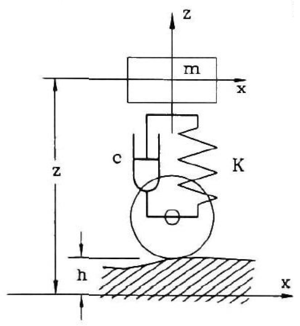
where the vertical acceleration $a_{vert}$, the vertical velocity $V_{vert}$, and the vertical displacement $x_{vert}$ can be found and where $c_{shock}·V_{vert}=F_{damp}$ is the damping force and $k_{shock}·x_{vert}=F_{spring}$ is the spring force. It can be noticed that the system considered in the vertical direction has a single degree of freedom, which is equivalent to the one defined in Figure 5. As such, the tires of the landing gear have been considered as rigid bodies for simplicity.

3.2. Landing Gear Model

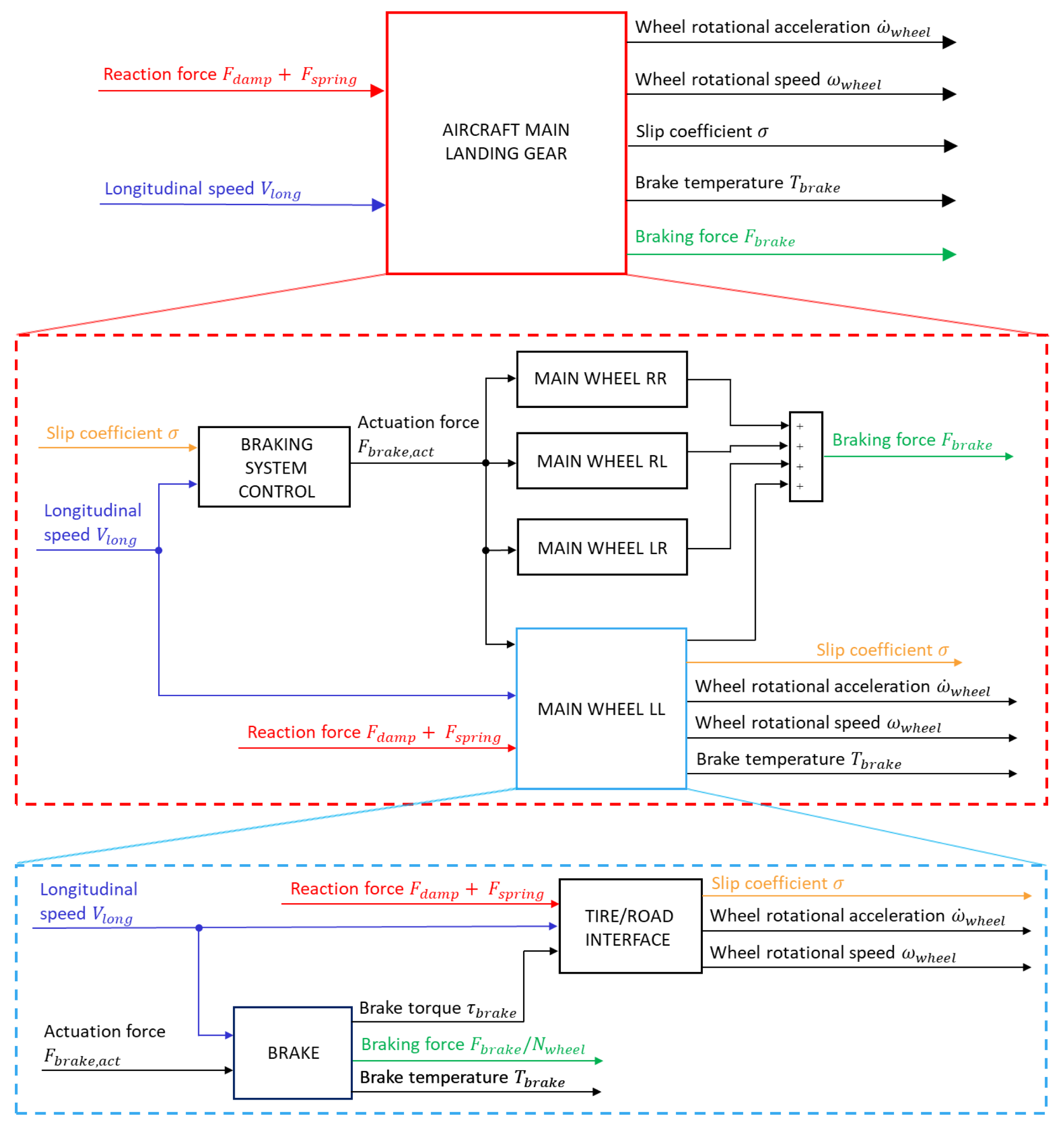
With the longitudinal and vertical dynamics implemented, the next step was to model the main subsystems of the landing gear. The shock absorber has already been described in the previous section, since it is the main element to consider for the vertical dynamics of the aircraft during landing. Therefore, the wheel assembly and the braking system have been modeled in a dedicated block. The resulting subsystem for the landing gear is reported in Figure 6.

In particular, the presence of the “Braking system control” block can be noticed, which is a subsystem dedicated to the definition of a control logic for the actuation of the braking system, which will be showcased later. The other ones are the “Main Wheel” blocks, with each representing one wheel of the main landing gear. As stated before, due to the simplifications employed in this model, the wheels can be considered to be equal to each other, and, therefore, it is sufficient to capture the behavior of a single wheel. Such a division has been included to enable the further deepening of the model fidelity in the future. As such, the “Main Wheel LL” subsystem will be considered for the current application. This element is further composed of two subsystems: the “Brake” subsystem, which is dedicated to the analysis of the brake pack of the wheel, and the “Tire/Road interface” subsystem, which is dedicated to the modeling of the interaction between the tire and the road surface.

3.2.1. Wheel Assembly

As introduced earlier, the wheel assembly of the main landing gear is modeled in the “Main Wheel LL” subsystem. This element, which can be seen in Figure 6, receives the following as input:

• the actuation force $F_a$ of the brake calipers, which is previously sized;
• the longitudinal speed of the aircraft $V_{long}$;
• the total reaction force of the landing gear $F_{vert}$, which is computed as the sum of the damping force and spring force from the “Vertical Dynamics” subsystem.

These inputs are used to compute the following outputs:

• the braking force on a single wheel, which is intended as $F_{brake}/N_{wheel}$;
• the longitudinal slip coefficient of the tire, which is defined as ${\delta }_{long}$;
• the wheel rotational speed ${\omega }_{wheel}$ and the acceleration $\dot{{\omega }_{wheel}}$;
• the brake discs temperature, which is defined as $T_{brake}$.

The first subsystem of the “Main Wheel LL”, again reported in Figure 6, is dedicated to the interface model between the tire and road. This block implements the rotational equilibrium of the wheel in order to obtain its behavior during landing. Such a model makes it possible, therefore, to add control logic to the braking system, which makes it possible to avoid certain unwanted phenomena, such as the lock of the wheel due to the excessive braking torque applied by the brakes. Such an equilibrium is found using the following equation:

$$\frac{\partial {\omega }_{wheel}}{\partial t}=\frac{-\frac{F_{vert}}{N_{wheel}}{\mu }_{long}{R}_{main}-{\tau }_{brake}}{I_{wheel}}$$

(38)

where $N_{wheel}$ is the number of wheels of the main landing gear, $R_{main}$ is the effective tire radius, ${\tau }_{brake}$ is the braking torque on the single wheel, $I_{wheel}$ is the moment of inertia of the wheel, and ${\mu }_{long}$ is the longitudinal friction coefficient. This last term represents the ratio between the longitudinal force exerted on the wheel and the vertical force applied on it. Therefore, the first term in the numerator of Equation (38) is the torque exerted on the wheel by its interaction with the road. The longitudinal force coefficients can be found through many methods. In the current application, the model used is the Pacejka “magic formula” [25], which makes it possible to find the longitudinal friction coefficient of the wheel based on the slip coefficient. It is defined as follows:

$${\mu }_{long}\left(\sigma \right)=D_{dry}sin\left(C_{dry}{tan}^{-1}(B_{dry}\sigma -E_{dry}(B_{dry}\sigma -{tan}^{-1}\left(B_{dry}\sigma \right)))\right)$$

(39)

where $B_{dry}$, $C_{dry}$, $D_{dry}$, and $E_{dry}$ are coefficients experimentally obtained relative to the road conditions, and $\sigma$ is the longitudinal slip coefficient, which is defined as follows:

$$\sigma =\frac{R_{main}{\omega }_{wheel}-V_{long}}{V_{long}}\mathrm{for}\mathrm{braking}\mathrm{conditions}$$

(40)

The road coefficients have been set for “dry tarmac” conditions. Due to the unavailability of experimental coefficients specific to the tires found with the preliminary sizing script, the same coefficients have been used for every simulation.

All of these equations have been implemented in the subsystem (with Equations (39) and (40) in the “Slip + Pacejka” subsystem), thereby iterating the computed longitudinal friction coefficient at every integration step for the computation of the wheel dynamics.

The other subsystem composing the landing gear is the “Brake”, which is in charge of modeling the behavior of the brake pack of a main gear wheel. More specifically, it simulates two main characteristics of the brakes: the braking torque generated (and, consequently the braking force) and the temperature reached by the brake discs during braking. The braking torque has been obtained based on the assumption of “constant wear” on the braking surface of the discs [20], which makes it possible to find it from the following:

$${\tau }_{brake}=F_{brake,act}{f}_b\frac{r_o+r_i}{2}{N}_b$$

(41)

where $f_b$ is the friction coefficient of the discs, $r_o=\frac{min(D_{r,out},D_{s,out})}{2}$ and $r_i=\frac{max(D_{r,in},D_{s,in})}{2}$ are, respectively, the outer and inner radii of the braking surface, and $N_b$ is the number of braking surfaces (equal to double the number of rotor discs).

The braking torque ${\tau }_{brake}$ is then divided by the effective rolling radius of the tire, thus making it possible to find the braking force $F_{brake}$ acting on one wheel. This equation is also implemented in the other “Main wheel” subsystems and, when all summed together, provides the total braking force of the aircraft, which is then used for the longitudinal equilibrium.

The braking force is also multiplied by the longitudinal speed of the aircraft, thus obtaining the instantaneous braking power $P_{brake}$, which is converted into thermal power by the brakes themselves. Therefore, if the thermal equilibrium of the brake discs is considered, their temperature evolution can be found as in Equation (42). For the current application, each brake disc is considered to be a uniform thermal mass affected by the natural air convection:

$$\frac{\partial T_{brake}}{\partial t}=\frac{\frac{P_{brake}}{N_b}-(T_{brake}-T_{air})2H_{air}\pi r_o{t}_b}{{\rho }_b{t}_b{A}_b{C}_b}$$

(42)

where $T_{air}$ is the environmental temperature, $H_{air}$ is the natural air convection coefficient, $t_b$ is the thickness of a brake disc (rotor and stator discs thickness are assumed to be the same), ${\rho }_b$ is the disc density, $A_b$ is the braking surface, and $C_b$ is the specific heat capacity of the disc.

By then integrating Equation (42), the instantaneous temperature of the brake is found.

3.2.2. Braking System Control

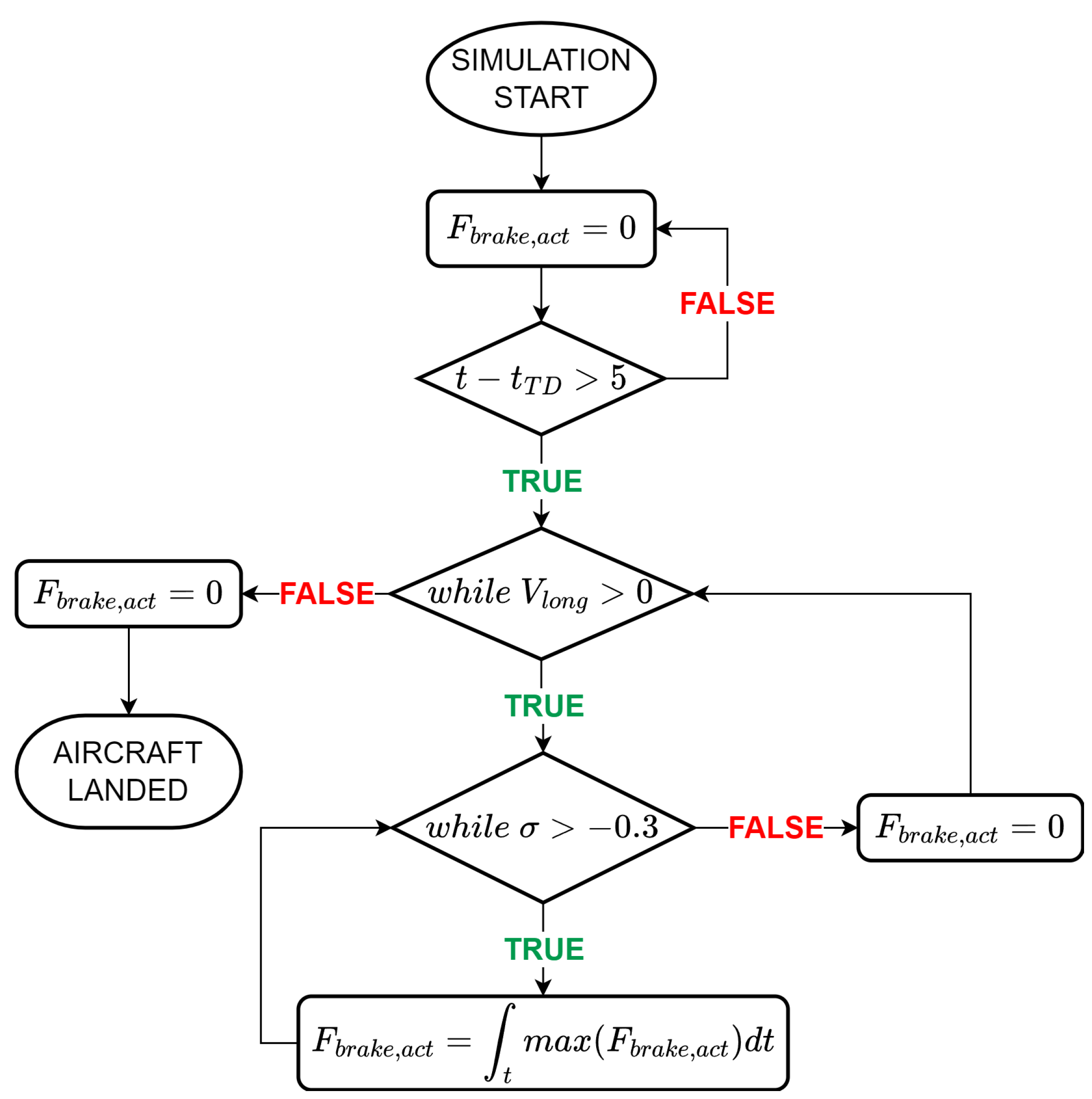
To obtain a simulation of the braking system that is closer to the real application, a control logic for the said system has been implemented in the “Braking system control” block. As can be seen in Figure 7, three checks are defined. First, a time delay in the braking action with respect to the wheels touching the ground, equal to 5 s, is included. This is done in order to allow the aircraft to achieve vertical stability before actual braking, and because during the very first moments of landing, the aerodynamic drag tends to provide a higher braking contribution.

The next one causes the interruption of the braking action when the aircraft speed is equal to zero (necessary just to avoid divisions by zero). Finally, a switch monitors the slip coefficient of the wheels and, when it goes below $-0.3$, the braking action is stopped. This last one simulates the control logic of an antiskid system, which, in real applications, avoids the locking of the wheels, which is a phenomenon that heavily reduces the braking capability of the aircraft and its stability on the runway. By removing the braking action when the slip coefficient goes below a certain value, where the wheel is very likely to lock, such a risk is very much reduced.

Apart from this kind of control, this subsystem also provides the signal for the actuation force applied on the disc brakes. Since the actuation of the brake is never instantaneous, when the braking action is requested, it is supplied as a linearly increasing signal up to the maximum value defined during the sizing of the system. As can be seen in the diagram, whenever the antiskid control is activated, the actuation force is reset again to zero, thus restarting the linear increase of the actuation force.

4. Simulation Results

Once the model has been set up, it is possible to run the simulation to capture the behavior of the aircraft during landing. Regarding this purpose, once the main aircraft data has been defined, the sizing script is run, which will then automatically populate the dynamic model with the necessary computed parameters, thus allowing for the execution of the dynamic simulation of the landing phase. Since the model uses multiple integrators, it is required to define the integration settings. It was decided to employ an “ode1 (Euler)” fixed-step solver. Regarding the integration step, a value of $T_{step}=0.0001$ s was set. Such a value makes it possible to maintain a good quality of the simulation and a low simulation time (a couple of seconds).

From the simulation, it was then possible to extract some relevant curves that show the behavior of the aircraft. To demonstrate the flexibility of the models, three test cases have been employed with very different sizes and missions: an ATR 42-600 (manufactured by ATR, Blagnac, France), which is a regional twin turboprop transport; a Boeing 737-600 (manufactured by The Boeing Company, Chicago, IL, USA), which is a twin turbofan airliner; and a McDonnell-Douglas F-15D (manufactured by McDonnell Douglas Corporation, Saint Louis, MO, USA), which is a military fighter. The relative numerical results from the preliminary sizing and from the dynamic simulations are reported in

Table 2. Numerical results obtained for the three aircraft test cases.

	ATR 42-600		F-15D		B737-800
	Actual	Computed (Error *)	Actual	Computed (Error *)	Actual	Computed (Error *)
MTOW [kg]	16,900		30,844		79,002
MLW [kg]	16,400		20,185		66,349
$d_{wheelbase}$ [m]	8.78		7.50		15.60
$d_{nose,CG}$ [m]	8		7		15
$x_{land}$ from TD [m]	661 **	730 (+10.4%)	784 **	1008 (+28.6%)	1280 **	1399 (+9.3%)
$x_{land}$ from Alt = 15 m [m]	966	1035 ** (+7.1%)	1100	1324 ** (+20.4%)	1634	1753 ** (+7.3%)
$V_{long}$ [m/s]	62.0		64.3		72.0
$V_{vert}$ [m/s]	3.05		3.05		3.05
$N_{wheel}$	4		2		4
$D_{rim}$ [in]	16.00	13.34 (−16.6%)	18.00	16.81 (−6.6%)	21.00	19.17 (−8.7%)
$N_{ply}$	12	13 (+8.3%)	26	21 (−19.2%)	28	27 (−3.6%)
$D_{tire,out}$ [in]	31.80	22.84 (−28.2%)	34.50	32.11 (−6.9%)	44.50	40.74 (−8.4%)
$W_{tire}$ [in]	8.53	7.57 (−11.3%)	8.40	11.06 (+31.7%)	14.80	14.65 (−1.0%)
$R{L}_{tire}$ [lbs]	11,000	10,992 (−0.1%)	30,100	27,030 (−10.2%)	44,700	45,000 (+0.7%)
$W_{flanges}$ [in]	7.00	5.53 (−21.0%)	7.50	7.74 (+3.2%)	10.50	10.18 (−3.0%)
$m_{tire}$ [kg]	19.00	9.52 (−49.9%)	36.80	31.62 (−14.1%)	91.00	68.29 (−25%)
$m_{wheel}$ [kg]	19.50	20.71 (+6.2%)		36.55	36.30	53.11 (+46.3%)
$k_{tire}$ [N/m]		999,760		1,528,150		1,782,600
$N_{b,r}$	2		4		4
${\rho }_{b,r}$ [kg/m${}^3$]	≈8000		≈1800		≈1800
${\rho }_{b,s}$ [kg/m${}^3$]	≈8000		≈1800		≈1800
$D_{r,out}$ [m]	<0.3777	0.3259	<0.4255	0.3954	<0.4928	0.4427
$D_{r,in}$ [m]		0.1651		0.2237		0.2636
$D_{s,out}$ [m]		0.2983		0.3608		0.4034
$D_{s,in}$ [m]		0.1512		0.1879		0.213
$t_{b,pack}$ [m]	<0.1778	0.0702	<0.1905	0.1474	<0.2667	0.1939
$t_{b,disc}$ [m]		0.0140		0.0164		0.0215
$m_{brake,act}$ [kg]		31.44		41.65		33.29
$L{L}_{brake}$ [J/m${}^2$]		3.03 $\times {10}^7$		4.15 $\times {10}^7$		7.34 $\times {10}^7$
$F_{brake,act}$ [N]		9291		11,426		18,771
$T_{brake}$ [${}^{°}$C]		370		931		1505
$S_{shock}$ [m]		0.4149		0.4051		0.3945
$A_{piston}$ [m${}^2$]		0.0078		0.0191		0.0315
$c_{shock}$ [Ns/m]		88962		218,990		359,910
$k_{shock}$ [N/m]		738,180		1,861,200		3,141,000

Model inputs are reported in black, sizing results in blue, dynamic model outputs in red. * With respect to actual values; ** Estimated values.

.

This table provides a synthesis of the results obtained through the models, including a comparison of the computed data with the actual characteristics of the real aircraft. A few considerations could be made regarding the accuracy the model:

• The landing performance: In terms of prediction of the landing distance from touchdown, the model tended to overestimate it. This is potentially related to how the aerodynamic performance has been implemented: in fact, during landing, an aircraft deploys flaps and ailerons, which highly increase aerodynamic drag; meanwhile, due to the unavailability of detailed aerodynamic maps, the drag was considered to be constant throughout the simulation.
• The tire/wheel sizing: Regarding the tire and wheel sizing values, the results are quite comparable to the actual ones. The larger difference is noticeable for the ATR 42-600, which could be solved with an improvement of the regression models for lower values of tire rated load. In any case, this latter value was found within $10\%$ of the real value, thus making it possible to assume that the found tire/wheel combination is still suitable for the specific application. In terms of masses, instead, it seems that the model needs an important tuning, considering that the formulas used only allow for a high level estimation, which does not take into account the material properties of the components.
• The brake sizing and performance: For what concerns the brake sizing, it is quite difficult to retrieve actual data. However, we can verify that the sized component is compatible with the available space provided by the actual wheels of the aircraft. Meanwhile, the temperatures achieved during landing are in line with what can be expected from the capabilities of the chosen materials, as presented in Section 2.2.
• The shock sizing and performance: Finally, the comparison of the sized shock absorber with actual values suffered from a similar unavailability of data as the brakes, thereby making it difficult to confirm them with certainty. However, it can be noticed that, as expected, there was a clear correlation between the shock parameters and the mass of the aircraft: in fact, the piston area, the spring stiffness, and the damping coefficient tended to increase with higher mass; meanwhile, the shock travel reduced. The increase of the first three quantities was clearly related to the need to absorb the heavier landing impact characterizing an aircraft of a larger mass. The reduction of shock travel is instead related to the higher deformation that affect the tires of a heavier aircraft, thereby prompting the need to have a lower shock travel to avoid contact of the underbody with the ground.

With regard to the dynamic model, it is then possible to plot numerous aircraft characteristics, thereby allowing the designer to further understand the aircraft performance and behavior.

4.1. Longitudinal Dynamics

The first set of curves obtained from the dynamic model are the longitudinal forces and kinematic behavior of the aircraft, which are, respectively, reported in Figure 8 and Figure 9.

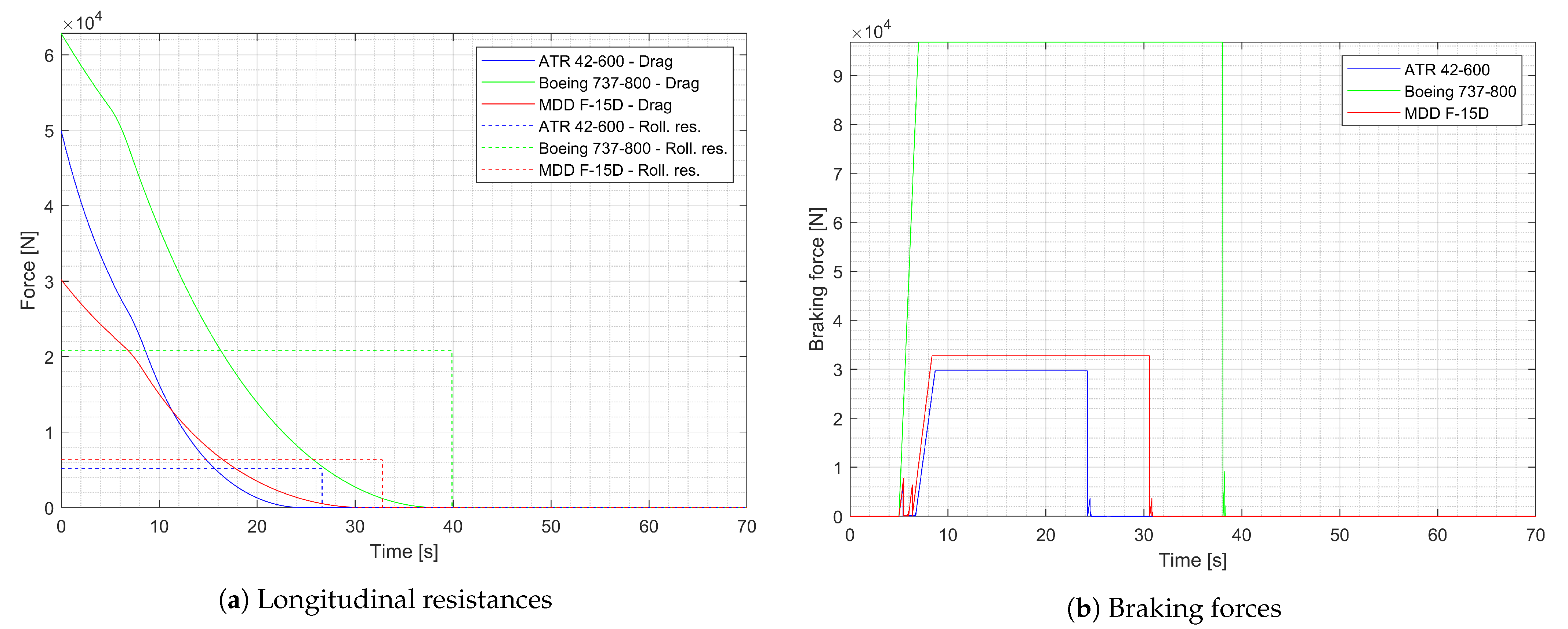
From Figure 8a, we can confirm the behavior of the aerodynamic and rolling resistance trend of the three aircraft: the former shows an exponentially decreasing behavior, due to its proportionality to the square value of the aircraft speed, while the latter presents a constant value, thereby showing the simplification of a constant rolling coefficient. The curve shown in Figure 8b is the braking force: we can see that the actuation started at 5 s from touching the ground due to the imposed actuation delay. It then took a few more seconds to reach a constant actuation. In all three cases, the linearly increasing braking force was appreciable, which was derived from the ramp signal used to provide the actuation force on the brakes, which then saturated at the maximum imposed value. A similar trend can also be found in literature [7,26]. Additionally, regarding the ATR42-600 and the MDD F-15D curves, the intervention of the antiskid logic was evident in the first few seconds of the braking phase: an alternating curve was noticeable due to the disengagement of the brakes returning the braking force to zero, which was due to the insufficient vertical force on the tires to avoid the locking of the wheels. This effect was absent in the 737-800, which, due to its higher mass, can provide high enough longitudinal grip to the tires. It can be also confirmed that for the first few seconds of the landing phase, the aerodynamic resistance was comparable to the maximum braking force, thus justifying a postponed braking.

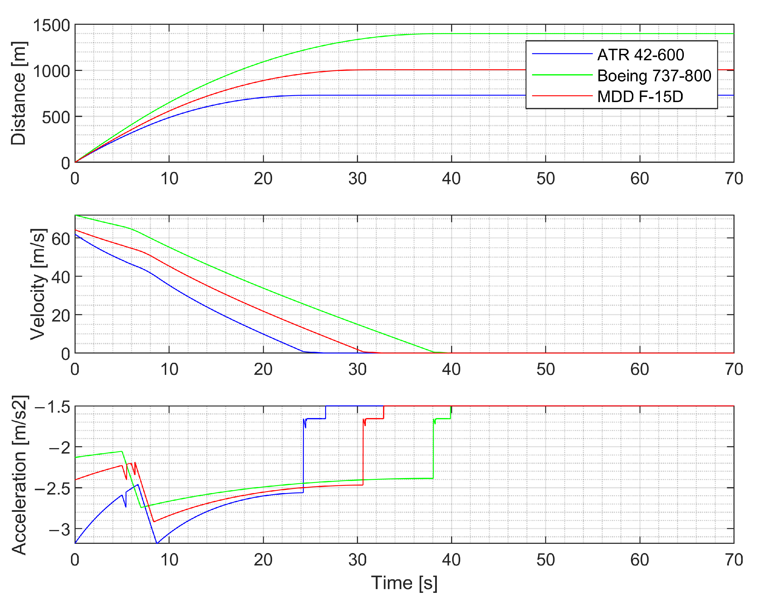
Finally, by looking at Figure 9, the kinematic behavior of the aircraft can be confirmed. In particular, the landing distances of the three aircraft are reported, alongside the longitudinal speed and acceleration characteristics. In the former, an almost linear trend can be noticed, which replicates the typical landing behavior [26]. In the latter, a sudden spike in deceleration can be seen at around 5 s, which corresponds to the start of the braking action.

4.2. Vertical Dynamics

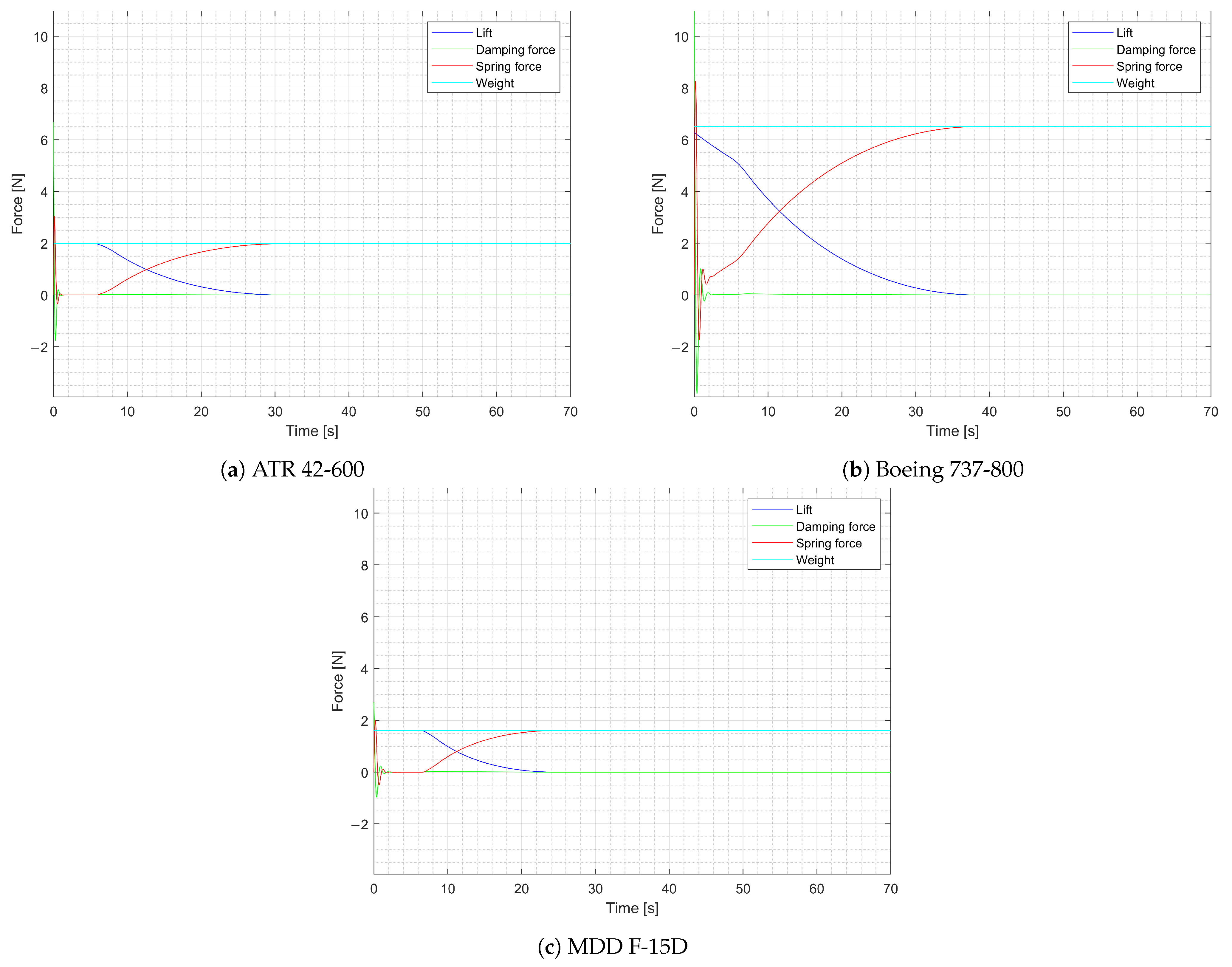
Next, alongside the longitudinal dynamics, the vertical dynamics curves can be plotted, which can be seen in Figure 10. Here, we can confirm a constant value of the weight of the aircraft and, similarly to the aerodynamic resistance, the exponential behavior of the aerodynamic lift.

It can be noticed that during the first few seconds, the weight and lift forces were the same: this was due to an artificial imposition of these forces to be equal to each other so as to simulate an equilibrium in the vertical direction maintained by the pilot. It can also be noticed how the Boeing 737-800 tended to reach similar values of lift and spring forces quite later than the other two aircraft: this may be considered to be the cause of the harsher intervention of the antiskid logic discussed earlier. The other two curves reported are the reaction forces of the landing gear, i.e., the spring force, and the damping force. As expected, both had a sinusoidal behavior, and the spring force became equal to the weight force when the aircraft stood still, while the damping force reached a null value, together with the aerodynamic lift, when the longitudinal speed of the aircraft also became null.

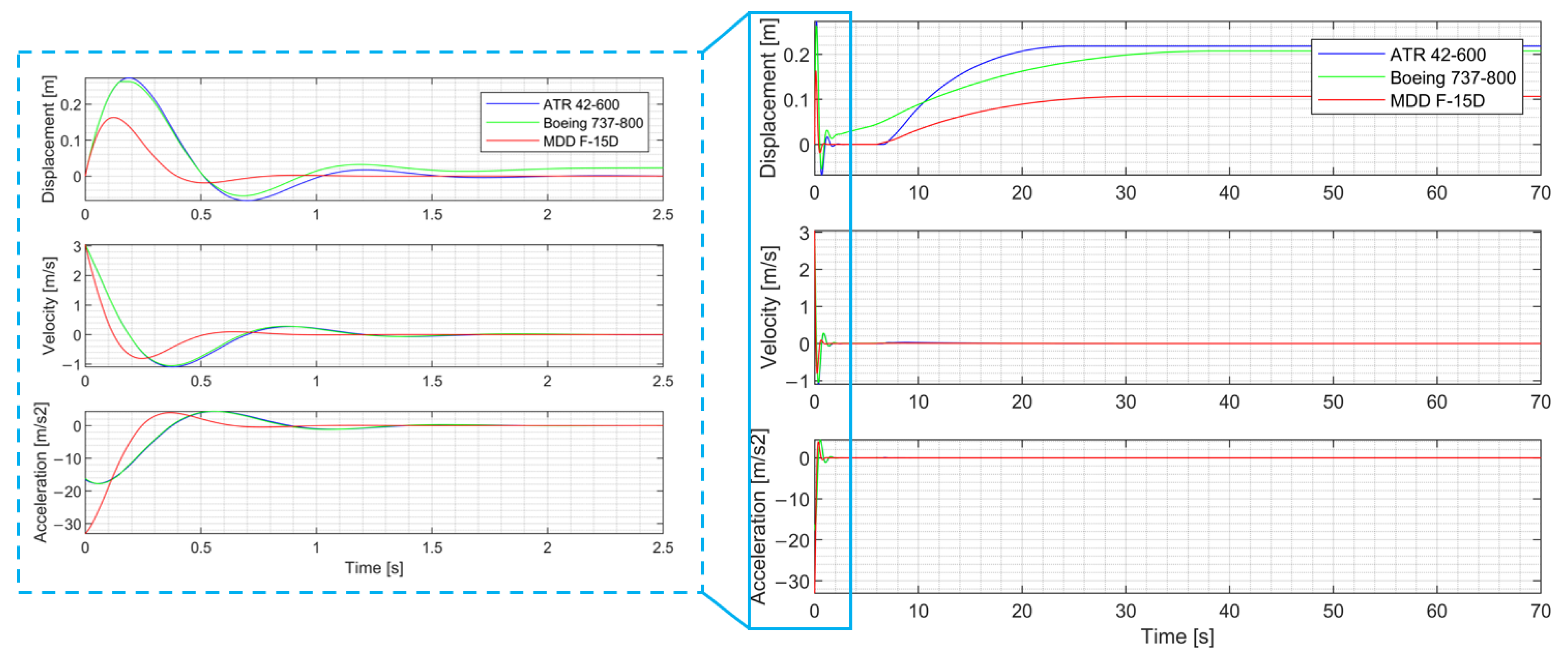
This relationship with the aircraft speed can be confirmed from Figure 11, where the kinematic behavior is reported. We can see that as soon as the aircraft touched the ground, a sudden vertical displacement srose due to the compression of the spring caused by the inertia of the aircraft, followed by a damped sinusoidal behavior, which was generated by the combination of the spring–damper system. Then, at standstill, the landing gear reached a steady-state compression due to the weight of the aircraft and the absence of aerodynamic lift. Such behavior is comparable to others found in the literature, thereby effectively simulating a mass spring–damper system [27,28].

4.3. Landing Gear

The last relevant results are regarding the behavior of the modeled components of the landing gear, more specifically the wheels and the brakes.

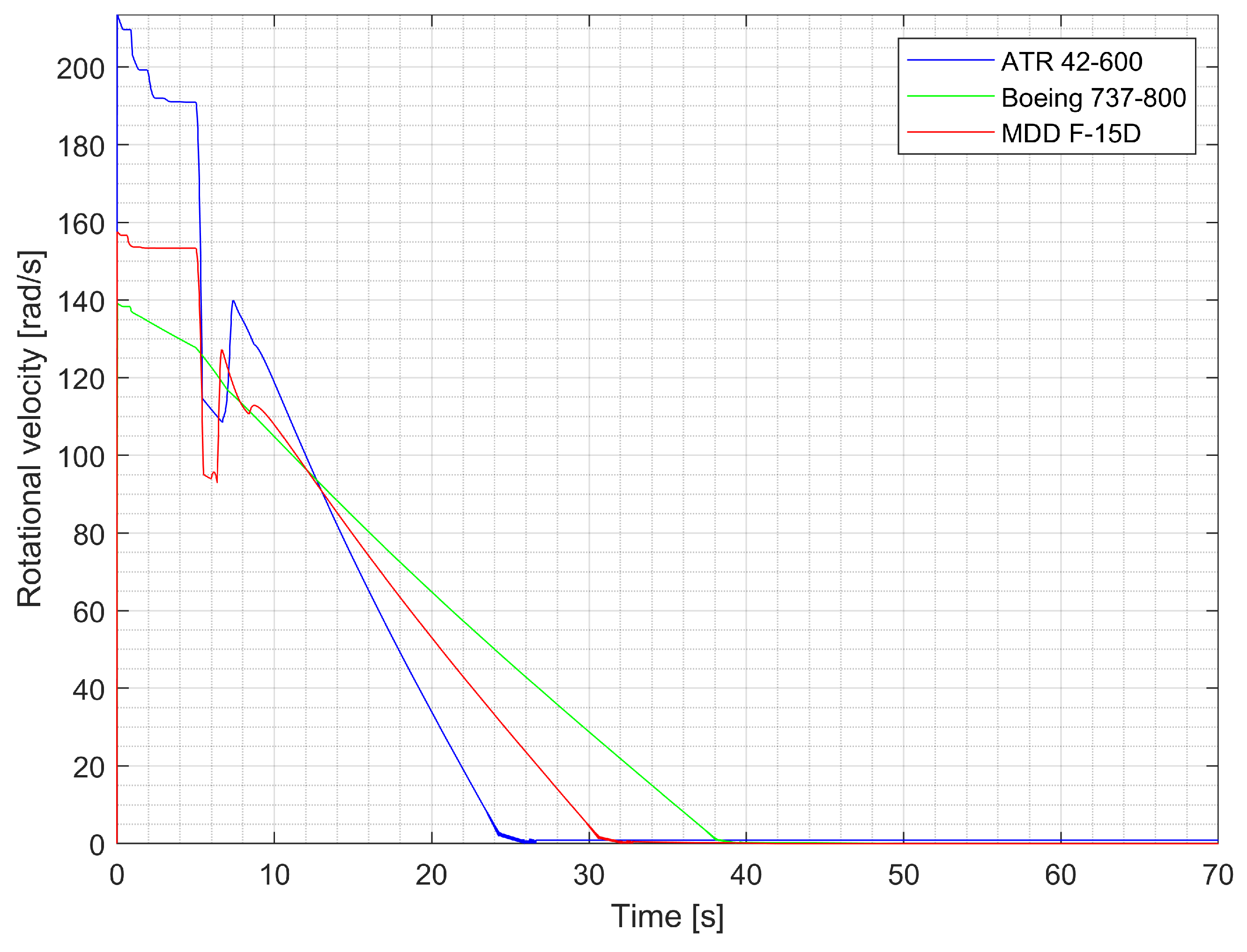
For what concerns the wheels, in Figure 12, the wheels’ rotational speeds are reported.

We can see that, as soon as the aircraft touched the ground, the wheels accelerated to a rotational speed that matches the longitudinal speed of the aircraft. At 5 s of simulation, the brakes were engaged, which caused a sudden reduction of the wheels’ speed. A few instants later, the slip coefficient reached a value of $-0.3$, which triggered the disengagement of the brakes, as explained earlier. It must be noted that in this phase, the aircraft is still in a transitional phase in terms of vertical displacement: therefore, the vertical reaction force is not sufficient to avoid wheel lock when the braking system is engaged. When the vertical force on the tires is sufficiently high, the wheels reach a sort of equilibrium, where their speeds match the aircraft speed, thus coming to a stop at the same time as the aircraft. A similar trend can be seen in other works found in the literature, including experimental tests showing a decrease in the wheel rotational speed with respect to the longitudinal aircraft speed when excessive braking force was applied [29,30,31]. It is noticeable that such phenomenon did not occur for the 737-800, since, as explained earlier, the mass of this aircraft made it possible to avoid the risk of wheel lock, thus not requiring the intervention of the antiskid system.

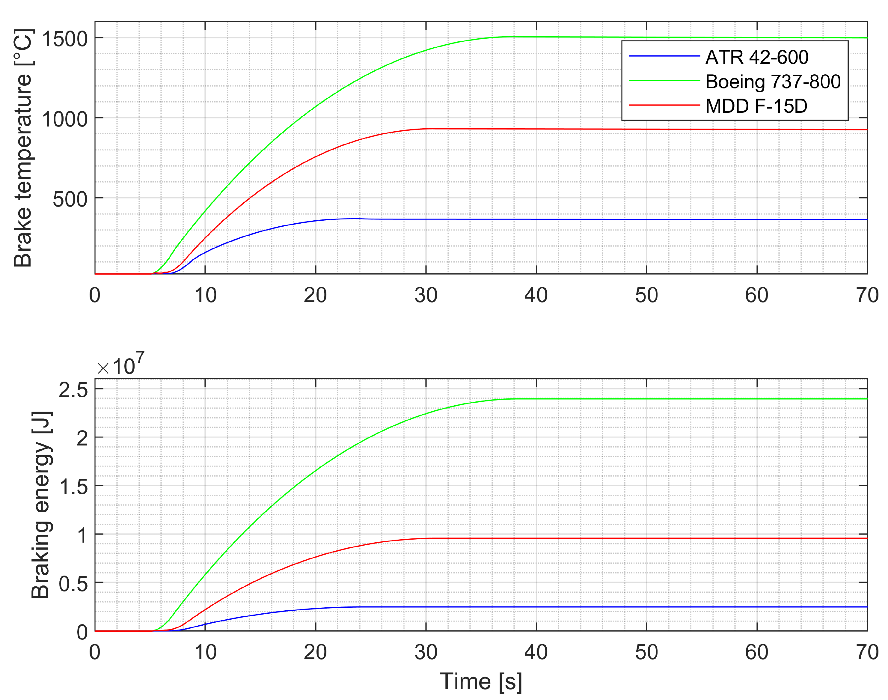
The other component considered in the landing gear are the brakes. In Figure 13, some relevant quantities are included.

First of all, the temperature reached by the brake is shown. As we can see, as the brakes were engaged at 5 s from landing, the temperatures started to increase. Such increases were slightly slower initially, due to the braking system control that, in the first braking phase, disengages the brakes a couple of times. When the brakes were fully engaged, the temperatures rose with a higher intensity until the braking action was stopped, as can also be seen in the literature [30]. It can be noticed that the Boeing 737-800 brakes reached temperatures that were much higher than the other two cases: this is most likely due to the much higher mass of this aircraft, thus requiring a larger amount of kinetic energy to be converted into thermal energy. The temperature curves behavior can be further confirmed from the curve of braking energy, which represents the mechanical energy converted into thermal energy by the brakes. It was obtained by integrating the braking power curve, reported in the same plot, and it clearly shows a similar trend to the temperature curve. This is to be expected, since there is a direct proportionality between the energy absorbed by a mass and its temperature, as was demonstrated by the experimental test performed by Meunier et al. [32].

5. Conclusions

From the study on the landing gear and the dynamics involved during landing, some relevant conclusions may be drawn. First of all, it is very clear that the design of the landing gear of an aircraft, whatever class or category it belongs to, is a very complex process that inevitably involves a large number of experts in various fields, thereby making it a very multidisciplinary system. Additionally, it can be considered to be a highly granular system, since it comprises numerous subsystems, such as the brakes and the wheels, each with its own specific function. It is therefore imperative to strive towards finding more and more efficient methods and techniques to properly design the said system, while all the while ensuring a high level of accuracy and reliability of the results from each analysis performed.

In this context, the current work presents a potential model-based design process, which makes it possible to quickly achieve a suitable configuration of the landing gear and verify its behavior during its expected operational scenario with a time-based dynamic model. In particular, the first section presented a complete mathematical workflow through which the characteristics of the individual subsystems may be estimated, starting with the main dimensions of the tires and wheels, based on data from real suppliers, which provided the data for the prediction of the wheel dynamic and kinematic behavior. Then, the braking system was sized to cope with the high mechanical and thermal stress deriving from the braking action during landing and to fit in the previously found wheel assembly solution.

Finally, the shock absorber was considered, thus finding suitable dimensions to make it possible to support the airframe and manage the impacts generated during landing. As the last step of the process, a dynamic model of the landing phase was introduced, which, based on the data obtained from the sizing script, made it possible to immediately verify the correct behavior of the landing gear and the interaction between its subsystems. In particular, it showed the temporal evolution of the dynamic behavior of the overall aircraft—both in the longitudinal and vertical directions—the thermal characteristics of the brakes, and how well the braking action was delivered, thereby taking into account the possible control logic that is employed and the rotational dynamics of the wheels, as well as showcasing the interaction between tires and runway. All these aspects can be confirmed through the results of the three aircraft test cases, thereby demonstrating the high flexibility of the process to size a wide variety of aircraft. Additionally, since the sizing model and dynamic model have been implemented in an inherently integrated digital environment, the need for complex manual computations, models setup, and data exchange between such models is completely eliminated.

As future developments, many improvements and additions may be performed on the models and the mathematical analysis. For instance, the sizing of all of the mechanical linkages composing the landing gear retraction mechanism may be added, alongside a multibody model, which makes it possible to quickly verify how the landing gear would retract and extend. Such a model could also be integrated with the prediction of the individual subsystems behavior to achieve a comprehensive dynamic analysis of the landing gear. Moreover, the subsystems that have been considered here could be further developed in order to obtain a more detailed analysis of their parameters, thereby even allowing for the automatic creation of a parametric CAD model, thus reducing the time required to set up complex simulations, such as through CFD or FEM analysis.