
Early Warning of Red Tide of Phaeocystis globosa Based on Phycocyanin Concentration Retrieval in Qinzhou Bay, China
Abstract
:
1. Introduction
2. Materials and Methods
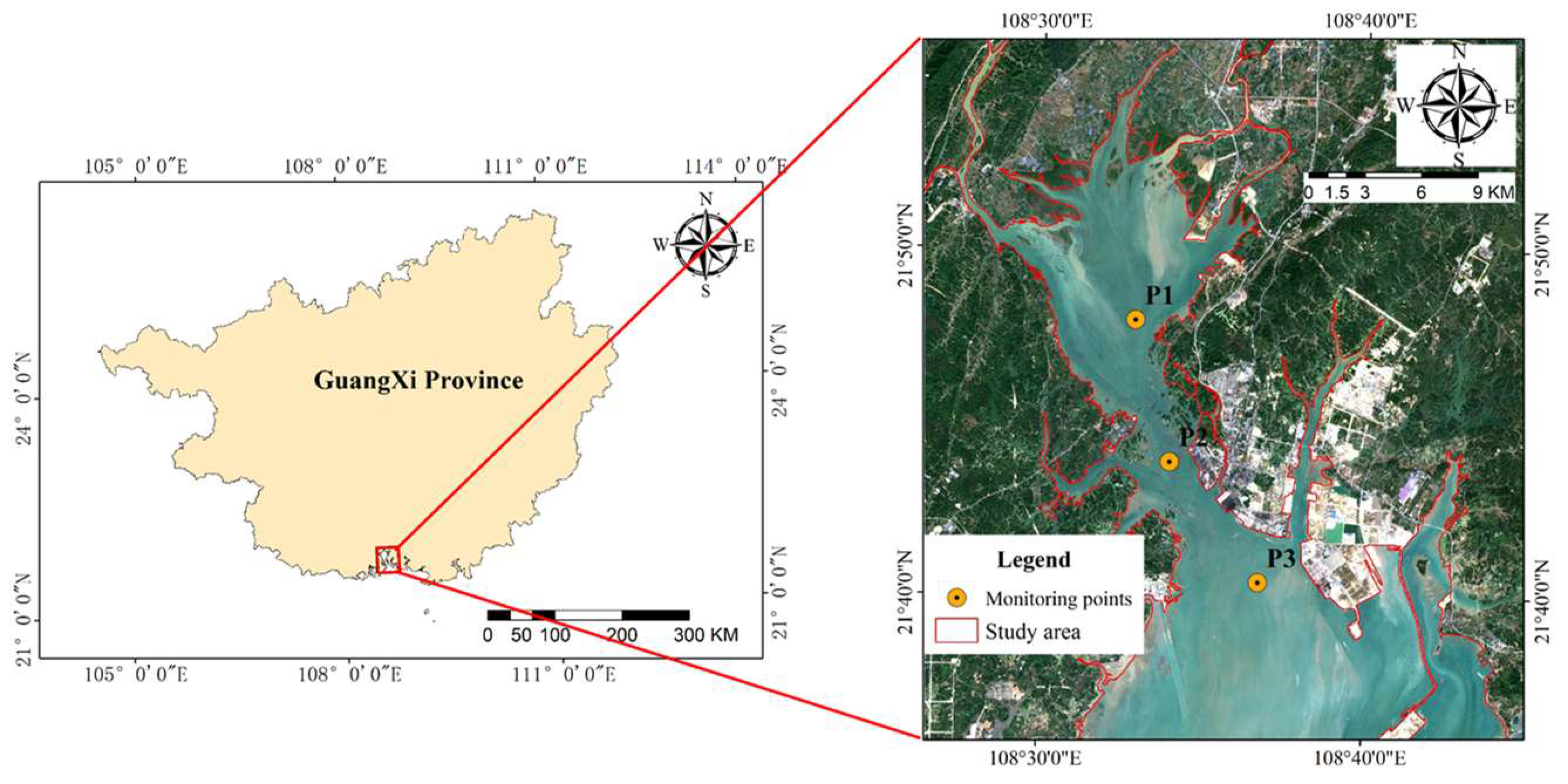
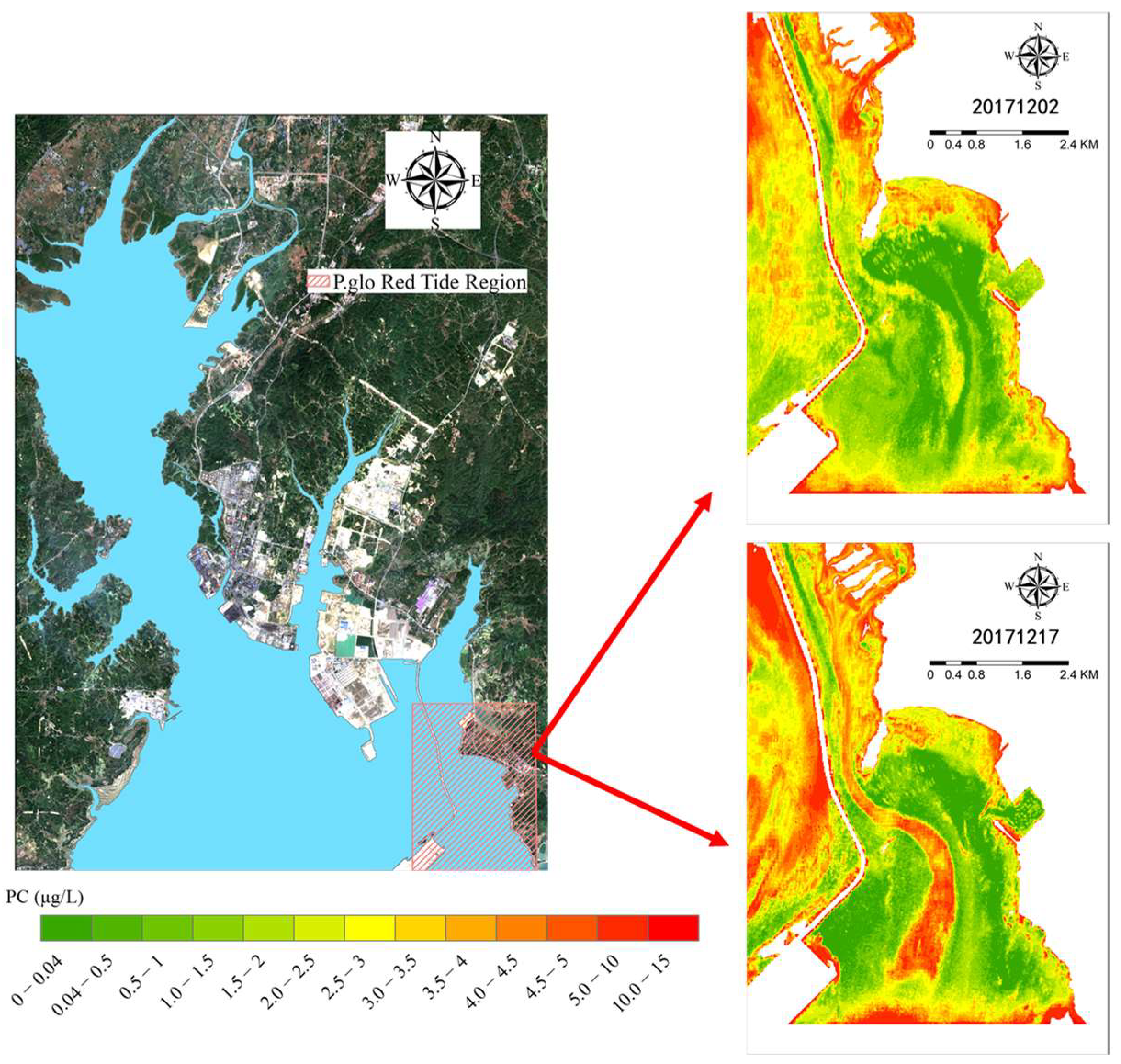
2.1. Study Area
2.2. Dataset
2.2.1. PC Concentration Monitoring Data
2.2.2. Remote Sensing Image Data
2.2.3. Other Data
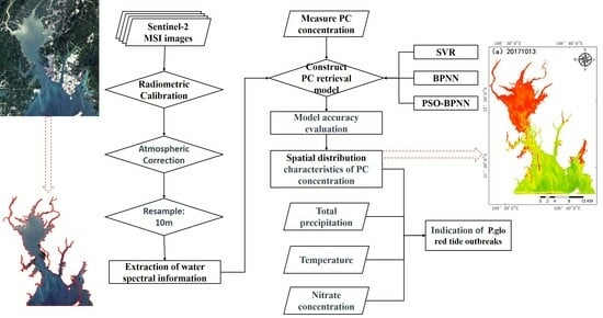
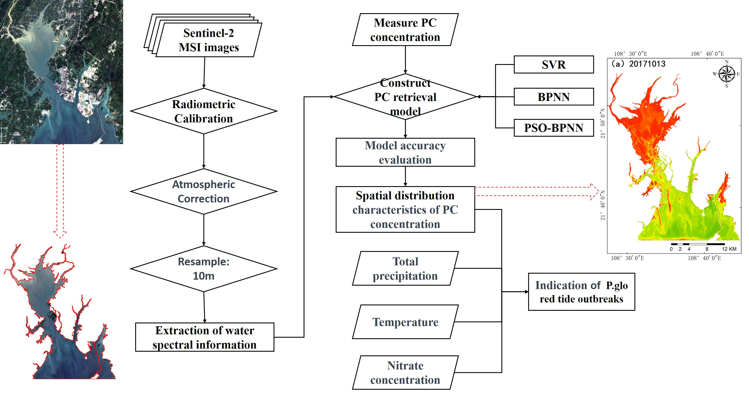
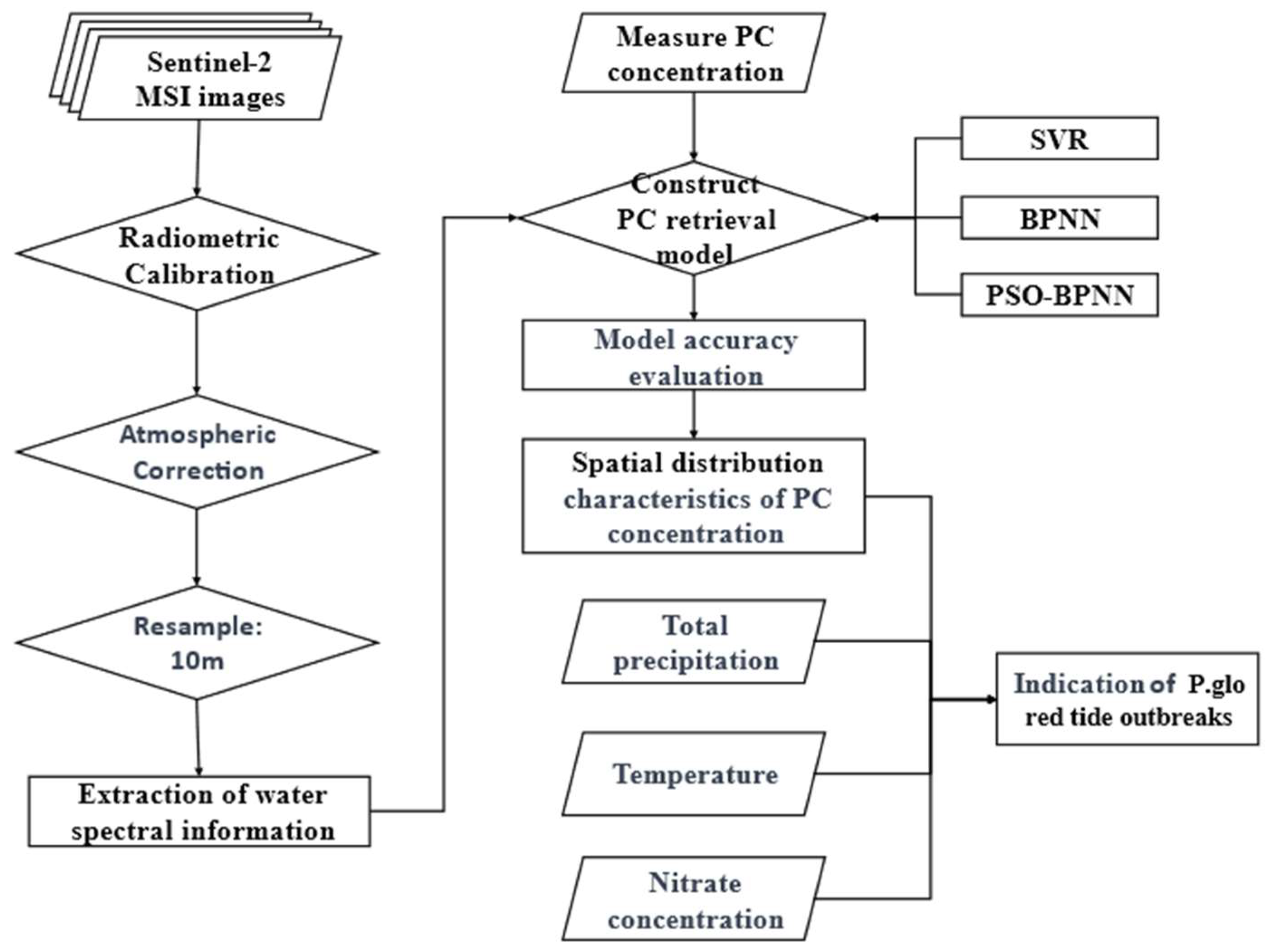
2.3. Methods
2.3.1. Image Preprocessing
2.3.2. Feature Preference
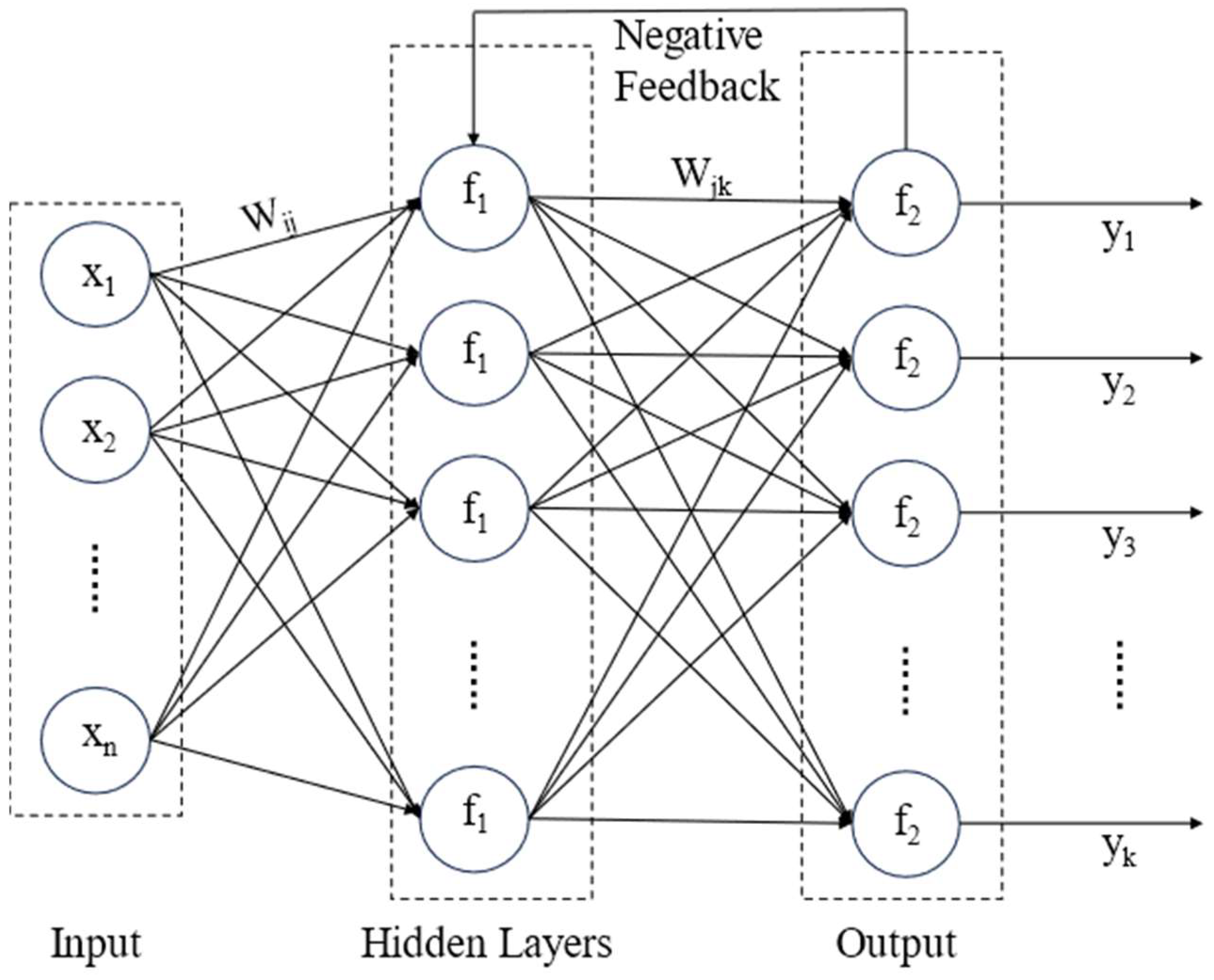
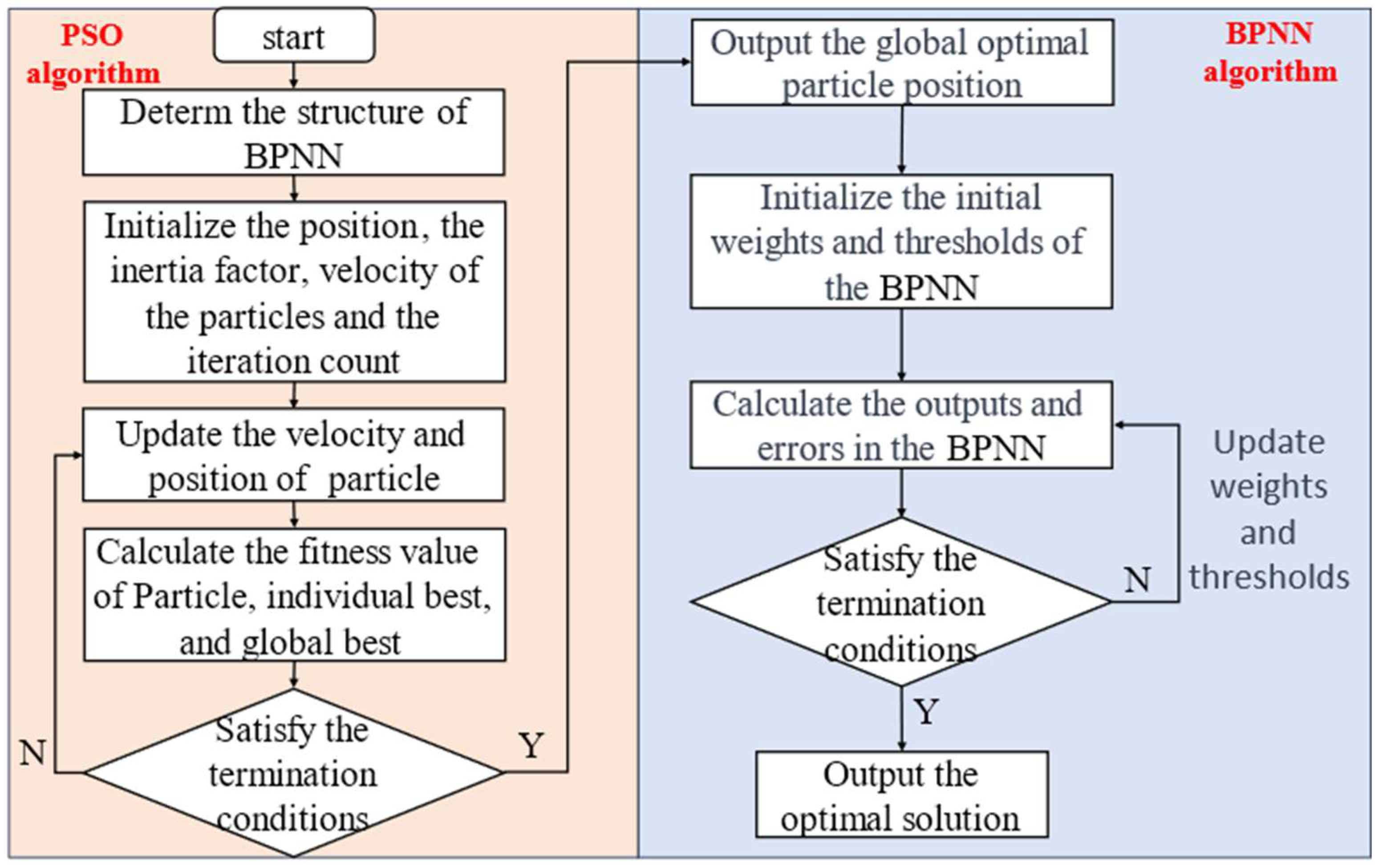
2.3.3. Model Building
2.3.4. Model Validation and Evaluation
3. Results
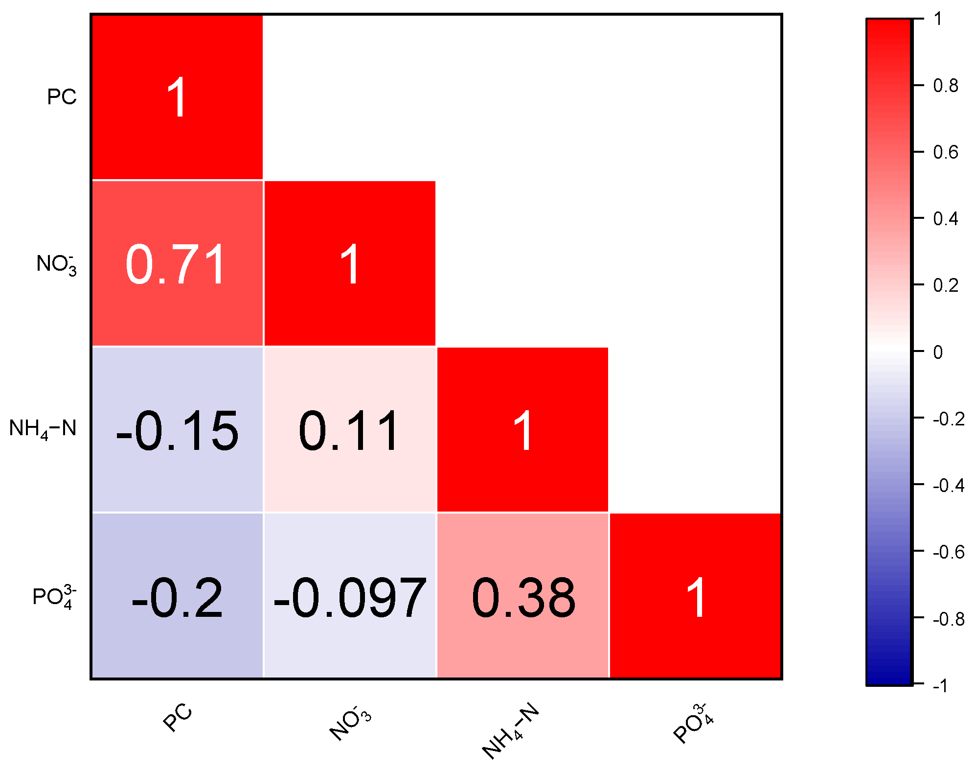
3.1. Results of Correlation Analysis
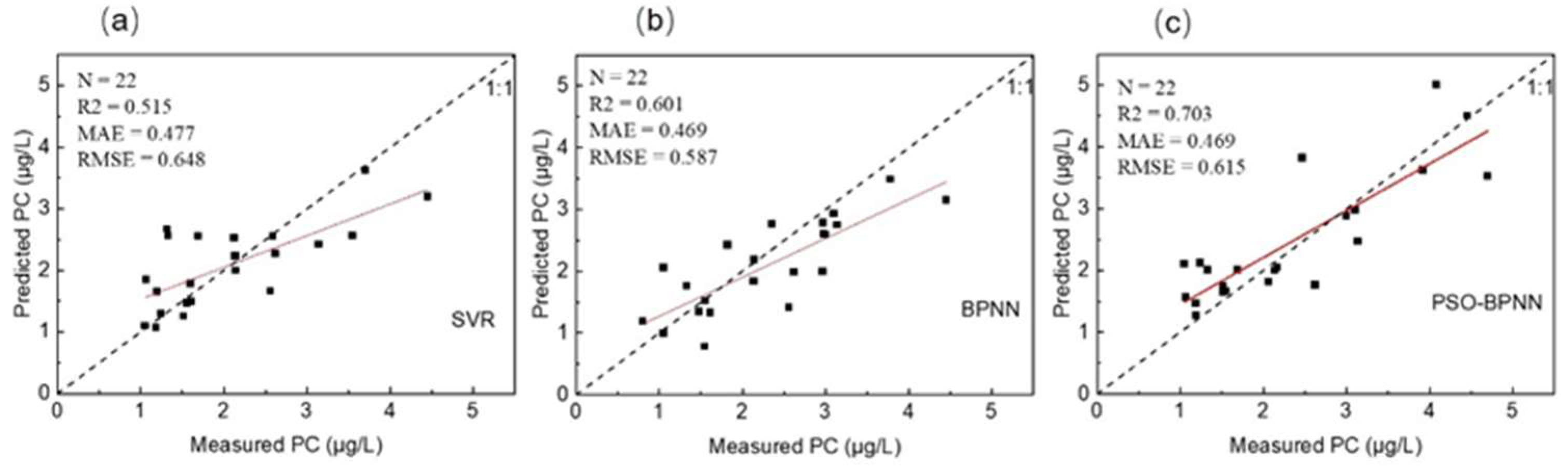
3.2. PC Retrieval Results and Validation
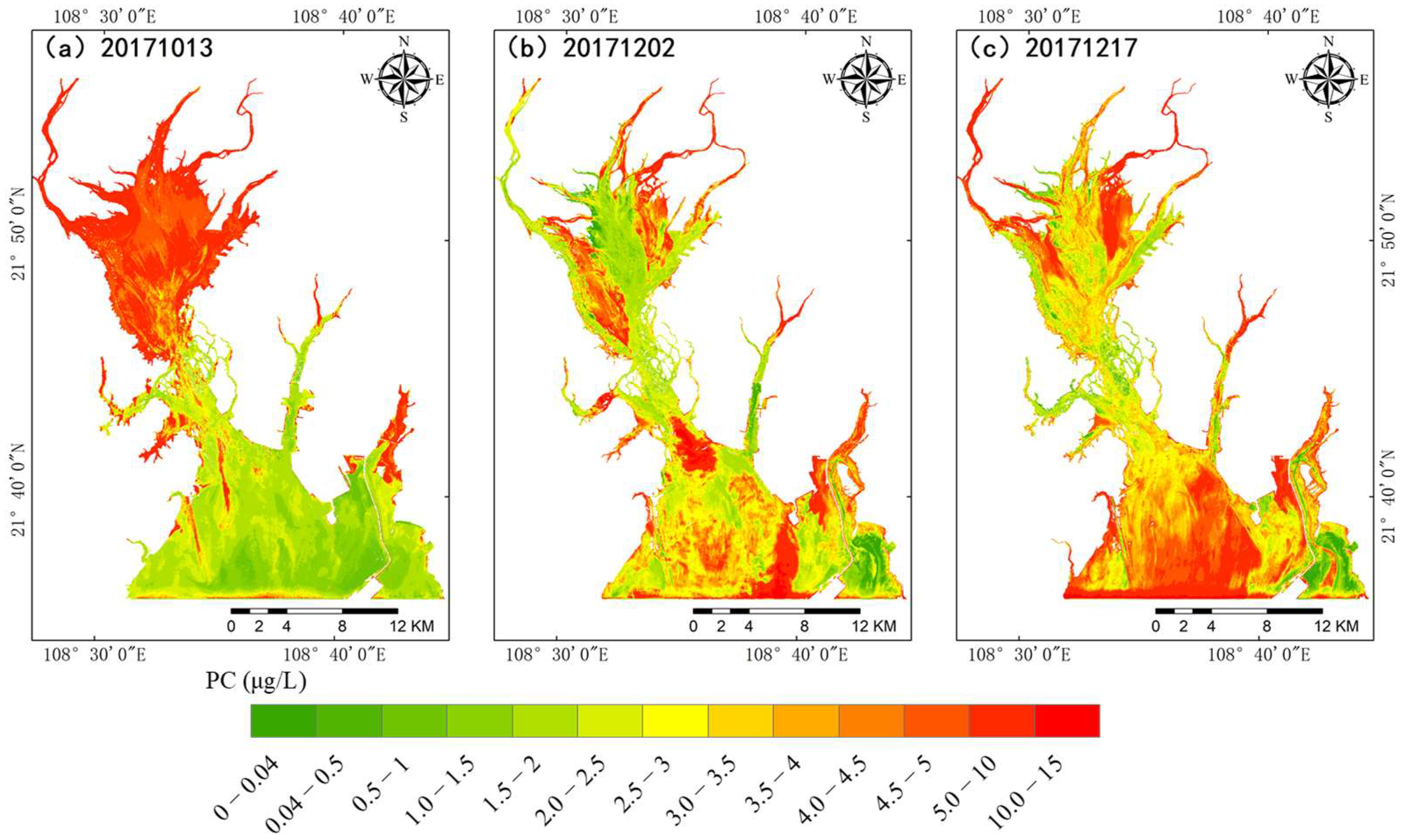
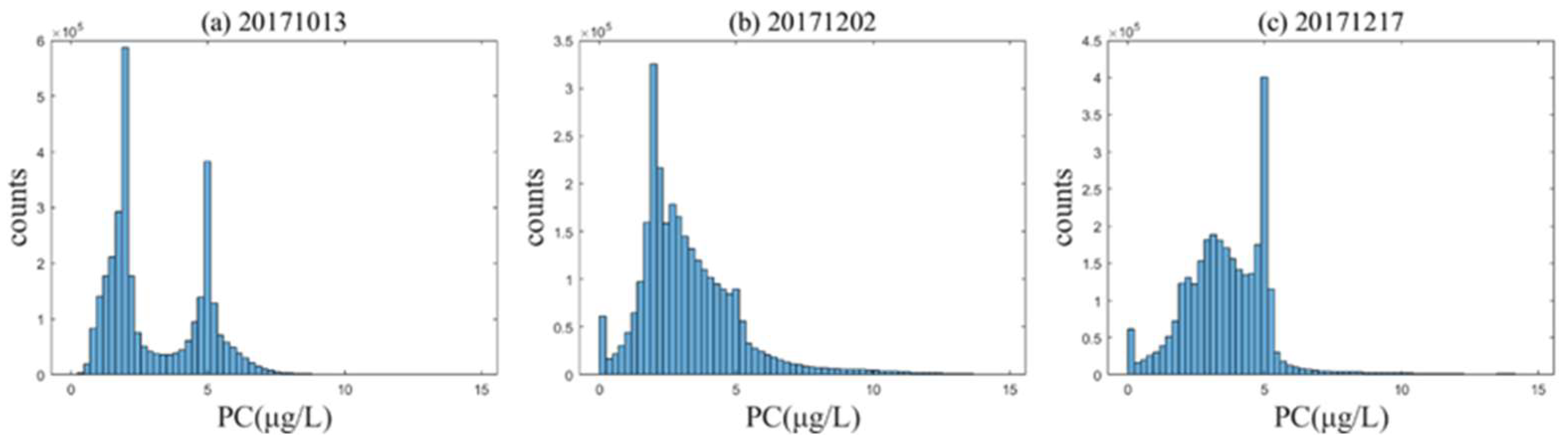
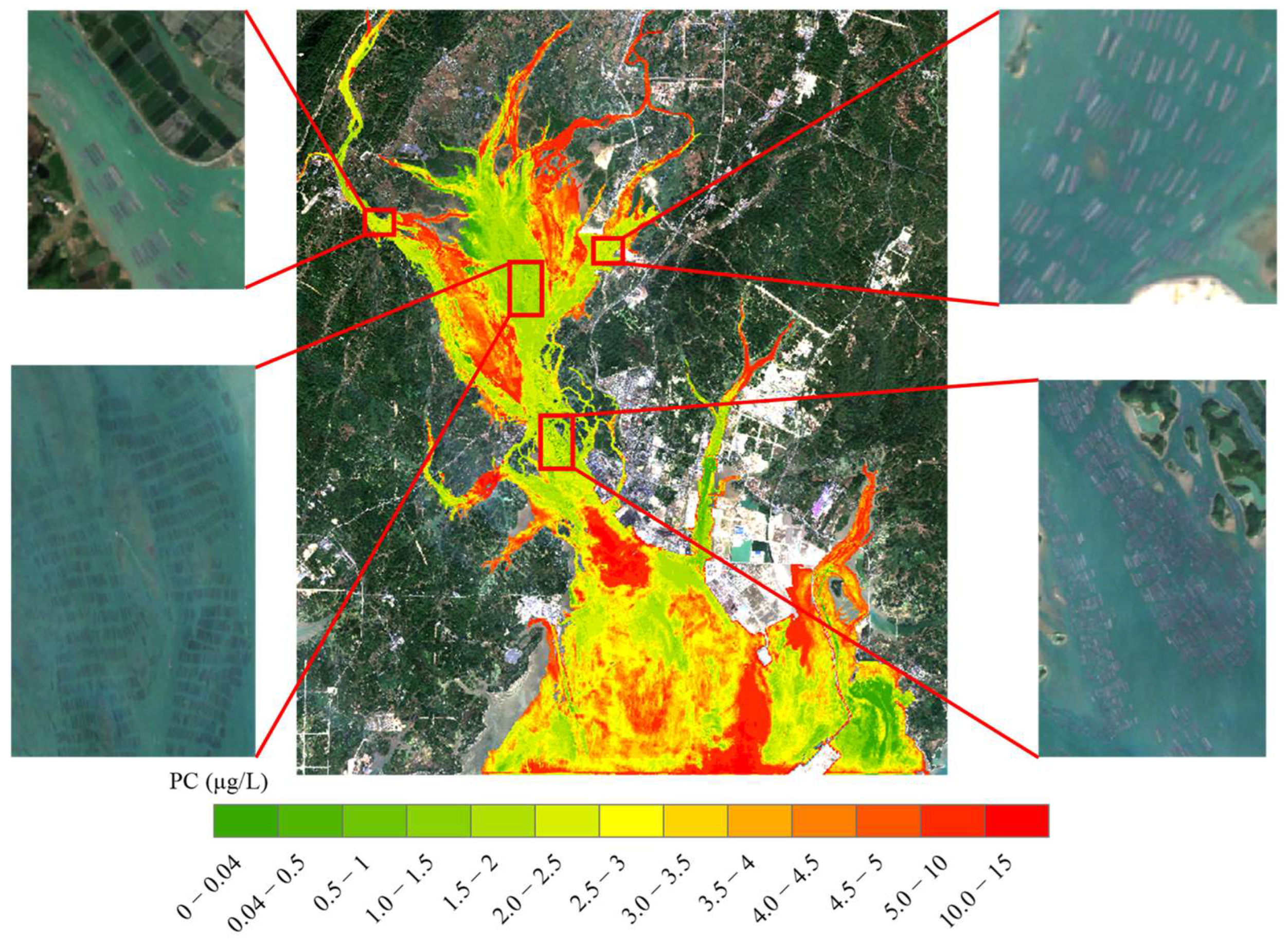
3.3. Characteristics of Spatial and Temporal Distribution of PC Concentration
4. Discussion
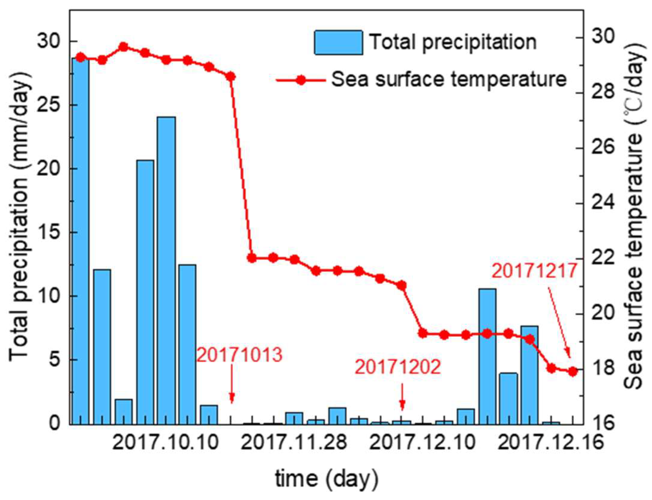
4.1. Effect of Total Precipitation and Temperature on PC Concentration
4.2. Effect of Nitrate on PC Concentration
4.3. Early Warning of P. glo Red Tide Outbreaks in Qinzhou Bay
5. Conclusions
Author Contributions
Funding
Institutional Review Board Statement
Informed Consent Statement
Data Availability Statement
Conflicts of Interest
Appendix A

| Bands | Resolution (m) | S2A Central Wavelength (nm) | S2B Central Wavelength (nm) |
|---|---|---|---|
| B1-Aerosols | 60 | 443.9 | 442.3 |
| B2-Blue | 10 | 496.6 | 492.1 |
| B3-Green | 10 | 560 | 559 |
| B4-Red | 10 | 664.5 | 665 |
| B5-Red Edge 1 | 20 | 703.9 | 703.8 |
| B6-Red Edge 2 | 20 | 740.2 | 739.1 |
| B7-Red Edge 3 | 20 | 782.5 | 779.7 |
| B8-NIR | 10 | 835.1 | 833 |
| B8A-Red Edge 4 | 20 | 864.8 | 864 |
| B9-Water vapor | 60 | 945 | 943.2 |
| B10-SWIR/Cirrus | 60 | 1375.5 | 1376.9 |
| B11-SWIR 1 | 20 | 1613.7 | 1610.4 |
| B12-SWIR 2 | 20 | 2202.4 | 2185.7 |
| Monitoring Date | Image Date | Image Quality |
|---|---|---|
| 18 December 2015 | 18 December 2015 | No cloud |
| 2 November 2016 | 2 November 2016 | Less than 10% cloud |
| 13 October 2017 | 13 October 2017 | No cloud |
| 27 November 2017 | 27 November 2017 | Less than 10% cloud |
| 2 December 2017 | 2 December 2017 | No cloud |
| 17 December 2017 | 17 December 2017 | No cloud |
| 22 March 2018 | 22 March 2018 | No cloud |
| 3 October 2018 | 3 October 2018 | Less than 10% cloud |
| 2 November 2018 | 2 November 2018 | No cloud |
| 22 November 2018 | 22 November 2018 | No cloud |
| 17 December 2018 | 17 December 2018 | No cloud |
| 9 August 2019 | 9 August 2019 | No cloud |
| 23 September 2019 | 23 September 2019 | No cloud |
| 28 September 2019 | 28 September 2019 | No cloud |
| 13 October 2019 | 13 October 2019 | No cloud |
| 18 October 2019 | 18 October 2019 | No cloud |
| 7 November 2019 | 7 November 2019 | No cloud |
| 22 November 2019 | 22 November 2019 | No cloud |
| 2 December 2019 | 2 December 2019 | No cloud |
| 7 December 2019 | 7 December 2019 | No cloud |
| 12 December 2019 | 12 December 2019 | No cloud |
| 18 December 2015 | 18 December 2015 | No cloud |
| 2 November 2016 | 2 November 2016 | Less than 10% cloud |
| 13 October 2017 | 13 October 2017 | No cloud |
| Parameter | Value |
|---|---|
| Hidden layer | 1 |
| Neurons in hidden layer | 10 |
| Training epochs | 1000 |
| Training goal | 1 × 10⁻⁶ |
| Learning rate | 0.01 |
| Activation function | tansig and purelin |
| Training algorithm | Levenberg–Marquardt |
| Loss function | mse |
References
- Rousseau, V.; Chretiennot-Dinet, M.-J.; Jacobsen, A.; Verity, P.; Whipple, S. The Life Cycle of Phaeocystis: State of Knowledge and Presumptive Role in Ecology. Biogeochemistry 2007, 83, 29–47. [Google Scholar] [CrossRef]
- Wu, N.; Fu, S.; Song, X.; Tong, M.; Jiang, T. Stress Regulation of Photosynthetic System of Phaeocystis globosa and Their Hemolytic Activity. J. Oceanol. Limnol. 2022, 40, 2164–2177. [Google Scholar] [CrossRef]
- Stoner, O.; Economou, T.; Torres, R.; Ashton, I.; Brown, R. Quantifying Spatio-Temporal Risk of Harmful Algal Blooms and Their Impacts on Bivalve Shellfish Mariculture Using a Data-Driven Modelling Approach. Harmful Algae 2023, 121, 102363. [Google Scholar] [CrossRef] [PubMed]
- Xu, Y.; Zhang, T.; Zhou, J. Historical Occurrence of Algal Blooms in the Northern Beibu Gulf of China and Implications for Future Trends. Front. Microbiol. 2019, 10, 451. [Google Scholar] [CrossRef]
- Huang, T. Morphological Characteristics of Colony for Phaeocystis globosa and the Influences of Light and Calcium Ion on Formation and Cell Distribution of Colony. Master’s Thesis, Jinan University, Guangzhou, China, 2012. [Google Scholar]
- Xu, M. The Key Influencing Factors in Solitary Cell and Colony Stages of Phaeocystis globosa in Beibu Gulf. Ph.D. Thesis, Guangxi University, Nanning, China, 2022. [Google Scholar]
- Qi, Y.; Shen, P.; Wang, Y. Taxonomy and lifecycle of genus Phaeocystis (prymnesiophyceae). J. Trop. Subtrop. Bot. 2001, 9, 174–184. [Google Scholar]
- Zhang, S.-F.; Han, B.-B.; Shi, R.-J.; Wu, F.-X.; Rao, Y.-Y.; Dai, M.; Huang, H.-H. Quantitative Proteomic Analysis Reveals the Key Molecular Events Driving Phaeocystis Globosa Bloom and Dissipation. Int. J. Mol. Sci. 2022, 23, 12668. [Google Scholar] [CrossRef]
- Qin, X.; Lai, J.; Chen, B.; Jinag, F.; Xu, M. Molecular Identification of Phaeocystis from Beibu Gulf Based on 18S rDNA Sequences. J. Trop. Subtrop. Bot. 2016, 24, 176–181. [Google Scholar]
- Zhao, Y.; Yu, R.; Zhang, Q.; Kong, F.; Kang, Z.; Cao, Z.; Geng, H.; Guo, W.; Zhou, M. Relationship between seasonal variation of pico-and nano-phytoplankton assemblages and Phaeocystis red tides in Beibu Gulf. Oceanol. Limnol. Sin. 2019, 50, 590–600. [Google Scholar] [CrossRef]
- Scanlan, D.J.; West, N.J. Molecular Ecology of the Marine Cyanobacterial Genera Prochlorococcus and Synechococcus. FEMS Microbiol. Ecol. 2002, 40, 1–12. [Google Scholar] [CrossRef]
- Yu, T.; Li, J.; Yang, Y.; Qi, L.; Chen, B.; Zhao, F.; Bao, Q.; Wu, J. Codon Usage Patterns and Adaptive Evolution of Marine Unicellular Cyanobacteria Synechococcus and Prochlorococcus. Mol. Phylogenetics Evol. 2012, 62, 206–213. [Google Scholar] [CrossRef]
- Lin, J.-Y.; Tan, S.; Yi, Y.-C.; Hsiang, C.-C.; Chang, C.-H.; Chen, C.-Y.; Chang, J.-S.; Ng, I.-S. High-Level Production and Extraction of C-Phycocyanin from Cyanobacteria Synechococcus Sp. PCC7002 for Antioxidation, Antibacterial and Lead Adsorption. Environ. Res. 2022, 206, 112283. [Google Scholar] [CrossRef] [PubMed]
- Glazer, A.N.; Fang, S. Chromophore Content of Blue-Green Algal Phycobiliproteins. J. Biol. Chem. 1973, 248, 659–662. [Google Scholar] [CrossRef] [PubMed]
- Simis, S.G.H.; Ruiz-Verdu, A.; Antonio Dominguez-Gomez, J.; Pena-Martinez, R.; Peters, S.W.M.; Gons, H.J. Influence of Phytoplankton Pigment Composition on Remote Sensing of Cyanobacterial Biomass. Remote Sens. Environ. 2007, 106, 414–427. [Google Scholar] [CrossRef]
- Qi, L.; Hu, C.; Duan, H.; Cannizzaro, J.; Ma, R. A Novel MERIS Algorithm to Derive Cyanobacterial Phycocyanin Pigment Concentrations in a Eutrophic Lake: Theoretical Basis and Practical Considerations. Remote Sens. Environ. 2014, 154, 298–317. [Google Scholar] [CrossRef]
- Hunter, P.D.; Tyler, A.N.; Carvalho, L.; Codd, G.A.; Maberly, S.C. Hyperspectral Remote Sensing of Cyanobacterial Pigments as Indicators for Cell Populations and Toxins in Eutrophic Lakes. Remote Sens. Environ. 2010, 114, 2705–2718. [Google Scholar] [CrossRef]
- Gitelson, A.A.; Gritz, Y.; Merzlyak, M.N. Relationships between Leaf Chlorophyll Content and Spectral Reflectance and Algorithms for Non-Destructive Chlorophyll Assessment in Higher Plant Leaves. J. Plant Physiol. 2003, 160, 271–282. [Google Scholar] [CrossRef]
- Mishra, S.; Mishra, D.R. A Novel Remote Sensing Algorithm to Quantify Phycocyanin in Cyanobacterial Algal Blooms. Environ. Res. Lett. 2014, 9, 114003. [Google Scholar] [CrossRef]
- Wang, Z.; Wang, J.; Yan, S.; Cui, Y.; Wang, H. Annual dynamic remote sensing monitoring of phycocyanin concentration in Lake Chaohu based on Sentinel-3 OLCI images. J. Lake Sci. 2022, 34, 391–403. [Google Scholar] [CrossRef]
- Wang, J.; Wang, Z.; Cui, Y.; Yan, S. Dynamic Monitoring of Phycocyanin Concentration in Chaohu Lake of China Using Sentinel-3 Images and Its Indication of Cyanobacterial Blooms. Ecol. Indic. 2022, 143, 109340. [Google Scholar] [CrossRef]
- Song, K.; Li, L.; Li, S.; Tedesco, L.; Hall, B.; Li, Z. Hyperspectral Retrieval of Phycocyanin in Potable Water Sources Using Genetic Algorithm-Partial Least Squares (GA-PLS) Modeling. Int. J. Appl. Earth Obs. Geoinf. 2012, 18, 368–385. [Google Scholar] [CrossRef]
- Pyo, J.; Duan, H.; Baek, S.; Kim, M.S.; Jeon, T.; Kwon, Y.S.; Lee, H.; Cho, K.H. A Convolutional Neural Network Regression for Quantifying Cyanobacteria Using Hyperspectral Imagery. Remote Sens. Environ. 2019, 233, 111350. [Google Scholar] [CrossRef]
- Beck, R.; Xu, M.; Zhan, S.; Johansen, R.; Liu, H.; Tong, S.; Yang, B.; Shu, S.; Wu, Q.; Wang, S.; et al. Comparison of Satellite Reflectance Algorithms for Estimating Turbidity and Cyanobacterial Concentrations in Productive Freshwaters Using Hyperspectral Aircraft Imagery and Dense Coincident Surface Observations. J. Great Lakes Res. 2019, 45, 413–433. [Google Scholar] [CrossRef] [PubMed]
- Wang, Y.-H.; Tang, L.-Q.; Wang, C.-H.; Liu, C.-J.; Dong, Z.-D. Combined Effects of Channel Dredging, Land Reclamation and Long-Range Jetties upon the Long-Term Evolution of Channel-Shoal System in Qinzhou Bay, SW China. Ocean Eng. 2014, 91, 340–349. [Google Scholar] [CrossRef]
- Song, D.; Bao, X.; Zhu, X. Three-dimensional numerical simulation of tidal current in Qinzhou Bay. J. Trop. Oceanogr. 2009, 28, 7–14. [Google Scholar]
- Gao, B.C. NDWI—A Normalized Difference Water Index for Remote Sensing of Vegetation Liquid Water from Space. Remote Sens. Environ. 1996, 58, 257–266. [Google Scholar] [CrossRef]
- Yue, H.; Li, Y.; Qian, J.; Liu, Y. A New Accuracy Evaluation Method for Water Body Extraction. Int. J. Remote Sens. 2020, 41, 7311–7342. [Google Scholar] [CrossRef]
- Yuan, C.; Sun, X.; Wu, Q.M.J. Difference Co-Occurrence Matrix Using BP Neural Network for Fingerprint Liveness Detection. Soft Comput. 2019, 23, 5157–5169. [Google Scholar] [CrossRef]
- Lyu, J.; Zhang, J. BP Neural Network Prediction Model for Suicide Attempt among Chinese Rural Residents. J. Affect. Disord. 2019, 246, 465–473. [Google Scholar] [CrossRef]
- Wang, L.; Zeng, Y.; Chen, T. Back Propagation Neural Network with Adaptive Differential Evolution Algorithm for Time Series Forecasting. Expert Syst. Appl. 2015, 42, 855–863. [Google Scholar] [CrossRef]
- Wu, Y.; Wu, D.; Fei, M.; Sorensen, H.; Ren, Y.; Mou, J. Application of GA-BPNN on Estimating the Flow Rate of a Centrifugal Pump. Eng. Appl. Artif. Intell. 2023, 119, 105738. [Google Scholar] [CrossRef]
- Zhang, L.; Sun, Z.; Zhang, C.; Dong, F.; Wei, P. Numerical Investigation of the Dynamic Responses of Long-Span Bridges with Consideration of the Random Traffic Flow Based on the Intelligent ACO-BPNN Model. IEEE Access 2018, 6, 28520–28529. [Google Scholar] [CrossRef]
- Ling, X.; Xu, L.; Liang, R.; Guo, K.; Cui, B.; Yue, S. Study on internal corrosion rate of oil pipeline based on improved PSO–BPNN. J. Saf. Sci. Technol. 2019, 15, 63–68. [Google Scholar] [CrossRef]
- Shi, Y.; Eberhart, R.C. Empirical Study of Particle Swarm Optimization. In Proceedings of the 1999 Congress on Evolutionary Computation-CEC99 (Cat. No. 99TH8406), Washington, DC, USA, 6–9 July 1999; IEEE: Piscataway, NJ, USA, 1999; Volume 3, pp. 1945–1950. [Google Scholar]
- Song, Y.; Zhang, F.; Liu, C. The Risk of Block Chain Financial Market Based on Particle Swarm Optimization. J. Comput. Appl. Math. 2020, 370, 112667. [Google Scholar] [CrossRef]
- Li, L.; Li, L.; Song, K. Remote Sensing of Freshwater Cyanobacteria: An Extended IOP Inversion Model of Inland Waters (IIMIW) for Partitioning Absorption Coefficient and Estimating Phycocyanin. Remote Sens. Environ. 2015, 157, 9–23. [Google Scholar] [CrossRef]
- Beck, R.; Xu, M.; Zhan, S.; Liu, H.; Johansen, R.A.; Tong, S.; Yang, B.; Shu, S.; Wu, Q.; Wang, S.; et al. Comparison of Satellite Reflectance Algorithms for Estimating Phycocyanin Values and Cyanobacterial Total Biovolume in a Temperate Reservoir Using Coincident Hyperspectral Aircraft Imagery and Dense Coincident Surface Observations. Remote Sens. 2017, 9, 538. [Google Scholar] [CrossRef]
- Riddick, C.A.L.; Hunter, P.D.; Dominguez Gomez, J.A.; Martinez-Vicente, V.; Presing, M.; Horvath, H.; Kovacs, A.W.; Voros, L.; Zsigmond, E.; Tyler, A.N. Optimal Cyanobacterial Pigment Retrieval from Ocean Colour Sensors in a Highly Turbid, Optically Complex Lake. Remote Sens. 2019, 11, 1613. [Google Scholar] [CrossRef]
- Tian, S.; Huang, J.; Li, G. On the noise sensitivity of ε-support vector regression. Fire Control Command. Control 2013, 38, 130–132+140. [Google Scholar]
- Avila-Poveda, O.H.; Torres-Arino, A.; Giron-Cruz, D.A.; Cuevas-Aguirre, A. Evidence for Accumulation of Synechococcus elongatus (Cyanobacteria: Cyanophyceae) in the Tissues of the Oyster Crassostrea gigas (Mollusca: Bivalvia). Tissue Cell 2014, 46, 379–387. [Google Scholar] [CrossRef]
- Straquadine, N.R.W.; Kudela, R.M.; Gobler, C.J. Hepatotoxic Shellfish Poisoning: Accumulation of Microcystins in Eastern Oysters (Crassostrea virginica) and Asian Clams (Corbicula fluminea) Exposed to Wild and Cultured Populations of the Harmful Cyanobacteria, Microcystis. Harmful Algae 2022, 115, 102236. [Google Scholar] [CrossRef]
- Lv, X. The Key Effect of Nitrate on Phaeocystis globosa Booms in the Beibu Gulf. Ph.D. Thesis, University of Chinese Academy of Sciences (Oceanography Researcher, Chinese Academy of Sciences), Qingdao, China, 2020. [Google Scholar]
- Zhang, D. The Influence Factors for Spatio-Temporal Changes of Nutrients and the Quantitative Reduction of Terrestrial TDN in Qinzhou Bay. Ph.D. Thesis, Guangxi University, Nanning, China, 2020. [Google Scholar]
- Lv, H.; Zhang, S.; Song, D.; Bao, X. The cummulative effect of land reclamation on hydrodynamics in Qinzhou Bay. Oceanol. Limnol. Sin. 2021, 52, 823–833. [Google Scholar]
- Xu, Y.; Liao, R.; Su, J.; Gong, L. The content and pollution evaluation of six heavy metals in surface water and plankton in the eastern area of Qinzhou Bay. Oceanol. Limnol. Sin. 2017, 48, 960–969. [Google Scholar]


| No. | Time | Descriptions |
|---|---|---|
| 1 | January 2015~March 2015 | Wide-ranging and long-lasting impacts |
| 2 | November 2015~December 2015 | Area not available |
| 3 | December 2016 | Area not available |
| 4 | January 2017~March 2017 | Dull water color and unknown size |
| 5 | November 2017~December 2017 | Area not available |
| 6 | January 2018 | Concentrations reach high levels |
| 7 | January 2019~February 2019 | Area not available |
| Monitor Point | Longitude | Latitude |
|---|---|---|
| S1 | 108.5483 | 21.7992 |
| S2 | 108.5667 | 21.7312 |
| S3 | 108.6128 | 21.6737 |
| Water Quality Parameters | Maximum | Minimum | Mean | Median | Standard Deviation | N |
|---|---|---|---|---|---|---|
| S1-PC (μg/L) | 4.855 | 0.799 | 2.131 | 1.672 | 1.208 | 20 |
| S2-PC (μg/L) | 4.450 | 1.050 | 2.169 | 2.163 | 0.891 | 18 |
| S3-PC (μg/L) | 4.695 | 1.190 | 2.573 | 2.170 | 1.119 | 17 |
| Total-PC (μg/L) | 4.855 | 0.799 | 2.280 | 2.125 | 1.083 | 55 |
| Band/Spectral Index | R | Band/Spectral Index | R | Band/Spectral Index | R |
|---|---|---|---|---|---|
| B1 | 0.633 ** | B2/B1 | −0.222 | NDVI | −0.400 ** |
| B2 | 0.500 ** | B2/B3 | −0.422 | NDWI | 0.071 |
| B3 | 0.640 ** | B2/B4 | −0.538 | MNDWI | 0.146 |
| B4 | 0.646 ** | B2/B5 | −0.346 | (B2 + B8)/B4 | −0.651 ** |
| B5 | 0.482 ** | B4/B3 | 0.500 | (B3 + B8)/B4 | −0.644 ** |
| B6 | 0.206 | B4/B8 | 0.401 | B6/B1 + B3/B4 | −0.615 ** |
| B7 | 0.140 | B5/B6 | 0.423 | B6/B1 + B2/B4 | −0.630 ** |
| B8 | 0.221 | B5/B7 | 0.503 | B7/B1 + B3/B4 | −0.615 ** |
| Model | Train | Test | ||||
|---|---|---|---|---|---|---|
| MAE | RMSE | R2 | MAE | RMSE | R2 | |
| SVR | 0.383 | 0.580 | 0.686 | 0.600 | 0.728 | 0.505 |
| BPNN | 0.408 | 0.603 | 0.730 | 0.469 | 0.587 | 0.601 |
| PSO-BPNN | 0.376 | 0.582 | 0.782 | 0.469 | 0.615 | 0.703 |
Disclaimer/Publisher’s Note: The statements, opinions and data contained in all publications are solely those of the individual author(s) and contributor(s) and not of MDPI and/or the editor(s). MDPI and/or the editor(s) disclaim responsibility for any injury to people or property resulting from any ideas, methods, instructions or products referred to in the content. |
© 2023 by the authors. Licensee MDPI, Basel, Switzerland. This article is an open access article distributed under the terms and conditions of the Creative Commons Attribution (CC BY) license (https://creativecommons.org/licenses/by/4.0/).
Share and Cite
Liu, Y.; Yao, H.; Chen, H.; Wang, M.; Huang, Z.; Zhong, W. Early Warning of Red Tide of Phaeocystis globosa Based on Phycocyanin Concentration Retrieval in Qinzhou Bay, China. Appl. Sci. 2023, 13, 11449. https://doi.org/10.3390/app132011449
Liu Y, Yao H, Chen H, Wang M, Huang Z, Zhong W. Early Warning of Red Tide of Phaeocystis globosa Based on Phycocyanin Concentration Retrieval in Qinzhou Bay, China. Applied Sciences. 2023; 13(20):11449. https://doi.org/10.3390/app132011449
Chicago/Turabian StyleLiu, Yin, Huanmei Yao, Huaquan Chen, Mengsi Wang, Zengshiqi Huang, and Weiping Zhong. 2023. "Early Warning of Red Tide of Phaeocystis globosa Based on Phycocyanin Concentration Retrieval in Qinzhou Bay, China" Applied Sciences 13, no. 20: 11449. https://doi.org/10.3390/app132011449