Article

Quantitative Analysis of Biodiesel Adulterants Using Raman Spectroscopy Combined with Synergy Interval Partial Least Squares (siPLS) Algorithms

1
College of Chemistry and Chemical Engineering, Xi’an Shiyou University, Xi’an 710065, China
2
Key Laboratory of Synthetic and Natural Functional Molecule of the Ministry of Education, College of Chemistry & Materials Science, Northwest University, Xi’an 710127, China
*
Authors to whom correspondence should be addressed.
Appl. Sci. 2023, 13(20), 11306; https://doi.org/10.3390/app132011306
Submission received: 20 September 2023 / Revised: 8 October 2023 / Accepted: 12 October 2023 / Published: 14 October 2023
(This article belongs to the Special Issue Spectral Detection: Technologies and Applications)

Abstract

:
Biodiesel has emerged as an alternative to traditional fuels with the aim of reducing the impact on the environment. It is produced by the esterification of oleaginous seeds, animal fats, etc., with short-chain alcohols in an alkaline solution, which is one of the most commonly used methods. This increases the oxygen content (from the fatty acids) and promotes the fuel to burn faster and more efficiently. The accurate quantification of biodiesel is of paramount importance to the fuel market due to the possibility of adulteration, which can result in economic losses, engine performance issues and environmental concerns related to corrosion. In response to achieving this goal, in this work, synergy interval partial least squares (siPLS) algorithms in combination with Raman spectroscopy are used for the quantification of the biodiesel content. Different pretreatment methods are discussed to eliminate a large amount of redundant information of the original spectrum. The siPLS technique for extracting feature variables is then used to optimize the input variables after pretreatment, in order to enhance the predictive performance of the calibration model. Finally, the D1-MSC-siPLS calibration model is constructed based on the preprocessed spectra, the selected input variables and the optimized model parameters. Compared with the feature variable selection methods of interval partial least squares (iPLS) and backward interval partial least squares (biPLS), results elucidate that the D1-MSC-siPLS calibration model is superior to the D1-MSC-biPLS and the D1-MSC-iPLS in the quantitative analysis of adulterated biodiesel. The D1-MSC-siPLS calibration model demonstrates better predictive performance compared to the full spectrum PLS model, with the optimal determination coefficient of prediction (R2P) being 0.9899; the mean relative error of prediction (MREP) decreased from 9.51% to 6.31% and the root--mean-squared error of prediction (RMSEP) decreased from 0.1912% (v/v) to 0.1367% (v/v), respectively. The above results indicate that Raman spectroscopy combined with the D1-MSC-siPLS calibration model is a feasible method for the quantitative analysis of biodiesel in adulterated hybrid fuels.

1. Introduction

The increase in global greenhouse gas emissions and the scarcity of petroleum fuels have prompted a search for clean and sustainable alternative energy sources. One of these is biodiesel, which has become the main fuel for the transport industry in several countries [1,2]. Biodiesel is produced using the transesterification reactions of short-chain alcohols (methanol or ethanol) with oil-containing seeds, animal fats or recycled cooking oils [3,4], catalyzed by acids, bases and enzymes. Acid and base catalysis can be homogeneous or multiphase [5]. Conventional homogeneous catalysis, especially base catalysis, greatly increases the reaction rate over slow acid catalysis, but the main disadvantage is the extra cost of catalyst removal. In contrast, multiphase catalysis simplifies the steps and requires no additional recovery of the catalyst after the reaction has taken place, as well as being a new development in production due to its reusability and the subsequent sustainability of the process [6]. The development of biocatalysts opens up another avenue for the industrial production of biodiesel, but even the most successful lipases are still in the early stages of industrial production [7]. It has several advantages over petroleum diesel due to its absence of sulfur-free and aromatic compounds, higher cetane number, and a higher flash point [8], as well as being biodegradable [9]. To promote the use of biodiesel, the European Union has implemented a policy requiring a 10% (v/v) proportion of biofuels in transportation fuels to replace fossil fuels [10]. In China, the national standard for “B5 diesel” requires the inclusion of 1–5% (v/v) BD100 biodiesel to be blended with diesel fuel, as well as the implementation of biodiesel in line with national standards of excise tax exemption and 70% of the value-added tax, which is a refundable policy [11]. Unfortunately, certain businessmen adulterate diesel fuel by adding cheap vegetable oils [12], kerosene [13] or low-grade oils instead of biodiesel for illicit profits. One of the most common methods of adulteration is the addition of vegetable oils to diesel fuel because of their excellent miscibility and similar molecular properties [14]. All research focusing on biodiesel adulteration of higher viscosity vegetable oils has showed that atomization and spraying were hindered at the fuel nozzles and also caused decreases in the engine power output and thermal efficiency, carbon deposition and other problems [15]. This not only leads to financial losses but also increases fuel consumption along with emissions of particulate and exhaust pollutants. It is crucial to establish dependable analytical techniques for ascertaining the quantity of biodiesel contained in diesel fuel blends that may contain vegetable oils.
Various analytical approaches have been reported for identifying and quantifying biodiesel in diesel–biodiesel blends, which include chromatographic techniques [16,17,18], infrared (IR) spectroscopy [19,20], ultraviolet-visible (UV-Vis) spectroscopy [21,22], fluorescence spectroscopy [23], and nuclear magnetic resonance (NMR) spectroscopy [24,25,26]. Gas chromatography (GC) and high-performance liquid chromatography (HPLC) have great advantages in determining the biodiesel content in biodiesel/diesel blends. In particular, GC is the standard method for determining the extent of conversion of feedstock to biodiesel with high accuracy and good reproducibility. However, the use of organic solvents in the operation is contrary to the concept of green chemistry, and the analyses are time-consuming and complex operations. Thus, there is a need for fast, efficient, non-destructive, and environmentally friendly techniques for the quantitative analysis of biodiesel. The application of chemometrics in combination with various spectroscopic techniques has been widely used for identifying and characterizing fuels or biofuels. For example, dos Santos et al. [27] utilized Fourier-transform infrared spectroscopy (FTIR) coupled with linear discriminant analysis (LDA) and partial least squares discriminant analysis (PLS-DA) to differentiate fuel blends. The findings demonstrate that LDA and PLS-DA approaches are capable of distinguishing biodiesel samples ranging from 10% to 100%. However, the moisture in the fuel blend will affect its ability to be quantified by NIR spectroscopy [28]. UV-Vis spectroscopy provides limited information for compound analysis and is typically used in conjunction with other test methods. Fluorescence spectroscopy is susceptible to many interfering factors, such as photodecomposition and oxygen quenching, and the relationship between fluorescence and compound structure is not well defined. NMR spectroscopy is widely used for the structural analysis of various compounds due to its high accuracy. Nevertheless, this technique also has the disadvantages of a high temperature consumption, susceptibility to interference from other substances, and operational difficulties. Therefore, novel and reliable techniques are needed to overcome the limitations of traditional methods in measuring the amount of biodiesel present in diesel fuel blends.
Raman spectroscopy not only displays sharp characteristic peaks corresponding to functional groups in various types of samples (liquids, solids and powders, etc.), but also the positions and intensities of these peaks matched with the analyzed substances can sensitively reflect the intrinsic structural and variation information of the relevant substances, enabling their identification and characterization [29]. Raman spectroscopy is a non-destructive, fast method that eliminates the need for sample preparation [30,31]. This technique coupled with diverse chemometric methods [32,33,34] has been applied extensively for the identification of unknown substances in fields such as materials science, biology, pharmaceuticals, and food science [35,36,37,38]. Furthermore, it has also been employed for the analysis of different types of fuels including gasoline, kerosene, and alcohol fuels [39,40,41]. For example, Dantas et al. [42] identified and quantified two biofuels (biodiesel and hydrotreated esters and fatty acids (HEFA)) and adulterants in petroleum diesel using multivariate curve resolution-alternating least squares (MCR-ALS) integrated with Raman spectroscopy. The quantitative model of biofuels developed had an RMSEP value of 0.70% and the RMSEPs for the concentration of adulterants were estimated with values below and up to 8%. The use of rugged and easy-to-use portable Raman spectrometers may offer more possibilities for the rapid and non-invasive identification of suspect samples, especially in field and real-time assessments.
There is an urgent need for technology to quantitatively analyze adulterated biodiesel, which has not been reported in the previous literature. In this work, portable Raman spectroscopy combined with a synergistic interval partial least squares (siPLS) method that can accurately select the associated variables of the biodiesel characteristic peaks is proposed as a technique to quantify biodiesel. Firstly, Raman spectra were acquired from fuel samples with different adulterations to investigate the characteristic Raman spectra of different fuels. Then, various preprocessing methods were compared to establish suitable PLS calibration models. Additionally, several variable selection methods, including iPLS and biPLS, were compared to examine their effects on the calibration model and to validate the ability of different characteristic Raman spectral regions to quantify biodiesel. Finally, an optimal calibration model was constructed based on appropriate spectral preprocessing and model parameters. The aim of this work is to develop a rapid and non-destructive technique for the quantitative analysis of biodiesel using Raman spectroscopy combined with multiple regression (PLS) and variable selection techniques (siPLS). It provides a methodological reference for effective enforcement in the quality inspection department. In future work, we will expand the quantitative analysis of biodiesel in the presence of more adulterants and apply the tools we have developed to the quantitative analysis of a wide range of fuels, as well as to deeper compositional and performance indicator detection.

2. Materials and Methods

2.1. Experimental Samples

A ternary mixture of 31 diesel fuels (0#, PetroChina, Xi’an, China), biodiesel (Jinan Xinwo Chemicals Co., Ltd., Jinan, China), and soybean oil (S817900-250 mL, Beijing Jinbailin Technology Co., Ltd., Beijing, China) was preliminarily prepared. The range of the biodiesel volume fraction in diesel fuel, according to the petroleum and chemical industry standard NB/SH/T 0916-215, is 0.5–20%. The 3 components by this standard were mixed evenly by ultrasound, as vegetable oil is more viscous, and then allowed to equilibrate at room temperature for further testing. The volume percentages of each component in the fuel samples are shown in Table 1.

2.2. Spectral Collection
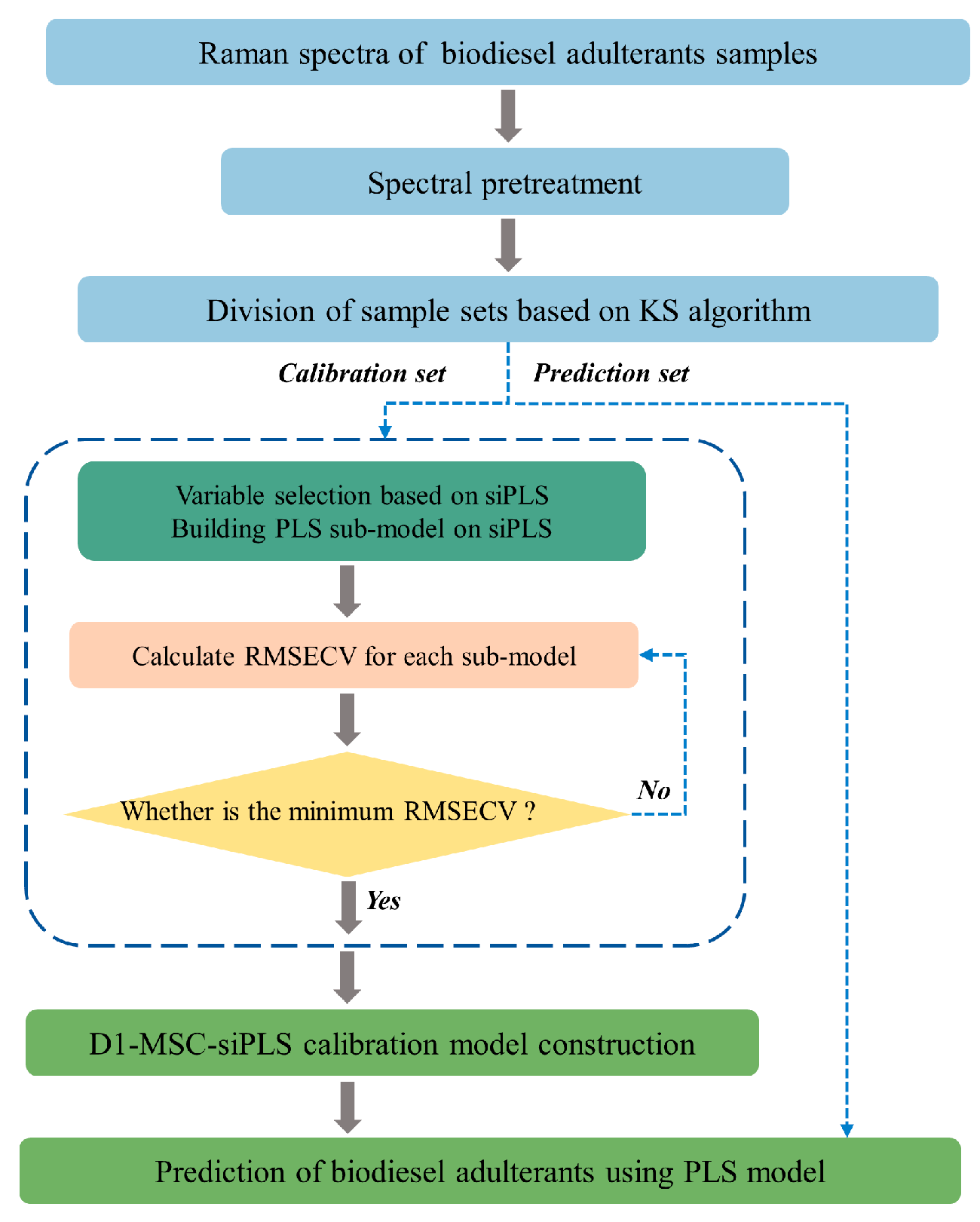
Raman spectra information were collected using a Qepro6500 laser Raman spectrometer (Ocean Optics, Delray Beach, FL, USA) equipped with a 785 nm semiconductor laser. The spectral acquisition range was 0–2000 cm−1, and the laser power was 300 mW. Prior to each sample acquisition, background spectra were acquired using a clean, empty cuvette. The resolution was 4 cm−1 and the ambient was 20 °C during the acquisition. Measurements were repeated 5 times for each sample, and the mean spectra were taken to build the model.

2.3. siPLS Method

Both the synergy interval partial least squares (siPLS) [43] and the backward interval partial least squares (biPLS) [44] are based on the interval partial least squares (iPLS) approach [45]. iPLS divides the entire spectral region into k equidistant intervals and constructs PLS models on each interval. The sub-intervals in which the local model with the minimum root-mean-square error is located are the characteristic waveband obtained using cross-validation (RMSECV). The biPLS and siPLS approach perform different operations on the spectral data based on the equal division of the full spectrum into k intervals using the iPLS method. Among others, the biPLS divides the spectrum into k equidistant intervals, removes the interval with the lowest correlation among the k intervals, and performs PLS calibration model on the remaining (k-1) joint intervals. This process is repeated iteratively until only one interval remains. The RMSECV value of the PLS model for each subinterval was used as an evaluation metric, with the minimum value corresponding to the best combination interval. In contrast, the siPLS randomly selects sets of j (2 ≤ j ≤ k) sub-intervals from the k intervals and builds PLS models. The combination of j intervals corresponding to the minimum RMSECV value represents the optimal spectral wavebands. The advantage of siPLS over iPLS and biPLS is that it improves the predictive power of effective components of the model by combining several partial models with higher precisions in multiple equidistant sub-intervals to find the most relevant regions of information.

2.4. Construction and Evaluation of Calibration Models

Spectral data preprocessing is an important step to address the interference factors such as noise, over-lapping peaks, and baselines affecting the spectra in establishing accurate quantitative analysis models. Firstly, spectral preprocessing was performed to eliminate noise from the raw spectra where the modelled performance was disturbing. Simultaneously, the Kennard–Stone method (sample-set division based on calculation of distances in the x-vector direction) was employed to separate the preprocessed spectral data into a calibration set (70%) and a prediction set (30%) (Table 1). Additionally, variable selection methods helped to fully utilize relevant variables that contributed to predictive performance. Therefore, characteristic intervals were selected using siPLS in the spectral range of 0–2000 cm−1, and combinations of 2–4 intervals were used as input variables to construct all possible PLS quantitative analysis models. Finally, the lowest RMSECV value obtained using the PLS model was selected as the feature interval. The optimal number of latent variables (LVs) was determined by the results of the best cross-validation (CV). The determination of the accuracy of the prediction results was dependent on the agreement between the PLS model predictions and the reference values. Multiple metrics were used to evaluate the predictive performance of the model, including mean relative error of prediction (MREP), determination coefficient of prediction (R2P), root-mean-squared error of prediction (RMSEP), and residual predictive deviation (RPD). Leave-one-out cross-validation (LOO-CV) was employed to assess the stability of the models. All calculations were implemented using MATLAB (2016b). The modeling process is illustrated in Figure 1.

3. Results and Discussion

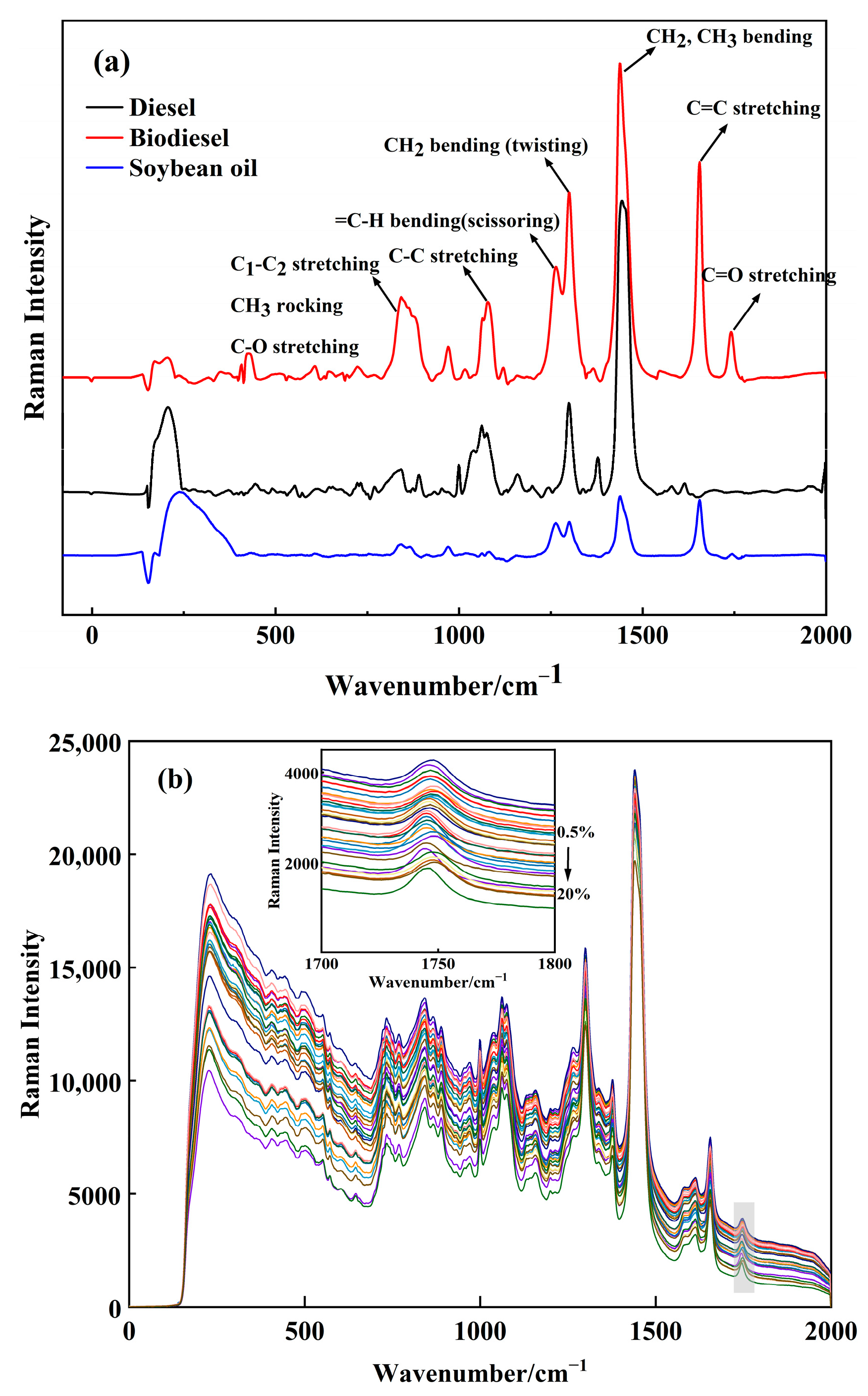
3.1. Raman Spectral of Biodiesel

Raman spectra of pure diesel, pure biodiesel and pure soybean oil that have been baseline-corrected to reduce the linear variation across the in the 0–2000 cm−1 range are shown in Figure 2a. It can be seen from the spectrogram that the characteristic peaks of the three oils were as follows: for diesel, the relevant vibrations were attributed to C1–C2 stretching, in-plane CH3 rocking, and C-O stretching (800–900 cm−1), C-C stretching (1050–1150 cm−1), =C-H bending (1245–1277 cm−1), and CH2/CH3 bending vibrations (1400–1500 cm−1) [2]. In comparison to diesel, biodiesel exhibited characteristic bands related to CH2 bending (1290–1320 cm−1), C=C stretching (1600–1700 cm−1), and C=O stretching vibrations (1700–1800 cm−1) [30]. As for soybean oil, its characteristic bands were highly similar to those of biodiesel, including C=C bending (968 cm−1), C-H bending (1245–1300 cm−1), C=C stretching (1600–1700 cm−1), and C=O stretching vibrations (1700–1800 cm−1) [46]. This is consistent with the conclusion drawn in the relevant literature. The Raman spectra of different fuels differed in their fingerprint region and range, enabling the compounds present in each sample to be identified. It can be seen from Figure 2b that the Raman spectra showed certain variations as the biodiesel content in the fuel increased: a change of Raman intensity occurred in the spectra of the different samples, but their Raman shifts of these spectral lines remained relatively constant. As can be seen from the gradual increase in the intensity of the characteristic peak of C=O (1700–1800 cm−1) in the samples, it is possible to obtain information about the biodiesel content by analyzing the characteristic region of the band of adulterated diesel.

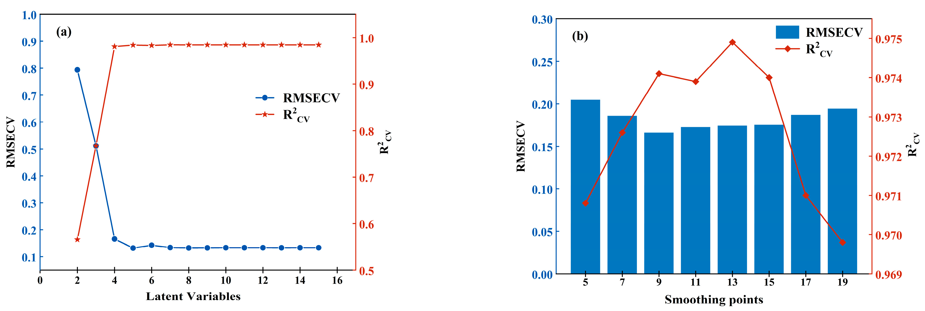
3.2. Optimization of Spectral Preprocessing Methods

During the collection of Raman spectra, various factors such as the collection environment, sample background, and light scattering can introduce significant redundancies into the raw spectra. Therefore, preprocessing of the original Raman spectra is necessary before constructing the PLS calibration model. This study compared different spectral preprocessing methods, including normalization (Nor), standard normal variation (SNV), wavelet transform (WT) [47], first-order derivation (D1st), and multivariate scatter correction (MSC) [30], as well as their different combinations, to investigate their effects on the calibration model of PLS. The D1st preprocessing method effectively removes baseline drift and background noise, which increases peak resolution and improves the signal-to-noise ratio. MSC and SNV have similar purposes and are mainly used to eliminate the influence of physical factors, such as variations in the spectral range and solid particle size, on spectral data. Spectral analysis showed that the preprocessed spectra exhibited richer peaks, clearer waveforms and higher resolution. The model evaluation criteria were R2CV and RMSECV. As shown in Table 2, D1st was the optimal individual preprocessing method (R2CV = 0.9741, RMSECV = 0.1661% (v/v)). Compared to the original spectra (R2CV of 0.9738 and RMSECV of 0.1912% (v/v)), the PLS calibration model achieved significant improvements. The others preprocessing methods, i.e., Nor, SNV, WT, and MSC, did not enhance the R2CV and RMSECV of the model; instead, they led to a decrease in performance. However, a slightly better prediction performance was observed for the prediction dataset after applying the Nor and MSC methods, with R2p values increasing from 0.9868 to 0.9894 and 0.9896, respectively.
The three preprocessing methods, D1st, MMS and MSC, which have different enhancements to the model, were combined in various forms. It was finally determined that the spectral data obtained after D1-MSC preprocessing would be used as input variables for establishing the calibration model. Combined with the optimal LVs (5), the D1-MSC-PLS model achieved an R2CV of 0.9812 and an RMSECV of 0.1558% (v/v). When this model was used for prediction, the R2P was 0.9932, the RMSEP was 0.1413% (v/v), and the MREP was 7.10%. These performance indicators showed slight improvements compared to the original spectra (R2P of 0.9868, RMSEP of 0.1654% (v/v), and MREP of 9.51%) and the D1-PLS (R2P of 0.9842, RMSEP of 0.1931% (v/v), and MREP of 11.07%) models, confirming D1-MSC as the effective spectral preprocessing method for constructing the PLS model.
The stability within the model can be increased by optimizing the smoothing points in D1st using LOO-CV. The number of smoothing points is crucial for the D1st method. If the quantity is too small, the denoising effect of the spectrum will be poor, and instead, valuable information may be eliminated, leading to signal distortion. The R2CV and RMSECV were used as indicators to assess model predictive performance. Figure 3b shows that RMSECV decreased and then increased as the number of smoothing points was increased. The minimum RMSECV (0.1661% (v/v)) and optimal R2CV (0.9741) were achieved when the number of smoothing points was 9. At that point, the PLS calibration model exhibited good predictive power. Additionally, the optimization of the model’s latent variables (LVs) [43] was conducted. As shown in Figure 3a, the RMSECV initially decreased and then increased with cross-validation. The minimum RMSECV was reached when the LV was 5. Going beyond 5 LVs increased the risk of overfitting. Therefore, setting 5 the LV for the model was deemed reasonable.

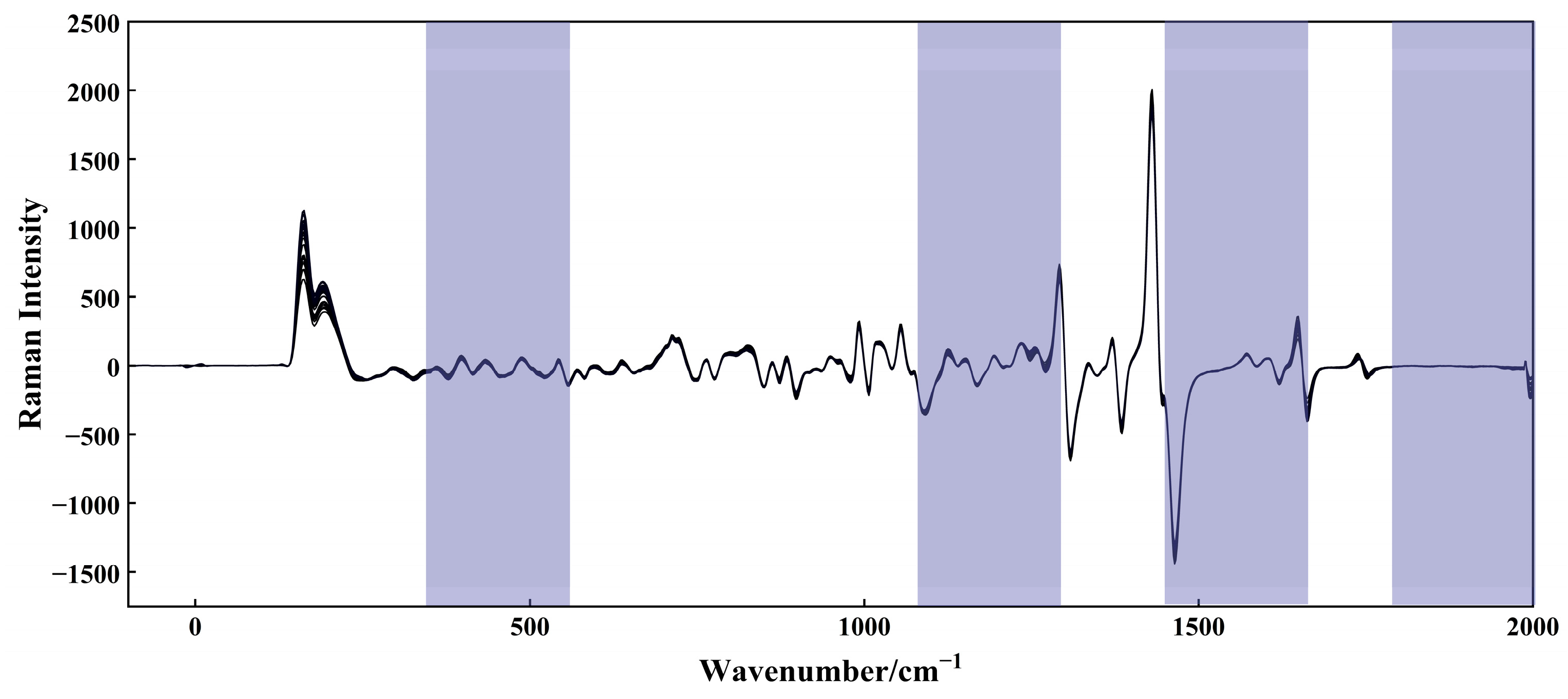
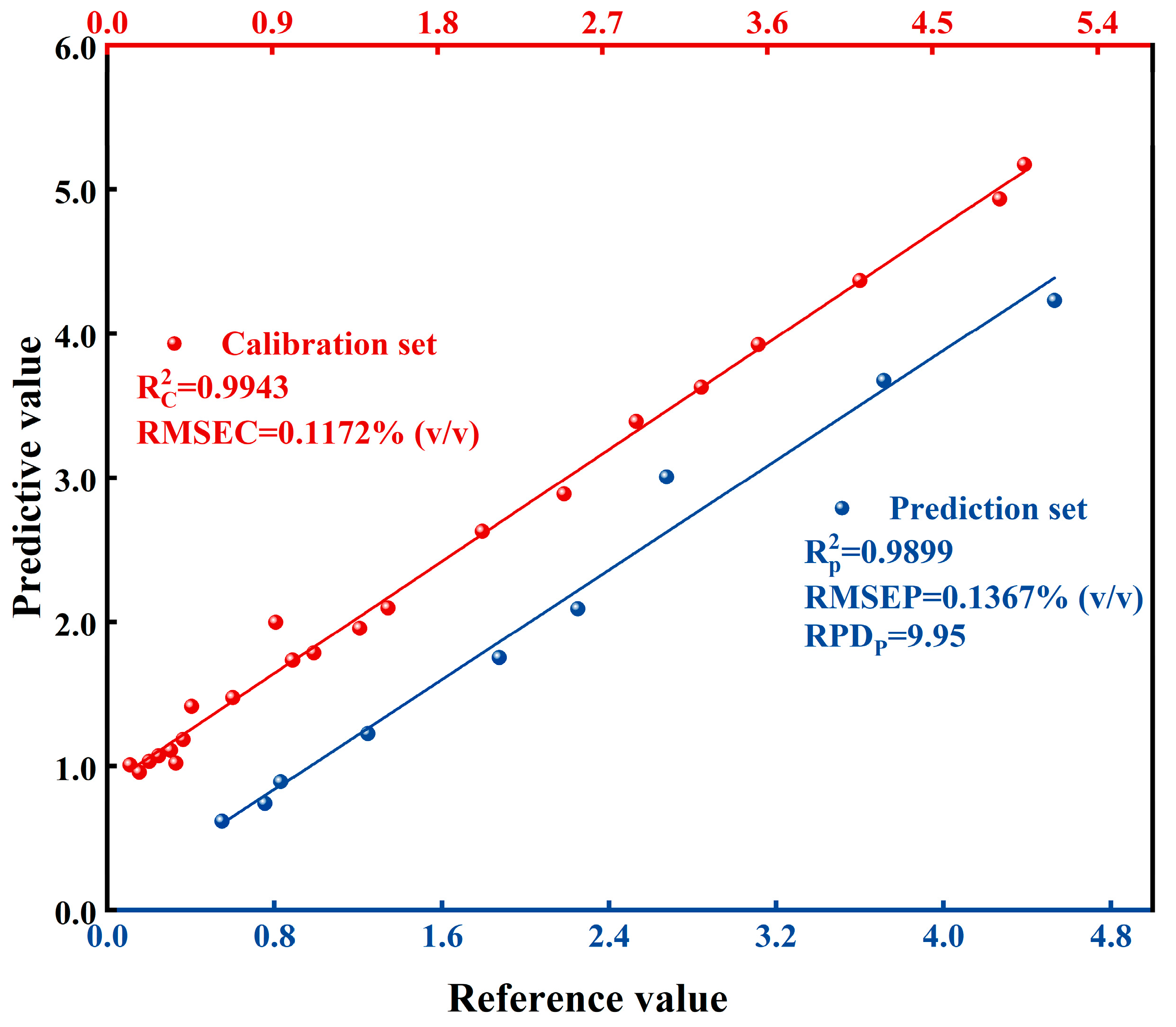
3.3. PLS Calibration Model Based on siPLS Feature Variables Selection

The PLS calibration model based on preprocessed spectral data showed a slight improvement in prediction performance over the original spectra. However, there were still some irrelevant variables in the spectra, as well as multicollinearity among the variables, which not only increased the modelling time and complexity, but also reduced the robustness and accuracy of the model [44]. Therefore, a model is constructed by extracting the relevant variables of the characteristic biodiesel peaks from the whole spectrum as a way to improve the predictive performance of the model [46]. In this study, the method of siPLS was employed to divide the preprocessed spectral matrix (D1-MSC) into 10–20 equal intervals. Since the siPLS algorithm requires selecting combinations of spectral bands and the computational process is complicated, the randomly selected number of sub-interval combinations (j) was typically less than 5. In this experiment, j was set to 2, 3, and 4. Table 3 presents the results of feature subinterval selection by siPLS for different values of k and j. It can be observed that as the quantity of separation intervals decreases and the combination intervals rises, the RMSECV value decreases, indicating the selection of more effective spectral regions. Considering that the RMSEP value is based on the prediction error calculated from the test set data, the high RMSEP value of (siPLS (2)) indicates that the model tends to over-fit under this parameter. However, this problem is overcome as the number of combined intervals increases and the stability of the proposed method is improved. When k = 12 and j = 4, the corresponding R2CV was 0.9842, and the minimum RMSECV was achieved at 0.1329% (v/v).
Figure 4 illustrates the feature variable intervals selected by siPLS, which closely corresponded to the characteristic peaks of C=C stretching and C-H bending in the original spectra. This confirms the feasibility of the siPLS-feature variable selection method. The calculation error expresses the mathematical significance of the model, while the screening of characteristic peaks better corresponds to the physicochemical significance of the study. The optimization of LVs was carried out simultaneously with siPLS variable selection. When LVs were set to 5, the RMSECV of the optimal combination model reached a stable state. The calibration model was then established using the optimal combination (k = 12, j = 4) and the best LVs. The ability of the model to capture variations in measurement data was evaluated using R2, which represents the ability of the independent variables to explain the induced variables. A higher R2 value indicates better fitting performance. The RMSE, which represents the predictive accuracy of the model, is the primary indicator for evaluating the performance of regression models. A lower RMSE value is desirable. RPD is a measure of the predictive power of the model, with higher RPD values indicating better regression performance. Models with RPD values greater than 6 are considered to have good regression performance. The variable selection methods in Table 3 (siPLS (4)) all have better performance on RMSECV compared to PLS (0.9812) after full spectral preprocessing, indicating the necessity of using variable selection as a preprocessing step in spectral detection, and the D1st-MSC-siPLS model showed a significant improvement in predictive performance. The R2CV and R2P values were both above 0.98, and the RMSEP decreased from 0.1413% (v/v) to 0.1367% (v/v). The MREP decreased from 7.10% to 6.31%, while the RPDP was 9.95, indicating the successful modeling of the model.

3.4. Comparison of Different PLS Calibration Models

The performance of the model varied with different preprocessing methods and variable selection methods. Two additional variable selection methods, iPLS and biPLS, were compared to siPLS. To further validate the ability of the D1-MSC-siPLS model to quantify biodiesel, as shown in Table 4, the feature wave numbers were reduced to 87, 261, and 378, selected by the iPLS biPLS and siPLS algorithms, respectively. They were used as input variables to the PLS model to build a quantitative biodiesel model. The siPLS picks out variables that are more included in the location of feature peaks, reflecting the superiority of the algorithms. The cross-validated R2CV of the three feature variable extraction methods was similar, ranging from 0.9738 to 0.9842. However, the RMSECV values of iPLS and biPLS, after variable extraction, decreased from 0.1912% (v/v) to 0.1692% (v/v) and 0.1811% (v/v), respectively, which was not superior to the RMSECV value of siPLS (0.1329% (v/v)). Additionally, both methods had LVs greater than 5, indicating a risk of overfitting. The RMSEP values also did not improve compared to D1st-MSC-siPLS. Among the models, D1st-MSC-biPLS (RMSEP = 0.1879% (v/v)) and D1st-MSC-iPLS (RMSEP = 0.2263% (v/v)) showed marginally improvements in external validation results, but no improvement was observed in cross-validation results. The optimal preprocessing full-spectrum model, D1st-MSC, had an R2P of 0.9932, which was higher than D1st-MSC-siPLS (R2P = 0.9899). However, when R2 is within a reasonable range, MRE is the primary consideration. Therefore, D1st-MSC-siPLS was determined as the optimal model, as it improved the R2CV of the calibration set from 0.9738 to 0.9842, decreased the RMSECV from 0.1912% (v/v) to 0.1329% (v/v), significantly reduced the number of variables from 1044 to 378, decreased the modeling time, and improved the model’s predictive performance.
Figure 5 clearly shows the correlation between the predicted values from the D1st-MSC-siPLS calibration model and the sample standard reference values for biodiesel. Clearly, they exhibited a strong linear relationship. Additionally, the MREP value, in particular, significantly decreased after variable selection. These results demonstrate that spectral preprocessing and appropriate variable selection strategies can significantly enhance the quantity performance of the model. Machine learning methods could be faster and more effective for quantitative analyses of biofuels in adulterated diesel/biodiesel blends.
There are many different approaches in the literature to study the partial or total replacement of biodiesel with different vegetable oils, proving that this issue is very important and should be approached from different perspectives. In the literature, in the batch determination of the identity of biodiesel–diesel blends (concentration and feedstock) by using UFGC, GC has been successfully applied [48]. Liu et al. [2] found that the prediction of biodiesel concentration in blended fuels combined partial least squares (PLS) calibration with the C-H eigenzones of Raman spectroscopy. The quantitative and qualitative analyses of biodiesel using NMR spectroscopic methods were carried out by Doudin [24]. Although there have been many studies that have made significant contributions to the field, there is still a need to develop a rapid detection method to address the quantification of biodiesel in adulterated fuels. Our work is a pioneering study that demonstrates the feasibility of Raman spectroscopy as a quantitative detection technique for biodiesel containing adulterants. In addition, Raman spectroscopy has the potential to be an alternative technique for use by government agencies or quality control laboratories due to its unique capabilities.

4. Conclusions

In this study, a promising model in the accuracy improvement of the ability to quantitatively analyze soybean oil-adulterated biodiesel based on Raman spectroscopy and machine learning methods was presented. The D1-MSC-siPLS correction model was constructed after optimizing the input variables using a D1-MSC preprocessing method and the siPLS feature variable selection method. Compared with the iPLS and biPLS variable selection methods, results elucidate that the D1-MSC-siPLS calibration model is superior in the quantitative analysis of adulterated biodiesel. The cross-validated R2CV of the siPLS calibration set improved from 0.9738 to 0.9842, and the RMSECV decreased from 0.1912% (v/v) to 0.1329% (v/v). Moreover, the number of variables was significantly reduced from 1044 to 378, reducing the modeling time. The model’s predictive performance also improved, with an R2P of 0.9899 and RMSEP decreasing from 0.1654% (v/v) to 0.1367% (v/v), and MREP decreasing from 9.51% to 6.31%. These results demonstrate the feasibility of using Raman spectra combined with the PLS calibration model for the quantitative analysis of biodiesel in adulterated diesel/biodiesel blends.

Author Contributions

Conceptualization, T.Z. and Y.S.; methodology, T.Z. and H.T.; software, Y.S.; validation, C.Y. and M.L.; formal analysis, M.L. and C.Y.; investigation, T.Z. and H.T.; resources, H.L.; data curation, Y.S.; writing—original draft preparation, Y.S.; writing—review and editing, M.L. and T.Z.; visualization, Y.S. and M.L.; supervision, H.L. All authors have read and agreed to the published version of the manuscript.

Funding

This research was funded by the National Natural Science Foundation of China, grant number (22173071, 22303066); Natural Science Basic Research Program of Shaanxi, grant number 2023-JC-QN-0169; and Scientific Research Program Funded by Shaanxi Provincial Education Department, grant number 22JP064.

Institutional Review Board Statement

Not applicable.

Informed Consent Statement

Not applicable.

Data Availability Statement

Not applicable.

Acknowledgments

We are grateful to Yanli Liu of HBIS Institute of Materials Technology for her contribution to this manuscript.

Conflicts of Interest

The authors declare no conflict of interest.

References

  1. Bukkarapu, K.R.; Krishnasamy, A. Support vector regression approach to optimize the biodiesel composition for improved engine performance and lower exhaust emissions. Fuel 2023, 348, 128604. [Google Scholar] [CrossRef]
  2. Liu, Z.; Luo, N.; Shi, J. Raman spectroscopy for the discrimination and quantification of fuel blends. J. Raman. Spectrosc. 2019, 50, 1008–1014. [Google Scholar] [CrossRef]
  3. Barreiros, T.; Young, A.; Cavalcante, R.; Queiroz, E. Impact of biodiesel production on a soybean biorefinery. Renew. Energ. 2020, 159, 1066–1083. [Google Scholar] [CrossRef]
  4. Galhardo, C.E.C.; de Carvalho Rocha, W.F. Exploratory analysis of biodiesel/diesel blends by Kohonen neural networks and infrared spectroscopy. Anal. Methods 2015, 7, 3512–3520. [Google Scholar] [CrossRef]
  5. Carlucci, C. An overview on the production of biodiesel enabled by continuous flow methodologies. Catalysts 2022, 12, 717. [Google Scholar] [CrossRef]
  6. Encinar, J.M.; González, J.F.; Martínez, G.; Nogio-Delgado, S. Use of NaNO3/SiAl as heterogeneous catalyst for fatty acid methyl Ester production from rapeseed oil. Catalysts 2021, 11, 1405. [Google Scholar] [CrossRef]
  7. Nisar, S.; Hanif, M.A.; Rashid, U.; Hanif, A.; Akhtar, M.N.; Ngamcharussrivichai, C. Trends in widely used catalysts for fatty acid methyl esters (Fame) production: A review. Catalysts 2021, 11, 1085. [Google Scholar] [CrossRef]
  8. Máquina, A.D.V.; Sitoe, B.V.; Buiatte, J.E.; Santos, D.Q.; Neto, W.B. Quantification and classification of cotton biodiesel content in diesel blends, using mid-infrared spectroscopy and chemometric methods. Fuel 2019, 237, 373–379. [Google Scholar] [CrossRef]
  9. Yusuff, A.S.; Gbadamosi, A.O.; Popoola, L.T. Biodiesel production from transesterified waste cooking oil by zinc-modified anthill catalyst: Parametric optimization and biodiesel properties improvement. J. Environ. Chem. Eng. 2021, 9, 104955. [Google Scholar] [CrossRef]
  10. Mazivila, S.J. Trends of non-destructive analytical methods for identification of biodiesel feedstock in diesel-biodiesel blend according to European Commission Directive 2012/0288/EC and detecting diesel-biodiesel blend adulteration: A brief review. Talanta 2018, 180, 239–247. [Google Scholar] [CrossRef]
  11. Lou, D.M.; Qi, B.Y.; Zhang, Y.H.; Fang, L. Study on the emission characteristics of urban buses at different emission standards fueled with biodiesel blends. ACS. Omega 2022, 7, 7213–7222. [Google Scholar] [CrossRef]
  12. Hosseini, S.A. Nanocatalysts for biodiesel production. Arab. J. Chem. 2022, 15, 104152. [Google Scholar] [CrossRef]
  13. Cunha, D.A.; Montes, L.F.; Castro, E.V.R. NMR in the time domain: A new methodology to detect adulteration of diesel oil with kerosene. Fuel 2016, 166, 79–85. [Google Scholar] [CrossRef]
  14. Pimentel, M.F.; Ribeiro, G.M.G.S.; da Cruz, R.S.; Luiz, S. Determination of biodiesel content when blended with mineral diesel fuel using infrared spectroscopy and multivariate calibration. Microchem. J. 2006, 82, 201–206. [Google Scholar] [CrossRef]
  15. Câmara, A.B.F.; de Carvalho, L.S.; de Morais, C.L.M. MCR-ALS and PLS coupled to NIR/MIR spectroscopies for quantification and identification of adulterant in biodiesel-diesel blends. Fuel 2017, 210, 497–506. [Google Scholar] [CrossRef]
  16. Zhou, L.; Li, F.S.; Wang, W.C. Determination of total phosphorus in biodiesel by ion chromatography. Microchem. J. 2021, 162, 105875. [Google Scholar] [CrossRef]
  17. de Matos, T.S.; dos Santos, R.C.; de Souza, C.G. Determination of the biodiesel content on biodiesel/diesel blends and their adulteration with vegetable oil by high-performance liquid chromatography. Energy Fuels 2019, 33, 11310–11317. [Google Scholar] [CrossRef]
  18. Hupp, A.M.; Perron, J.; Roques, N.; Crandall, J.; Ramos, S.; Rohrback, B. Analysis of biodiesel-diesel blends using ultrafast gas chromatography (UFGC) and chemometric methods: Extending ASTM D7798 to biodiesel. Fuel 2018, 231, 264–270. [Google Scholar] [CrossRef]
  19. Ling, M.X.; Bian, X.H.; Wang, S.S.; Huang, T. A piecewise mirror extension local mean decomposition method for denoising of near-infrared spectra with uneven noise. Chemometr. Intell. Lab. 2022, 230, 104655. [Google Scholar] [CrossRef]
  20. Mazivila, S.J.; Neto, W.B. Detection of illegal additives in Brazilian S-10/common diesel B7/5 and quantification of Jatropha biodiesel blended with diesel according to EU 2015/1513 by MIR spectroscopy with DD-SIMCA and MCR-ALS under correlation constraint. Fuel 2021, 285, 119159. [Google Scholar] [CrossRef]
  21. Conceição, J.N.; Marangoni, B.S.; Michels, F.S.; Oliveira, I.P. Evaluation of molecular spectroscopy for predicting oxidative degradation of biodiesel and vegetable oil: Correlation analysis between acid value and UV–Vis absorbance and fluorescence. Fuel Process Technol. 2019, 183, 1–7. [Google Scholar] [CrossRef]
  22. Hasnain, S.M.M.; Chatterjee, R.; Sharma, R.P. Spectroscopic performance and emission analysis of Glycine max biodiesel. J. Inst. Eng. (India) Ser. C. 2020, 101, 587–594. [Google Scholar] [CrossRef]
  23. Corgozinho, C.N.C.; Pasa, V.M.D.; Barbeira, P.J.S. Determination of residual oil in diesel oil by spectrofluorimetric and chemometric analysis. Talanta 2008, 76, 479–484. [Google Scholar] [CrossRef] [PubMed]
  24. Doudin, K.I. Quantitative and qualitative analysis of biodiesel by NMR spectroscopic methods. Fuel 2021, 284, 119114. [Google Scholar] [CrossRef]
  25. Shimamoto, G.G.; Bianchessi, L.F.; Tubino, M. Alternative method to quantify biodiesel and vegetable oil in diesel-biodiesel blends through 1H NMR spectroscopy. Talanta 2017, 168, 121–125. [Google Scholar] [CrossRef]
  26. Monteiro, M.R.; Ambrozin, A.R.P.; da Silva Santos, M. Evaluation of biodiesel–diesel blends quality using 1H NMR and chemometrics. Talanta 2009, 78, 660–664. [Google Scholar] [CrossRef]
  27. Dos Santos, V.H.J.M.; Ramos, A.S.; Pires, J.P. Discriminant analysis of biodiesel fuel blends based on combined data from Fourier Transform Infrared Spectroscopy and stable carbon isotope analysis. Chemometr. Intell. Lab. 2017, 161, 70–78. [Google Scholar] [CrossRef]
  28. Han, L.; Sun, Y.; Wang, S.Y.; Su, T.; Cai, W.S.; Shao, X.G. Understanding the water structures by near-infrared and Raman spectroscopy. J. Raman. Spectrosc. 2022, 53, 1686–1693. [Google Scholar] [CrossRef]
  29. Garcia-Rico, E.; Alvarez-Puebla, R.A.; Guerrini, L. Direct surface-enhanced Raman scattering (SERS) spectroscopy of nucleic acids: From fundamental studies to real-life applications. Chem. Soc. Rev. 2018, 47, 4909–4923. [Google Scholar] [CrossRef]
  30. Ohashi, R.; Fujii, A.; Fukui, K.; Koide, T.; Fukami, T. Non-destructive quantitative analysis of pharmaceutical ointment by transmission Raman spectroscopy. Eur. J. Pharm. Sci. 2022, 169, 106095. [Google Scholar] [CrossRef]
  31. Miranda, A.M.; Castilho-Almeida, E.W.; Ferreira, E.H.M.; Moreira, G.F. Line shape analysis of the Raman spectra from pure and mixed biofuels esters compounds. Fuel 2014, 115, 118–125. [Google Scholar] [CrossRef]
  32. Novikova, N.I.; Matthews, H.; Williams, I.; Sewell, M.A.; Nieuwoudt, M.K. Detecting phytoplankton cell viability using NIR Raman spectroscopy and PCA. ACS. Omega 2022, 7, 5962–5971. [Google Scholar] [CrossRef]
  33. Grosso, R.A.; Walther, A.R.; Brunbech, E.; Sorensen, A.; Schebye, B.; Olsen, K.E. Detection of low numbers of bacterial cells in a pharmaceutical drug product using Raman spectroscopy and PLS-DA multivariate analysis. Analyst 2022, 147, 3593–3603. [Google Scholar] [CrossRef] [PubMed]
  34. Aymen, S.; Nawaz, H.; Majeed, M.I.; Rashid, N.; Ehsan, U. Raman spectroscopy for the quantitative analysis of Lornoxicam in solid dosage forms. J. Raman. Spectrosc. 2023, 54, 250–257. [Google Scholar] [CrossRef]
  35. Pezzotti, G. Raman spectroscopy in cell biology and microbiology. J. Raman. Spectrosc. 2021, 52, 2348–2443. [Google Scholar] [CrossRef]
  36. Orlando, A.; Franceschini, F.; Muscas, C.; Pidkova, S.; Bartoli, M.; Rovere, M.; Tagliaferro, A. A comprehensive review on Raman spectroscopy applications. Chemosensors 2021, 9, 262. [Google Scholar] [CrossRef]
  37. Gallo, E.; Cantu, L.; Duschek, F. Remote Raman spectroscopy of explosive precursors. Opt. Eng. 2021, 60, 084108. [Google Scholar] [CrossRef]
  38. Dodo, K.; Fujita, K.; Sodeoka, M. Raman spectroscopy for chemical biology research. J. Am. Chem. Soc. 2022, 144, 19651–19667. [Google Scholar] [CrossRef] [PubMed]
  39. Flecher, P.E.; Welch, W.T.; Albin, S.; Cooper, J.B. Determination of octane numbers and Reid vapor pressure in commercial gasoline using dispersive fiber-optic Raman spectroscopy. Spectrochim. Acta. A 1997, 53, 199–206. [Google Scholar]
  40. Andrade, J.M.; Garrigues, S.; De la Guardia, M.; Gómez-Carracedo, M.; Prada, D. Non-destructive and clean prediction of aviation fuel characteristics through Fourier transform-Raman spectroscopy and multivariate calibration. Anal. Chim. Acta 2003, 482, 115–128. [Google Scholar] [CrossRef]
  41. Mendes, L.S.; Oliveira, F.C.C.; Suarez, P.A.Z.; Rubim, J.C. Determination of ethanol in fuel ethanol and beverages by Fourier transform (FT)-near infrared and FT-Raman spectrometries. Anal. Chim. Acta 2003, 493, 219–231. [Google Scholar] [CrossRef]
  42. Dantas, W.F.C.; Alves, J.C.L.; Poppi, R.J. MCR-ALS with correlation constraint and Raman spectroscopy for identification and quantification of biofuels and adulterants in petroleum diesel. Chemometr. Intell. Lab. 2017, 169, 116–121. [Google Scholar] [CrossRef]
  43. Pereira Rainha, K.; Tristão do Carmo Rocha, J.; Tavares Rodrigues, R.R.; de Oliveira Lovattiet, B.P. Determination of API gravity and total and basic nitrogen content by mid-and near-infrared spectroscopy in crude oil with multivariate regression and variable selection tools. Anal. Lett. 2019, 52, 2914–2930. [Google Scholar] [CrossRef]
  44. Li, W.; Tan, F.; Cui, J.P.; Ma, B. Fast identification of soybean varieties using Raman spectroscopy. Vib. Spectrosc. 2022, 123, 103447. [Google Scholar] [CrossRef]
  45. Geng, J.X.; Yang, C.H.; Luo, Q.W.; Lan, L.J.; Li, Y.G. iPCPA: Interval permutation combination population analysis for spectral wavelength selection. Anal. Chim. Acta 2021, 1171, 338635. [Google Scholar] [CrossRef]
  46. Firdous, S.; Anwar, S.; Waheed, A.; Maraj, M. Optical characterization of pure vegetable oils and their biodiesels using Raman spectroscopy. Laser Physics. 2016, 26, 046001. [Google Scholar] [CrossRef]
  47. Tong, X.; Zhang, Z.M.; Zeng, F.J.; Liang, Y.Z. Recursive wavelet peak detection of analytical signals. Chromatographia 2016, 79, 1247–1255. [Google Scholar] [CrossRef]
  48. Ramos, K.; Riddell, A.; Tsiagras, H. Analysis of biodiesel-diesel blends: Does ultrafast gas chromatography provide for similar separation in a fraction of the time? J. Chromatogr. A 2022, 1667, 462903. [Google Scholar] [CrossRef]
Figure 1. Research flow chart of the work.
Applsci 13 11306 g001
Figure 2. Raman spectra of different samples ((a): pure samples of diesel, biodiesel, and soybean; (b): samples with different biodiesel contents).
Applsci 13 11306 g002
Figure 3. Predictive performance of PLS models with different parameters ((a): the effect of latent variables; (b): the effect of different smoothing points of D1st).
Applsci 13 11306 g003
Figure 4. Feature variables selected using siPLS.
Applsci 13 11306 g004
Figure 5. The prediction performance of the model proposed in this work for biodiesel adulterants.
Applsci 13 11306 g005
Table 1. Volume percentages of each component in fuel samples.
No.Biodiesel/% (v/v)Soybean Oil/% (v/v)Diesel/% (v/v)No.Biodiesel/% (v/v)Soybean Oil/% (v/v)Diesel/% (v/v)
120.00 0.00 80.00 174.50 13.06 82.44
219.46 5.54 75.00 184.04 13.02 82.94
3 *18.12 6.12 75.76 193.68 12.98 83.34
416.42 6.18 77.40 20 *3.32 12.88 83.80
5 *14.86 5.14 79.00 21 *3.02 16.76 80.22
614.20 5.82 79.98 222.74 16.56 80.70
712.96 2.04 85.00 23 *2.20 16.90 80.90
811.54 4.46 84.00 241.84 16.22 81.94
9 *10.70 4.70 84.60 251.66 16.66 81.68
109.96 10.42 79.62 261.50 18.50 80.00
11 *9.00 11.50 79.50 271.38 16.36 82.26
128.18 8.02 83.80 281.12 17.10 81.78
13 *7.50 12.80 79.70 290.92 17.76 81.32
146.12 12.38 81.50 300.70 19.30 80.00
155.50 12.74 81.76 310.50 19.50 80.00
16 *4.98 12.94 82.08
Note: The samples marked with an asterisk (*) represent 9 independent test sets, while the remaining 22 samples serve as the calibration set. The total volume of each sample is 25 mL.
Table 2. Comparison of predictive performance of synergy interval partial least squares (PLS) calibration models based on different spectral preprocessing methods.
Preprocessing MethodsLVsLOO-CVPrediction Set
R2CVRMSECV% (v/v)R2pRMSEP% (v/v)MREP/%
Raw 70.97380.19120.98680.16549.51
Nor80.96600.21750.98940.15908.93
MSC80.96560.22540.98960.23809.96
SNV80.96850.21720.98420.254910.76
WT (k = 4, db3)100.96680.21500.98040.205514.71
D2st-1760.96870.19680.98600.181510.00
D1st-960.97410.16610.98420.193111.07
Nor-D1st60.96960.19520.99230.15377.85
D1st-MSC50.98120.15580.99320.14137.10
Note: k means decomposition layers, db3 means wavelet function.
Table 3. Cross-validation results of PLS calibration models with different separation intervals and different combinations of interval numbers.
Variable
Extract
Interval NumberVariable
Number
LOO-CVPrediction Set
R2CVRMSECV% (v/v)R2PRMSEP% (v/v)MREP/%RPDP
siPLS (2)121890.97710.17100.97710.238611.656.61
151740.93780.35060.88370.357926.542.93
181610.92490.35590.90530.334620.093.25
201490.93370.34400.82070.368229.382.36
siPLS (3)122840.98390.13550.96820.15078.515.61
152610.98390.13550.97420.181714.446.23
182410.98090.15680.96190.198613.295.12
202240.98140.15860.98880.17157.999.45
siPLS (4)123790.98420.13290.98990.13676.319.95
153480.98390.14090.97650.265213.476.52
183210.98110.15630.96360.291612.765.24
202990.98060.16220.98910.17808.349.58
Table 4. Comparison of predictive performances of PLS calibration models.
Calibration
Models
LVsVariable
Number
LOO-CVPrediction Set
R2cvRMSECV% (v/v)R2PRMSEP% (v/v)MREP/%RPDP
PLS710440.97380.19120.98680.16549.518.70
D1st610440.97410.16610.98420.193111.077.96
D1st -MSC510440.98120.15580.99320.14137.1012.13
D1st-MSC-siPLS53780.98420.13290.98990.13676.319.95
D1st-MSC-iPLS6870.97980.16920.98530.226313.418.25
D1st-MSC-biPLS72610.97800.18110.98370.18799.597.83
Disclaimer/Publisher’s Note: The statements, opinions and data contained in all publications are solely those of the individual author(s) and contributor(s) and not of MDPI and/or the editor(s). MDPI and/or the editor(s) disclaim responsibility for any injury to people or property resulting from any ideas, methods, instructions or products referred to in the content.

