Article

Cold and Wet Mantle Transition Zone Beneath the Mediterranean Sea Revealed by the Electrical Image

College of Geo-Exploration Science and Technology, Jilin University, Changchun 130026, China
*
Author to whom correspondence should be addressed.
Appl. Sci. 2023, 13(2), 689; https://doi.org/10.3390/app13020689
Submission received: 5 December 2022 / Revised: 29 December 2022 / Accepted: 1 January 2023 / Published: 4 January 2023

Abstract

:

Featured Application

Electrical structure of the mantle transition zone beneath the Mediterranean Sea is derived from long-term geomagnetic data through the application of electromagnetic induction. Using the conductivity model established according to laboratory measurements, the property of the mantle transition zone is analyzed.

Abstract

A three-dimensional electrical conductivity model of the mantle beneath North Africa and Southern Europe is obtained by geomagnetic depth sounding. C-responses are estimated from geomagnetic data observed at observatories in and around the region and converted to the electrical structure of the mantle transition zone. The limited-memory quasi-Newton method is chosen to minimize the nonlinear objective function of inversion, while the forward modeling relies on a staggered-grid finite difference method in the spherical coordinate system. The data misfit term of the inversion function is measured using the L1-norm in order to suppress the response instability caused by the significant noise contained in the observed data. In order to adequately correct the ocean effect in observatories near the coast, a fixed shell comprised of ocean and land is incorporated in inversion. A banded zone with reduced conductivity is present in the three-dimensional model, primarily seen in the lower mantle transition zone and lower mantle beneath the Mediterranean Sea. Combining laboratory-measured conductivity models, we propose that subducted slabs causing reduced temperature and a water reservoir in the mantle transition zone should be responsible for the observed electrical model.

1. Introduction

Mantle plumes and subducting slabs can transport material upwards and downwards in the earth, and they play essential roles in Earth’s convection and evolution [1,2]. Although the plumes and slabs can be disclosed by geophysical observations [3,4,5,6], their small scale compared with the mantle has hindered their direct observation. Plumes and slabs will react with the mantle transition zone (MTZ) when passing through it, particularly with the 410 km and 670 km phase transition interfaces. The 670 km discontinuity hinders the subduction of slabs, resulting in a stagnant slab along the interface, such as the stagnant Pacific Slab beneath Northeast Asia [6,7,8,9], and it blocks the upwelling mantle plumes, resulting in the accumulation of plume materials and forming a broad head thousands of kilometers in diameter, such as the plume models established by Maguire [4,5]. These reactions make the detection of MTZ significant in the search for the secrets of Earth.
Geophysical methods, particularly seismic imaging, have been widely used to detect the structure of Earth [10,11,12]. Seismic imaging has shown strong evidence for mantle plumes and subducting slabs [6,7,11]. The observed heterogeneities of Earth based on seismic velocity variations may be caused by the thermochemical fluctuations associated with the underlying processes in the mantle, but a defined description has not yet been given. Obtaining additional information on the structure of Earth is an effective way to solve this challenge.
The electrical conductivity of the mantle is strongly sensitive to variations of temperature, mineral composition, oxidation–deoxidation environment, extent of hydration, and melt state [13,14,15,16], even more obviously than elasticity, which governs seismic velocity. Therefore, measuring the electrical conductivity of the mantle has great potential for mapping the chemical and physical structure of Earth and offers a complementary approach to tomography investigation.
The deep electrical structure of Earth can be probed with geomagnetic depth sounding (GDS) [17,18]. GDS has been used to detect variations in the MTZ beneath Australia [15] and East Asia [19,20], demonstrating its advantages in the research of deep Earth. The first global-scale three-dimensional (3D) image of electrical conductivity variations in Earth’s mantle was derived from long-term geomagnetic data through electromagnetic (EM) induction [3,17,21]. It demonstrates a heterogeneous MTZ and provides evidence for the influence of subducting slabs and mantle plumes [3,17,21]. In particular, beneath North Africa and Southern Europe, a large-scale resistive structure is found in the MTZ, which should be caused by less water, lower temperature, or changed mineral composition in the region compared with the normal MTZ [22]. However, little attention has been paid to conducting a detailed analysis of the origin of this structure. This could be attributed to the rough model obtained by global-scale inversion, which used a large grid interval of approximately 10° to parameterize Earth’s electrical field and limits the cognition of structures on regional or local scales. Besides the African and European plates that meet in this area, the Calabria (CAL) and Hellenic (HEL) slabs have subducted into the deep mantle, as imaged by seismic tomography [23]. These subducting slabs cause a series of impacts on the mantle, such as reduced temperature and increased water content near the pathway of the slab, which can introduce a significant reduction in electrical conductivity [14,24]. Therefore, it is necessary to undertake further analysis of the electrical structure of the area. In this paper, we will reprocess the geomagnetic data in North Africa and Southern Europe, especially regions in Southern Europe with dense observatories, and perform 3D EM inversion with a finer grid in order to obtain a more precise electrical structure of the mantle by applying the method we presented previously [3]. Combined with the measured electrical conductivity of the primary minerals of Earth under high-temperature and high-pressure (HTHP) conditions, we will further analyze the nature of the structure and seek its formation mechanism.

2. Data and Methods

2.1. Theory of GDS

GDS is a type of EM induction with long-period changing ring currents in the magnetosphere [25]. The period of the geomagnetic field ranges from about several days to more than a hundred days, and GDS can detect the electrical conductivity of the mantle from the depth 200 km to 1600 km. The ring currents in the magnetosphere are concentric with the magnetic equator of Earth, so numerical modeling is conducted in the geomagnetic spherical coordinate system. The C-response of GDS is widely used and can be obtained through the recorded vertical component ( H r ), pointing downwards toward the center of the Earth, and the co-latitudinal ( H θ ) components, pointing toward magnetic north pole, of the magnetic field (H) on Earth’s surface. A single spherical harmonic function P 1 0 is assumed to describe the inducing currents [17,25,26,27], and C-response can be determined by
C ( ω ) = a 0 tan θ 2 H r ( ω ) H θ ( ω )
where a 0 is the average radius of Earth (approximately 6371 km), ω is the angular frequency, and θ represents the geomagnetic colatitude (0°–180°).
Equation (1) shows that C-responses are related to the components of H. If a positive time harmonic e i ω t is considered, H satisfies
× ( ρ × H ) + i ω μ 0 H = 0.
where ρ is the electrical resistivity, reciprocal with electrical conductivity σ ; μ 0 is the vacuum magnetic permeability; and i is the imaginary unit. The staggered-grid finite difference method developed in a spherical coordinate system [28] is applied to solve Equation (2). Besides the conductive Earth, the resistive air is included into the model’s calculation parameters. The outer boundary of the model’s domain is 2 a 0 from the Earth’s surface, and the resistivity of air is set to 1010 Ω·m. Considering the superconductive core of Earth, the core––mantle boundary is chosen to be the inner boundary of the model domain [25]. We specify the tangential components of the magnetic field at the boundaries in order to ensure that Equation (2) can be calculated throughout the whole model domain, while the resulting numerical modeling system can be well-conditioned. The location of the ring currents is 10 a 0 from the Earth’s surface, measured radially, in order to guarantee that the induced secondary magnetic field of the conductive Earth is negligible. Modification of the biconjugate gradient and an iterative method are utilized to seek the solution of Equation (2) [3]. A divergence correction [29] is applied in order to eliminate the accumulation of error in the calculation of · H .

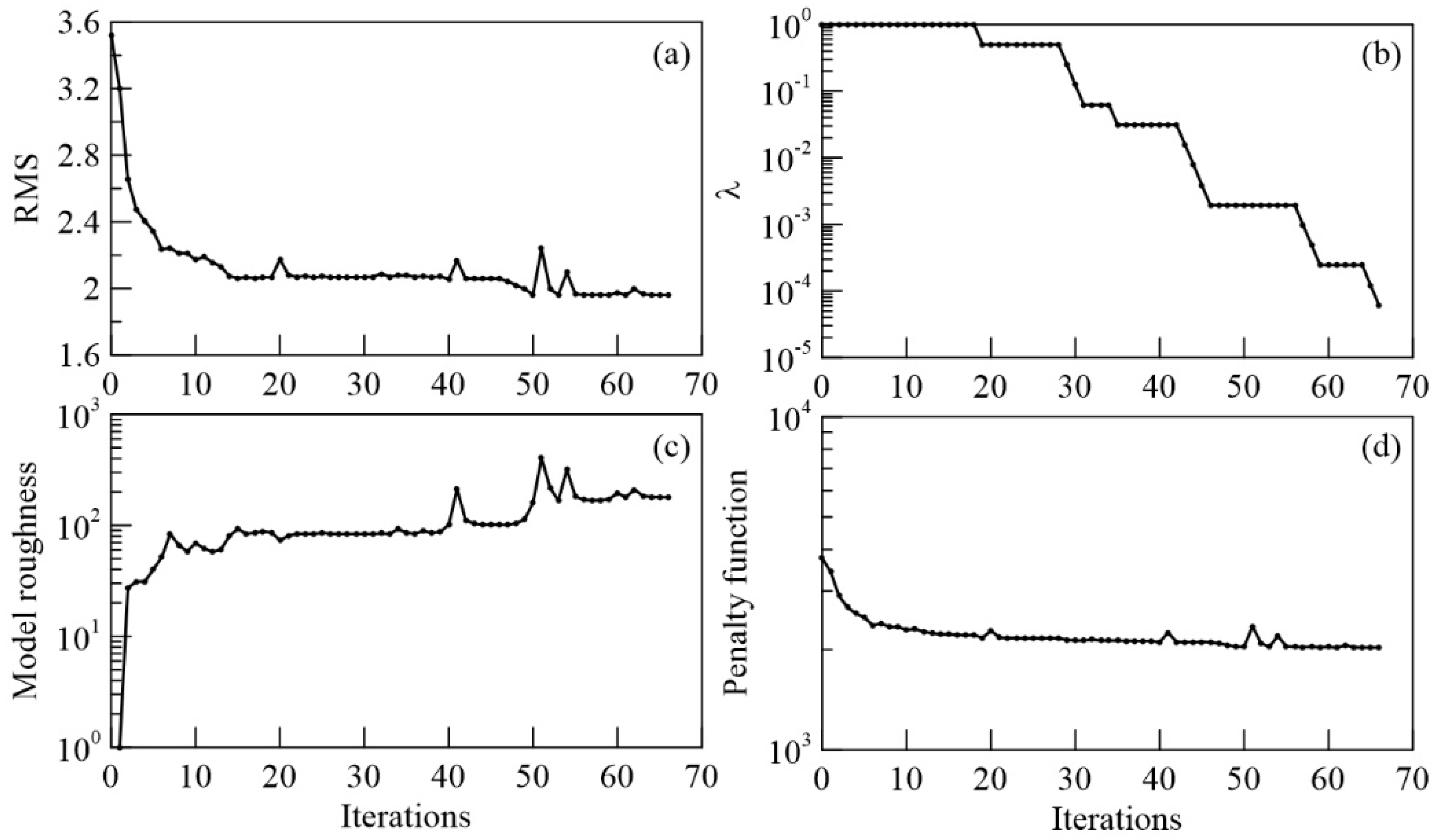
2.2. L-BFGS Inversion

Inversion of GDS can generally be treated as seeking the minimum of
Φ ( m , λ ) m min .
The penalty function Φ ( m , λ ) can be defined by
Φ ( m , λ ) = Φ d ( m ) + λ Φ m ( m ) .
where Φ d ( m ) is the data misfit and Φ m ( m ) is the model roughness; λ is the regularization parameter of the tradeoff Φ d ( m ) and Φ m ( m ) in inversion. m is the model vector and is comprised of the conductivity in each prism in three-dimensional (3D) inversions [6].
An objective function can be expressed as the notation of the Lp-norm measurement, and Equation (4) is expressed as
Φ ( m , λ ) = W d ( ψ ( m ) d ) p p + λ W m ( m m 0 ) p p
where d is the observed data; m 0 is the background model with ψ as the operator of forward modelling; W d is a diagonal matrix comprised of data covariance; and W m is a model smoothing matrix designed to smooth the conductivity with adjacent grids in the X, Y, and Z directions. Smoothness among adjacent cells relates to the value of smoothing coefficients, and the model will be much smoother when coefficients are closer to 1.
Differentiating Equation (5) on both sides with respect to the model parameters and performing a Taylor-series expansion, the equation can be expressed as the following if the higher-order terms of the expansion are neglected,
[ J T W d T R d W d J + λ W m T R m W m ] δ m = J T W d T R d W d [ ψ ( m ) d ] + λ W m T R m W m ( m m 0 ) .
in which,
R j ( x ) = p ( x 2 + ε 2 ) p / 2 1 , j = d o r m
where a small value is given to ε to ensure solving when x = 0 , and p corresponds to the order of Lp-norm inversion.
The nonlinear optimization of Equation (5) is solved using the limited-memory quasi-Newton method (L-BFGS), which has been widely applied in electromagnetic induction detection [30] to seek the solution of penalty functions. The basic iterative progress in L-BFGS is
m k + 1 = m k + α k p k
where
p k = B k 1 Φ k
and
Φ k = ( Φ m 1 , Φ m 2 , , Φ m N ) T | m = m k
Here, k is the number of inversion iterations; α k and p k are the searching step and searching direction, respectively; and B k is the approximation of the Hessian matrix [31]. Employing the approximation matrix can avoid the direct calculation of the Hessian matrix, thus greatly reducing the amount of computer storage and processing time needed.
The calculation of the Jacobian matrix and forward responses are required in the computation of Equation (6). Calculation of the forward responses of a model can be easily carried out. The direct calculation of the Jacobian matrix, however, places high requirements on computing resources, but a more feasible method—adjoint forward technique—is chosen to accomplish the calculation [3,29,32]. Using this technique, the products of the Jacobian matrix and data vector can be separated into a few operations of forward modeling, and thus the computational requirements are greatly reducing.
Considering the strong fluctuation in recorded data at some stations and that a 3D L1-norm inversion [3] in which the data misfit is measured by the L1-norm can suppress the influence of data with substantial noise on the stability of inversion, L1-norm inversion will be conducted in this paper. L1-norm inversion can be realized by setting the value of p to 1.

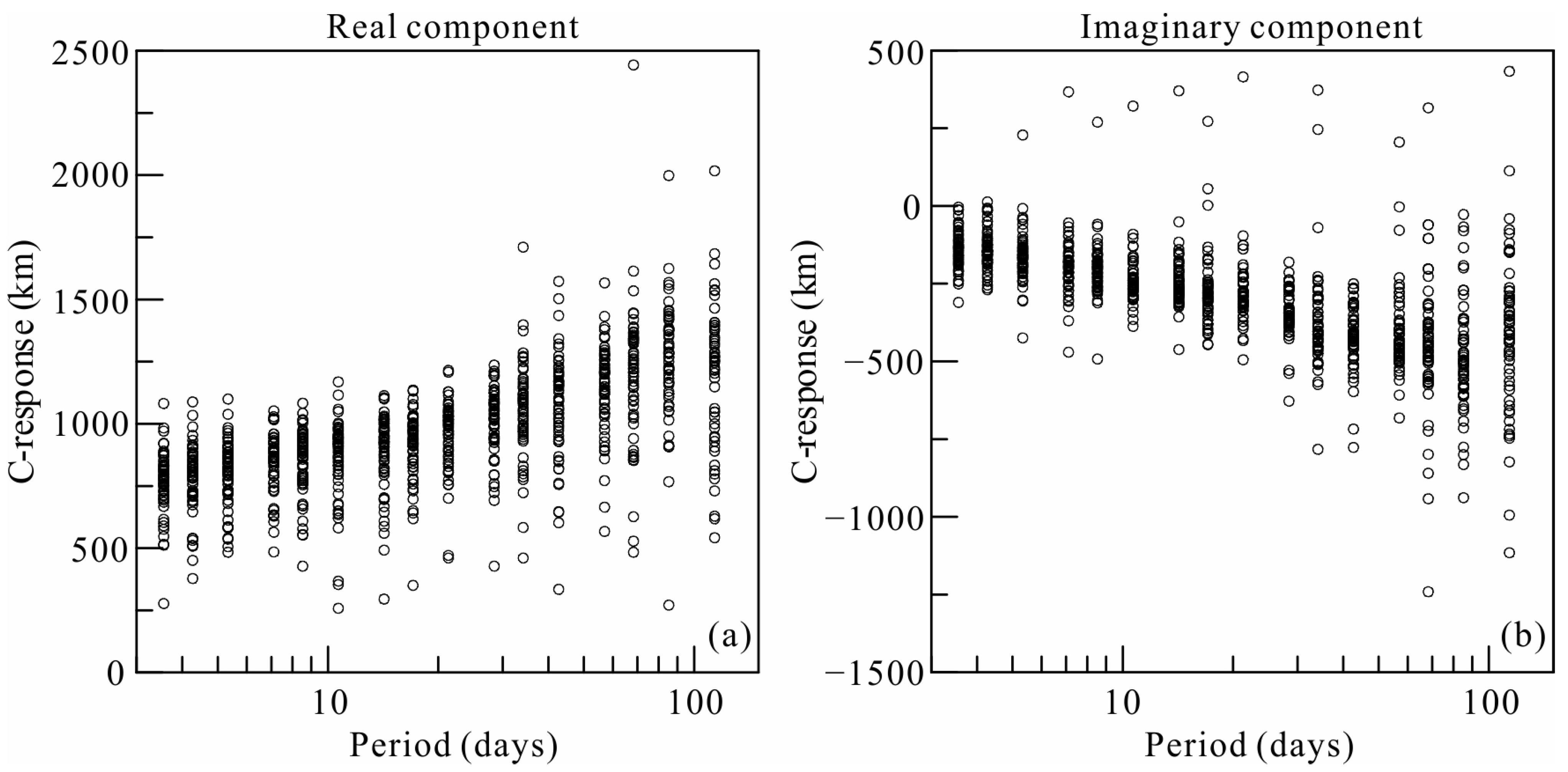
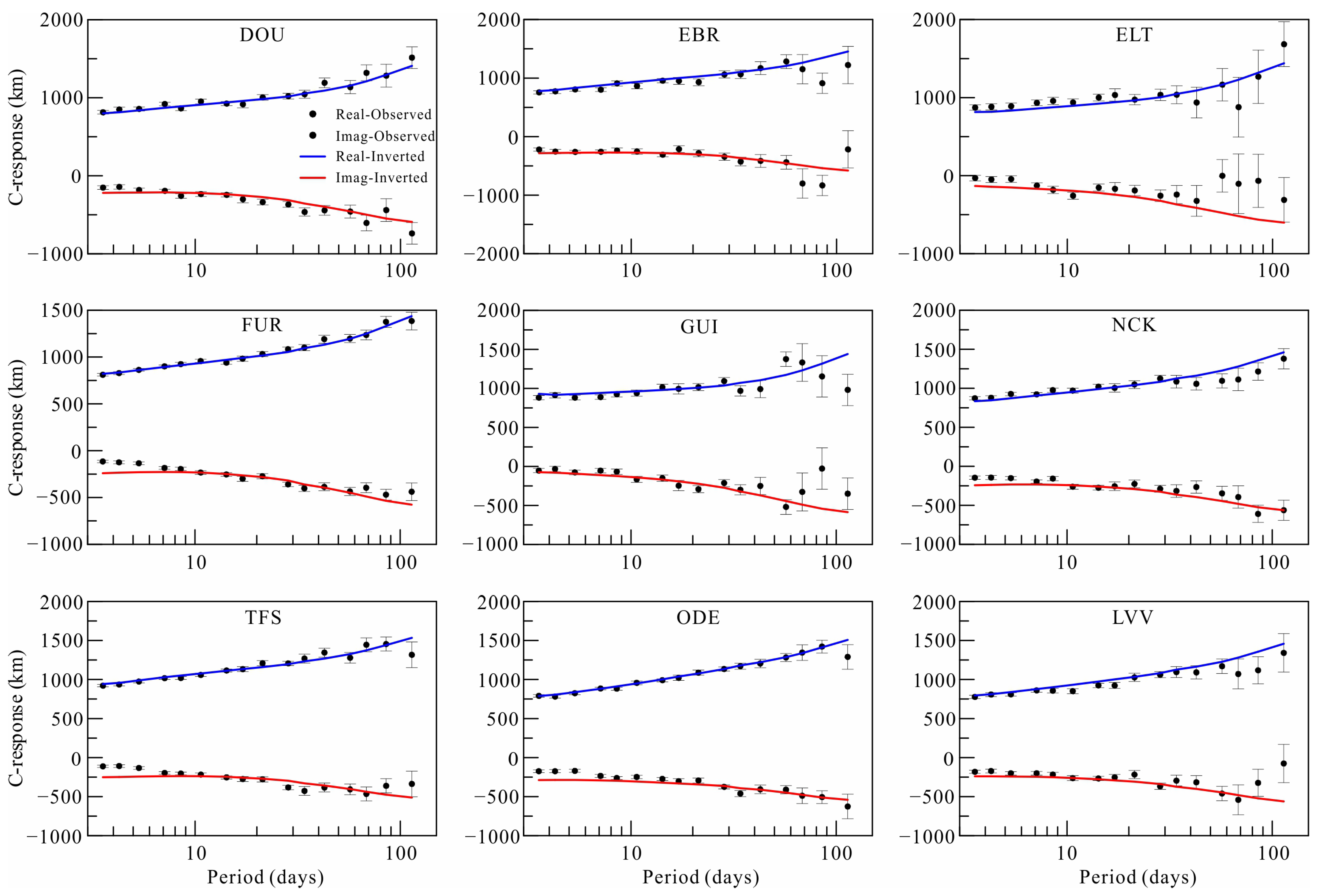
2.3. Data Processing

C-responses can be estimated by the bounded influence of the remote reference processing (BIRRP) method [33]. The method has the capability to eliminate the interference contained in H r and H θ and the correlated noise from both. The remote reference method is used in BIRRP, but the results critically rely on the quality of observed data collected in the remote reference observatory [34,35]. The self-reference method is a wonderful alternative, as its estimation has proven to be closely related to that of the remote reference method for the C-responses used in the present work [21]. Therefore, in this paper, geomagnetic fields are processed using the BIRRP method with self-reference. The hourly mean values time series of three components of the geomagnetic field can be obtained from the World Data Center. Due to the L1-norm inversion used in this paper, we can use as many stations as possible in the following inversion. Therefore, after selection according to the duration and noise, as we presented before [3], we determined 50 geomagnetic observatories in North Africa and Southern Europe for further consideration (Figure 1, Table 1). In order to ensure the data quality, only those recorded after 1950 are used. The length of the selected time series at stations can reach 72 years (1950–2021). C-responses and their errors within 16 periods logarithmically ranging from 3.5 to 113 days at the selected stations are estimated and displayed in Figure 2. The variation in responses at different stations indicates that the electrical structure beneath the area is heterogeneous.

2.4. Influence of Ocean

The C-responses at coastal observatories are significantly influenced by the ocean induction effects caused by the significant electrical conductivity contrasts between conductive oceans and resistive continents, especially for responses with brief durations [21,36,37]. Some of our selected observatories are located near the coastline (Figure 1 and Figure 3), so the responses of the stations impacted by the ocean effect must be corrected. The ratio method can be used for ocean effect correction [36,38], and the specific correction formula is as follows:
C corr = C obs · k ,   and   k = C 1 D / C 1 D + shell
Here, C corr is the corrected response, and C o bs is the observed response at the station; k is the correction coefficient, which can be calculated from the response ( C 1 D ) of the one-dimensional (1D) model and the response ( C 1 D + shell ) of a 1D model with a covering shell comprised of oceans and continents. Obviously, the correction coefficient changes with the 1D model. This makes it difficult to search for a perfect 1D model that is suitable for all stations, because the electrical structure of Earth is undiscovered and in three dimensions. Therefore, in our 3D inversion of GDS, the conductivity of the shell with ocean and land is treated as a surface layer of Earth (Figure 3). A lateral grid of 1° × 1° with a thickness of 12.65 km is considered in order to describe the shell more finely [17] and to ensure sufficiently accurate accounting for OIE [36]. The shell will be incorporated in forward numerical but fixed throughout the inversion [3,15].

3. Inversion Results and Stability

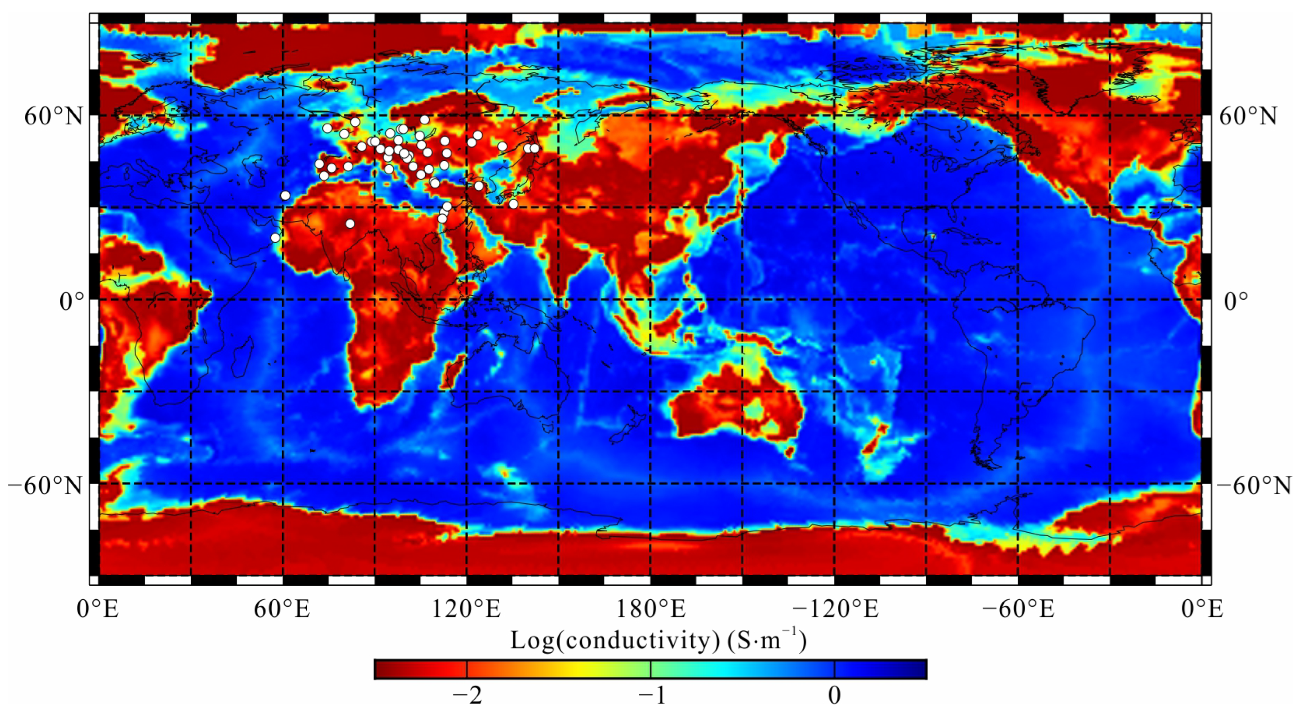
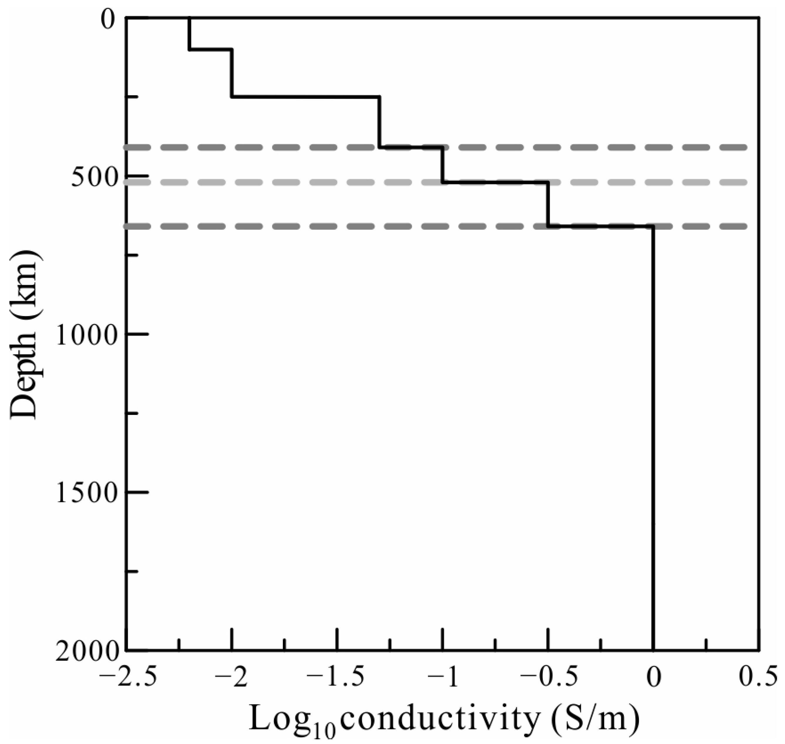
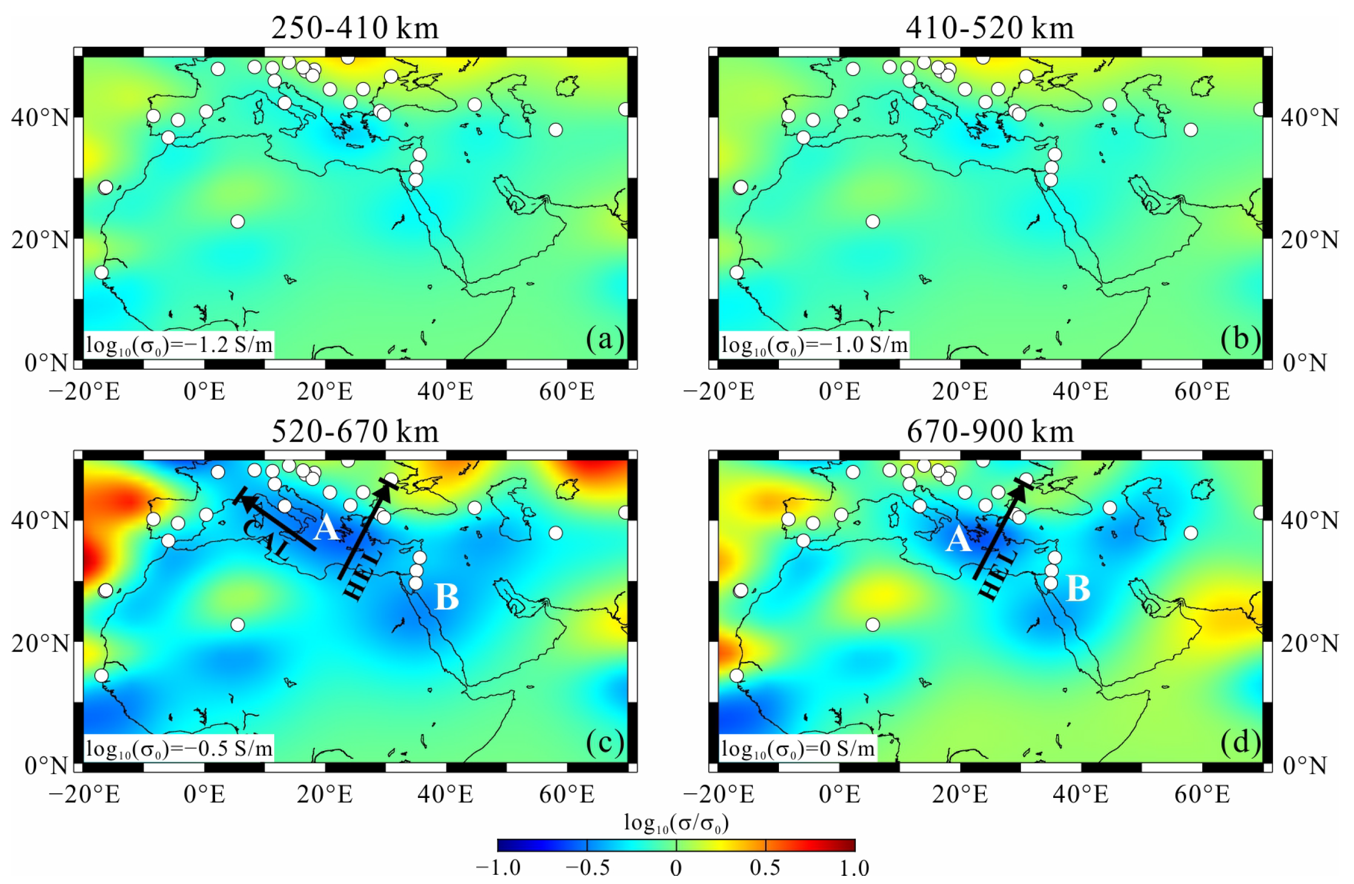
3.1. Electrical Conductivity Model

The C-responses (Figure 2) of the 50 stations in the study area were inverted using a 3D L1-norm GDS method in which the data misfit and model roughness were measured by L1- and L2-norm measurements, respectively. Stations close to the research region were also considered in our inversion in order to reduce the influence of the electrical structures of the surrounding mantle. The data misfit in inversion is normalized using the observed data error derived from the estimated responses, which will be helpful to lessen the weight of these data in inversion. In traditional L2-norm inversion, data with large uncertainties are usually excluded, but in L1-norm inversion, the contributions of unstable data are suppressed by L1-norm measurement and the large data error in normalization. As a result, it is anticipated that we will be able to determine a reliable 3D electrical structure of the mantle beneath North Africa and Southern Europe.
A homogeneous grid is densified as fine as 5° × 5° horizontally in order to discretize the conductive Earth, and the Earth is divided into 12 spherical layers vertically. The conductivity of the initial model for our 3D L1-norm inversion adopts the global average 1D model obtained from the geomagnetic data observed in satellites [39] and depicted in Figure 4. Considering the mineral phase transition interfaces in the mantle, conductivities are allowed to jump at 410 km, 520 km, and 670 km.
The initial regularization parameter of the 3D inversion is set at 1.0. During iterations in which the deviation of the data misfit is below the given threshold value, the regularization parameter is cut in half. The inversion process continues iteratively until the given target data misfit is arrived at or the regularization parameter is rather small. The inversion was conducted with several different regularization parameters in order to better access the stability of the detected anomalies. The results of these inversions demonstrate that the distribution of anomaly is almost similar, except that the sharpness at boundaries is different. After 66 iterations, the inversion terminates when the regularization parameter is smaller than 10−4. The root–mean–square (RMS) error of the data misfit is 1.96 (Figure 5), which is rather larger than the expected value of 1.0. We suggest that this large value is caused by some unreliable responses included in the inversion. This indicates that most of the responses calculated from the inverted model fit the observed data well. The curves in Figure 5 changed slightly when the inversion came to an end, indicating that the inversion result was reliable and that the process was stable. In Figure 6, we show the data fitting curves of the observed data and inverted responses in some stations. The curves show a good consistency for most of the periods of responses, indicating a convincing result of our inversion.
Figure 7 displays the preferred 3D electrical conductivity model near the MTZ (250–900 km) beneath North Africa and Southern Europe. The most attractive feature (anomaly A) is the obviously reduced conductivity area in the lower MTZ and the topmost lower mantle. The electrical structure is similar to that in previous studies [3,17,21] but with a better resolution, and the western portion of the anomaly coincides with the results of Utada et al. [22]. The western portion of the anomaly banding the area extending from the Mediterranean Sea to the Red Sea is named Anomaly A, and the eastern portion spreading from the Red Sea to the Caspian Sea is named Anomaly B. It should be noted that Anomaly A only started from the Eastern Mediterranean in the topmost lower mantle. The strongest variation of anomalies is exhibited beneath Greece in the lower mantle, with conductivity falling to around 1/3 of the global average (Figure 8). The average conductivity of Anomaly A in the lower MTZ appears to be almost twice as resistive as the global average model (Figure 8). In the deep upper mantle and the upper MTZ, only a slight anomaly is present beneath Greece. In addition to the aforementioned anomalies, reduced conductivity zones also appear beneath stations in Africa. Considering the relatively large distance between the stations, these anomalies will not be discussed here.

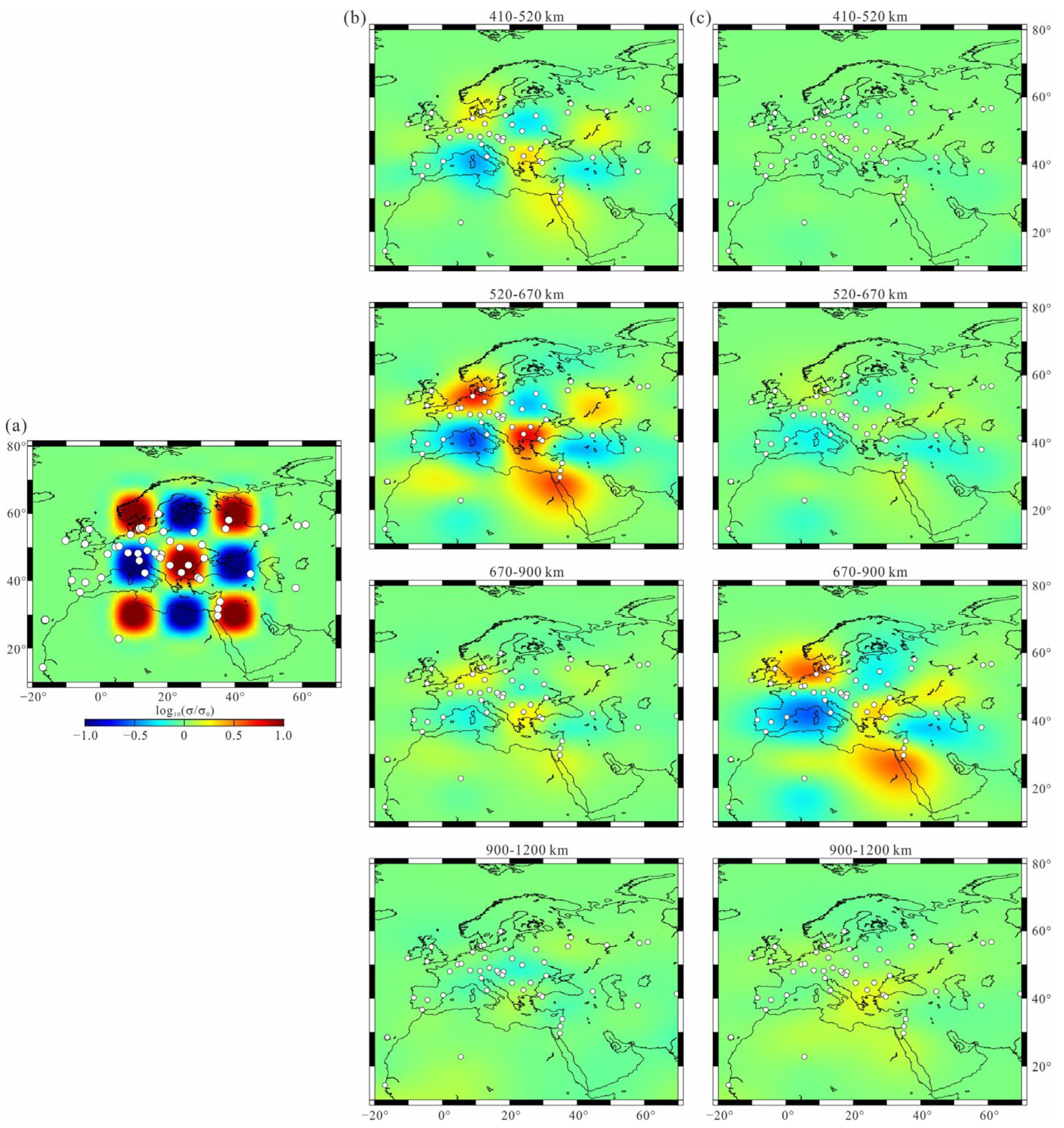
3.2. Robustness of Anomalies

We performed numerical experiments to verify the anomalies. The resolution of the selected stations was tested by a series of GDS inversions with synthetic data generated from checkerboard models. Anomalies in the checkerboard model are on a scale of 10° × 10° (as shown in Figure 8a), and conductivity variations are of one order [ log 10 ( σ / σ 0 ) = 1   and + 1 ] around the magnitude of the background model value. The checkerboard model is set in layers between 520–670 km (Figure 8b) and 670–900 km (Figure 8c), respectively, corresponding to our interested layers. Synthetic data for inversion was generated by adding 5% Gaussian noise to the forward responses at selected stations of the model, and the starting model, initial and changing strategy of regularization parameter, and the other settings of the inversion parameters were the same as those in the preferred inversion. Inversion of the synthetic data (Figure 8) demonstrates that, in regions well covered by stations, the checkerboard structures (10° × 10°) at depths of 520–900 km are resolved relatively well. n particular, the resistive anomaly beneath the Mediterranean Sea is reconstructed both in the shape and amplitude. However, in regions covered by few stations, the conductivity is poorly constrained. The resolution tests demonstrate that our inverted model is in the distinguishable range of GDS with the selected dataset.
In order to determine whether the anomaly is strictly required by the inversion data, we replaced Anomalies A and B at depths of 520 km to 900 km with the conductivity of the background model and then calculated the responses at the selected stations. The curves of the re-forward responses, preferred model responses, and observed data are drawn in Figure 9. It shows that if the anomalies were eliminated, the model–response misfit would become significantly worse at the stations close to the anomaly, such as SFS, PAG, TAM, and QSB. The response shifts a lot from the inverted responses which fit the observed data well, especially for the real components of the C-response, meaning that the conductivity of the reconstructed model is inconsistent with the real situation of the mantle [40]. We, therefore, conclude that the anomaly is a required feature of the data.

4. Discussions

The conductivity of the mantle is influenced by the mineral composition, temperature, and volatiles such as water [14,24]. The conductivity of minerals measured under high-temperature and high-pressure (HTHP) conditions with variable water contents in the laboratory [13] allows us to explore the nature of the anomaly. Compared with conductivity, EM induction is more sensitive to conductance (conductivity × volume) [41], therefore, the inverted average conductivity is more suitable for constraining the range and nature of the true anomalies, while the maximum conductivity can be used to define the center and upper limit of the electrical structure. The average and maximum conductivity of Anomaly A are estimated and drawn in Figure 10.
In the lower mantle, conductivity is determined by temperature and can be estimated by
σ = σ 0 exp ( Δ E + P Δ V k T ) .
Here, σ is the electrical conductivity of the lower mantle, corresponding to the observed bulk electrical conductivity by inversions; σ 0 is the pre-exponential factor and is assuming to be 74 S/m; k is the Boltzmann constant; P is the pressure; and T is the temperature. The values of pressure and temperature at a certain depth of normal mantle can be obtained from the results of Xu et al. [42]. Δ E is the activation energy and Δ V is the activation volume, whose value has been given in Sinmyo et al. [43] from laboratorial measurements. In the topmost lower mantle, the normal temperature is estimated to be approximately 1900 K according to the global average conductivity from Equation (12), and this temperature matches the results presented by Xu et al. [42]. In order to fit the average conductivity of Anomaly A, a temperature at approximately 1400–1600 K, which is 300–500 K lower than the global average (~1900 K), is required (Figure 11a).
In the MTZ, the wadsleyite and ringwoodite have a relatively high capacity of water [1,44,45]. We may estimate the water content and temperature in the lower MTZ according to the electrical conductivity model established by Yoshino et al. [24]:
σ = σ 0 H exp ( H H k T ) + σ 0 P C w exp ( H P 0 α C w 1 / 3 k T ) .
Here, C w is the water content in wadsleyite and ringwoodite; σ 0 is the pre-exponential factor; α and H are constants accounting for geometrical factors and the activation enthalpy. Subscripts H and P denote small polaron and proton conduction, respectively. The normal temperature is approximately 1850 K in the lower MTZ [42]. Figure 11b shows that in the lower MTZ, a 50–150 K-reduced temperature (~1650–1800 K) is required in order to fit the observed conductivity if a global average water content (~0.3 wt.%) was considered, which was estimated according to the global average conductivity obtained by Kelbert et al. [17]. However, the observed conductivity will also be reproduced with the tradeoff between water content and temperature (Figure 11b).
As imaged by tomographic studies, CAL and HEL slabs have been imaged with an improved seismic velocity, which correlates to cold slabs [46], and have penetrated the MTZ [23]. The cold slabs are able to produce the conductivity anomaly we observed. Meanwhile, hydrated minerals in slabs, such as dense hydrous magnesium silicates, will exceed their stable field when the slab is slowly heated by ambient mantle, and the contained water will be released into the MTZ, forming a water reservoir in the MTZ [17,45]. Additionally, tomographic studies also evidence that HEL has passed through the 670 km phase transition interface and sunk to a depth of approximately 1000 km [23]. However, due to the large water capacity of the primary minerals in the lower MTZ (ringwoodite) and lower mantle (bridgmanite), the water in the MTZ and subducting slab will be blocked by the 670 km phase transition interface and stored in MTZ [1,45].
For a rich-water MTZ, the temperature should be much lower than we estimated. If we assume that the subducted slab was adiabatic when passing the 670 km discontinuity, then it shared the same thermal state (approximately 1400–1600 K) in the MTZ and lower mantle, and therefore the water content could reach approximately 0.5 wt% in the lower MTZ. For a more realistic situation, the temperature of the slab is lower in the MTZ than that in the lower mantle, causing a wetter MTZ with a water content higher than 0.5 wt% (Figure 11b). Therefore, we speculate that Anomaly A is caused by the subducting slabs, and that the slab transferred water into the MTZ. The subduction and stagnant location of CAL and HEL are coincident with the morphology of Anomaly A [23], making our deduction more reliable. Compared with the results of Utada et al. [22], a much wetter MTZ is derived in this paper, and we contribute it to the temperature, which is converted from increased seismic wave velocity. Given that water can reduce velocity, a much lower temperature is needed in order to reconstruct the increased velocity if the water is taken into account from the beginning, which leads to more water in the MTZ.
Unfortunately, we are unable to seek the cause of Anomaly B due to a lack of more studies developed in the area. Therefore, the nature of Anomaly B is not discussed in this paper. However, eliminating the influence of cold slabs due to a lack of obviously enhanced seismic wave velocity is imaged [47], and the reduced conductivity caused by temperature or water reduction maybe related to downwelling, which corresponds to the large-scale upwelling beneath the Pacific.

5. Conclusions

In this paper, we present a 3D electrical structure of the mantle with higher resolution than previous studies beneath North Africa and Southern Europe from geomagnetic stations in and around the region. The L1-norm inversion method is used to suppress the influence of data with substantial noise, and model roughness is still measured by an L2-norm as in the traditional inversions used to obtain a smooth model. The BIRRP with self-reference method is used to obtain the C-responses data used in our inversion in periods from 3.5 to 113 days, making GDS sensitive to conductivity near the MTZ.
Checkerboard tests were performed in order to evaluate the resolution of GDS and data sensitivity in the research area. These tests showed that the selected data could invert the electrical structure in the depth range of 520–900 km well. Additional re-forward tests were carried out in order to establish the robustness of the anomaly used in further analysis. These experiments confirmed the reliability and stability of the inverted model.
The inverted model revealed the presence of a banded anomaly with reduced conductivity in the depth range of 520–900 km beneath the Mediterranean Sea. The results of laboratory electrical conductivity of mantle minerals measured under high temperature and high pressure are used to interpret the nature of the anomaly. The anomaly reflects large heterogeneity in water content and temperature in the mantle. Combining the subducted slabs seen by tomography images, we propose that the heterogeneity is induced by the subducted slabs and results in a wet and cold MTZ beneath the Mediterranean Sea.

Author Contributions

Conceptualization, S.L. and Y.L.; methodology, S.L.; software, S.L. and Y.L.; validation, S.L. and Y.L.; investigation, S.L.; resources, Y.L.; data curation, S.L.; writing—original draft preparation, S.L.; writing—review and editing, S.L. and Y.L.; visualization, S.L.; supervision, S.L. and Y.L.; project administration, S.L. and Y.L.; funding acquisition, S.L. and Y.L. All authors have read and agreed to the published version of the manuscript.

Funding

This research was funded by the National Natural Science Foundation of China (grant number 42204076 and 42074120) and the Program for Jilin University Science and Technology Innovative Research Team (2021TD-050).

Institutional Review Board Statement

Not applicable.

Informed Consent Statement

Not applicable.

Data Availability Statement

The data used for inversion can be downloaded from the World Data Centre. The C-responses data that support the findings of this study are available from the authors on reasonable request.

Acknowledgments

The authors thank G.D. Egbert for providing the electromagnetic modeling testbed used to incorporate our inversion method and A.D. Chave for kindly providing the BIRRP software package for the data processing.

Conflicts of Interest

The authors declare no conflict of interest.

References

  1. Bercovici, D.; Karato, S.-I. Whole-Mantle Convection and the Transition-Zone Water Filter. Nature 2003, 425, 39–44. [Google Scholar] [CrossRef] [PubMed]
  2. Koppers, A.A.P.; Becker, T.W.; Jackson, M.G.; Konrad, K.; Müller, R.D.; Romanowicz, B.; Steinberger, B.; Whittaker, J.M. Mantle Plumes and Their Role in Earth Processes. Nat. Rev. Earth Environ. 2021, 2, 382–401. [Google Scholar] [CrossRef]
  3. Li, S.; Weng, A.; Zhang, Y.; Schultz, A.; Li, Y.; Tang, Y.; Zou, Z.; Zhou, Z. Evidence of Bermuda Hot and Wet Upwelling from Novel Three-Dimensional Global Mantle Electrical Conductivity Image. Geochem. Geophys. Geosyst. 2020, 21, e2020GC009016. [Google Scholar] [CrossRef]
  4. Maguire, R.; Ritsema, J.; van Keken, P.E.; Fichtner, A.; Goes, S. P- and S-Wave Delays Caused by Thermal Plumes. Geophys. J. Int. 2016, 206, 1169–1178. [Google Scholar] [CrossRef] [Green Version]
  5. Maguire, R.; Ritsema, J.; Bonnin, M.; van Keken, P.E.; Goes, S. Evaluating the Resolution of Deep Mantle Plumes in Teleseismic Traveltime Tomography. J. Geophys. Res. Solid Earth 2018, 123, 384–400. [Google Scholar] [CrossRef] [Green Version]
  6. Zhao, D. Global Tomographic Images of Mantle Plumes and Subducting Slabs: Insight into Deep Earth Dynamics. Phys. Earth Planet. Inter. 2004, 146, 3–34. [Google Scholar] [CrossRef]
  7. Wang, X.; Chen, Q.F.; Niu, F.; Wei, S.; Ning, J.; Li, J.; Wang, W.; Buchen, J.; Liu, L. Distinct Slab Interfaces Imaged within the Mantle Transition Zone. Nat. Geosci. 2020, 13, 822–827. [Google Scholar] [CrossRef]
  8. Tian, Y.; Zhu, H.; Zhao, D.; Liu, C.; Feng, X.; Liuand, T.; Ma, J. Mantle Transition Zone Structure beneath the Changbai Volcano: Insight into Deep Slab Dehydration and Hot Upwelling near the 410km Discontinuity. J. Geophys. Res. Solid Earth 2016, 121, 5794–5808. [Google Scholar] [CrossRef] [Green Version]
  9. Huang, J.; Zhao, D. High-Resolution Mantle Tomography of China and Surrounding Regions. J. Geophys. Res. Solid Earth 2006, 111, 1–21. [Google Scholar] [CrossRef]
  10. Zahedi, R.; Daneshgar, S.; Ali, M.; Seraji, N.; Asemi, H. Modeling and Interpretation of Geomagnetic Data Related to Geothermal Sources, Northwest of Delijan. Renew. Energy 2022, 196, 444–450. [Google Scholar] [CrossRef]
  11. French, S.W.; Romanowicz, B. Broad Plumes Rooted at the Base of the Earth’s Mantle beneath Major Hotspots. Nature 2015, 525, 95–99. [Google Scholar] [CrossRef]
  12. Zhao, D. Seismic Images under 60 Hotspots: Search for Mantle Plumes. Gondwana Res. 2007, 12, 335–355. [Google Scholar] [CrossRef]
  13. Yoshino, T. Laboratory Electrical Conductivity Measurement of Mantle Minerals. Surv. Geophys. 2010, 31, 163–206. [Google Scholar] [CrossRef] [Green Version]
  14. Karato, S.I. Water Distribution across the Mantle Transition Zone and Its Implications for Global Material Circulation. Earth Planet. Sci. Lett. 2011, 301, 413–423. [Google Scholar] [CrossRef]
  15. Koyama, T.; Khan, A.; Kuvshinov, A. Three-Dimensional Electrical Conductivity Structure beneath Australia from Inversion of Geomagnetic Observatory Data: Evidence for Lateral Variations in Transition-Zone Temperature, Water Content and Melt. Geophys. J. Int. 2014, 196, 1330–1350. [Google Scholar] [CrossRef] [Green Version]
  16. Guo, J.; Lian, X.; Wang, X. Electrical Conductivity Evidence for the Existence of a Mantle Plume beneath Tarim Basin. Appl. Sci. 2021, 11, 893. [Google Scholar] [CrossRef]
  17. Kelbert, A.; Schultz, A.; Egbert, G. Global Electromagnetic Induction Constraints on Transition-Zone Water Content Variations. Nature 2009, 460, 1003–1006. [Google Scholar] [CrossRef]
  18. Chen, C.; Kuvshinov, A.; Kruglyakov, M.; Rigaud, R. Constraining the Crustal and Mantle Conductivity Structures beneath Islands by a Joint Inversion of Multi-Source Magnetic Transfer Functions. J. Geophys. Res. Solid Earth 2023, 128, e2022JB024106. [Google Scholar] [CrossRef]
  19. Zhang, Y.; Weng, A.; Li, S.; Yang, Y.; Tang, Y.; Liu, Y. Electrical Conductivity in the Mantle Transition Zone beneath Eastern China Derived from L1-Norm C-Responses. Geophys. J. Int. 2020, 221, 1110–1124. [Google Scholar] [CrossRef]
  20. Yuan, Y.; Uyeshima, M.; Huang, Q.; Tang, J.; Li, Q.; Teng, Y. Continental-Scale Deep Electrical Resistivity Structure beneath China. Tectonophysics 2020, 790, 228559. [Google Scholar] [CrossRef]
  21. Semenov, A.; Kuvshinov, A. Global 3-D Imaging of Mantle Conductivity Based on Inversion of Observatory C-Responses-II. Data Analysis and Results. Geophys. J. Int. 2012, 191, 965–992. [Google Scholar] [CrossRef] [Green Version]
  22. Utada, H.; Koyama, T.; Obayashi, M.; Fukao, Y. A Joint Interpretation of Electromagnetic and Seismic Tomography Models Suggests the Mantle Transition Zone below Europe Is Dry. Earth Planet. Sci. Lett. 2009, 281, 249–257. [Google Scholar] [CrossRef]
  23. Goes, S.; Agrusta, R.; van Hunen, J.; Garel, F. Subduction-Transition Zone Interaction: A Review. Geosphere 2017, 13, 644–664. [Google Scholar] [CrossRef]
  24. Yoshino, T.; Manthilake, G.; Matsuzaki, T.; Katsura, T. Dry Mantle Transition Zone Inferred from the Conductivity of Wadsleyite and Ringwoodite. Nature 2008, 451, 326–329. [Google Scholar] [CrossRef]
  25. Banks, R.J. Geomagnetic Variations and the Electrical Conductivity of the Upper Mantle. Geophys. J. R. Astron. Soc. 1969, 17, 457–487. [Google Scholar] [CrossRef] [Green Version]
  26. Grayver, A.V.; Munch, F.D.; Kuvshinov, A.V.; Khan, A.; Sabaka, T.J.; Tøffner-Clausen, L. Joint Inversion of Satellite-Detected Tidal and Magnetospheric Signals Constrains Electrical Conductivity and Water Content of the Upper Mantle and Transition Zone. Geophys. Res. Lett. 2017, 44, 6074–6081. [Google Scholar] [CrossRef] [Green Version]
  27. Munch, F.D.; Grayver, A.V.; Kuvshinov, A.; Khan, A. Stochastic Inversion of Geomagnetic Observatory Data Including Rigorous Treatment of the Ocean Induction Effect with Implications for Transition Zone Water Content and Thermal Structure. J. Geophys. Res. Solid Earth 2018, 123, 31–51. [Google Scholar] [CrossRef]
  28. Uyeshima, M.; Schultz, A. Geoelectromagnetic Induction in a Heterogeneous Sphere: A New Three-Dimensional Forward Solver Using a Conservative Staggered-Grid Finite Difference Method. Geophys. J. Int. 2000, 140, 636–650. [Google Scholar] [CrossRef] [Green Version]
  29. Kelbert, A.; Egbert, G.D.; Schultz, A. Non-Linear Conjugate Gradient Inversion for Global EM Induction: Resolution Studies. Geophys. J. Int. 2008, 173, 365–381. [Google Scholar] [CrossRef]
  30. Avdeev, D.; Avdeeva, A. 3D Magnetotelluric Inversion Using a Limited-Memory Quasi-Newton Optimization. Geophysics 2009, 74, F45–F57. [Google Scholar] [CrossRef]
  31. Nocedal, J.; Wright, S.J. Numerical Optimization, 2nd ed.; Mikosch, T.V., Resnick, S.I., Robinson, S.M., Eds.; Springer Science & Business Media, LLC: New York, NY, USA, 2006; Volume 17, ISBN 0196-0202. [Google Scholar]
  32. Egbert, G.D.; Kelbert, A. Computational Recipes for Electromagnetic Inverse Problems. Geophys. J. Int. 2012, 189, 251–267. [Google Scholar] [CrossRef] [Green Version]
  33. Chave, A.D.; Thomson, D.J. Bounded Influence Magnetotelluric Response Function Estimation. Geophys. J. Int. 2004, 157, 988–1006. [Google Scholar] [CrossRef]
  34. Li, G.; Liu, X.; Tang, J.; Deng, J.; Hu, S.; Zhou, C.; Chen, C. Improved Shift—Invariant Sparse Coding for Noise Attenuation of Magnetotelluric Data. Earth Planets Space 2020, 72, 45. [Google Scholar] [CrossRef] [Green Version]
  35. Li, G.; Liu, X.; Tang, J.; Li, J.; Ren, Z.; Chen, C. De-Noising Low-Frequency Magnetotelluric Data Using Mathematical Morphology Fi Ltering and Sparse Representation. J. Appl. Geophys. 2020, 172, 103919. [Google Scholar] [CrossRef]
  36. Chen, C.; Kruglyakov, M.; Kuvshinov, A. A New Method for Accurate and Efficient Modeling of the Local Ocean Induction Effects. Application to Long-Period Responses from Island Geomagnetic Observatories. Geophys. Res. Lett. 2020, 47, e2019GL086351. [Google Scholar] [CrossRef]
  37. Yao, H.; Ren, Z.; Tang, J.; Zhang, K. A Multi-Resolution Finite-Element Approach for Global Electromagnetic Induction Modeling with Application to Southeast China Coastal Geomagnetic Observatory Studies. J. Geophys. Res. Solid Earth 2022, 127, e2022JB024659. [Google Scholar] [CrossRef]
  38. Kuvshinov, A.V. Electromagnetic Induction in the Oceans and the Anomalous Behaviour of Coastal C-Responses for Periods up to 20 Days. Geophys. Res. Lett. 2002, 29, 12–15. [Google Scholar] [CrossRef]
  39. Kuvshinov, A.; Olsen, N. A Global Model of Mantle Conductivity Derived from 5 Years of CHAMP, Ørsted, and SAC-C Magnetic Data. Geophys. Res. Lett. 2006, 33, 1–5. [Google Scholar] [CrossRef]
  40. Schmucker, U. Substitute Conductors for Electromagnetic Response Estimates. Pure Appl. Geophys. 1987, 125, 341–367. [Google Scholar] [CrossRef]
  41. Key, K.; Constable, S.; Liu, L.; Pommier, A. Electrical Image of Passive Mantle Upwelling beneath the Northern East Pacific Rise. Nature 2013, 495, 499–502. [Google Scholar] [CrossRef]
  42. Xu, Y.; Shankland, T.J.; Poe, B.T. Laboratory-Based Electrical Conductivity in the Earth’s Mantle. J. Geophys. Res. 2000, 105, 27865–27875. [Google Scholar] [CrossRef]
  43. Sinmyo, R.; Pesce, G.; Greenberg, E.; McCammon, C.; Dubrovinsky, L. Lower Mantle Electrical Conductivity Based on Measurements of Al, Fe-Bearing Perovskite under Lower Mantle Conditions. Earth Planet. Sci. Lett. 2014, 393, 165–172. [Google Scholar] [CrossRef]
  44. Hirschmann, M.M. Water, Melting, and the Deep Earth H2O Cycle. Annu. Rev. Earth Planet. Sci. 2006, 34, 629–653. [Google Scholar] [CrossRef] [Green Version]
  45. Ohtani, E. Hydration and Dehydration in Earth’s Interior. Annu. Rev. Earth Planet. Sci. 2021, 49, 253–278. [Google Scholar] [CrossRef]
  46. Kuvshinov, A.; Semenov, A. Global 3-D Imaging of Mantle Electrical Conductivity Based on Inversion of Observatory C-Responses-I. An Approach and Its Verification. Geophys. J. Int. 2012, 189, 1335–1352. [Google Scholar] [CrossRef] [Green Version]
  47. Hosseini, K.; Sigloch, K.; Tsekhmistrenko, M.; Zaheri, A.; Nissen-meyer, T.; Igel, H. Global Mantle Structure from Multifrequency Tomography Using P, PP and P -Diffracted Waves. Geophys. J. Int. 2020, 220, 96–141. [Google Scholar] [CrossRef]
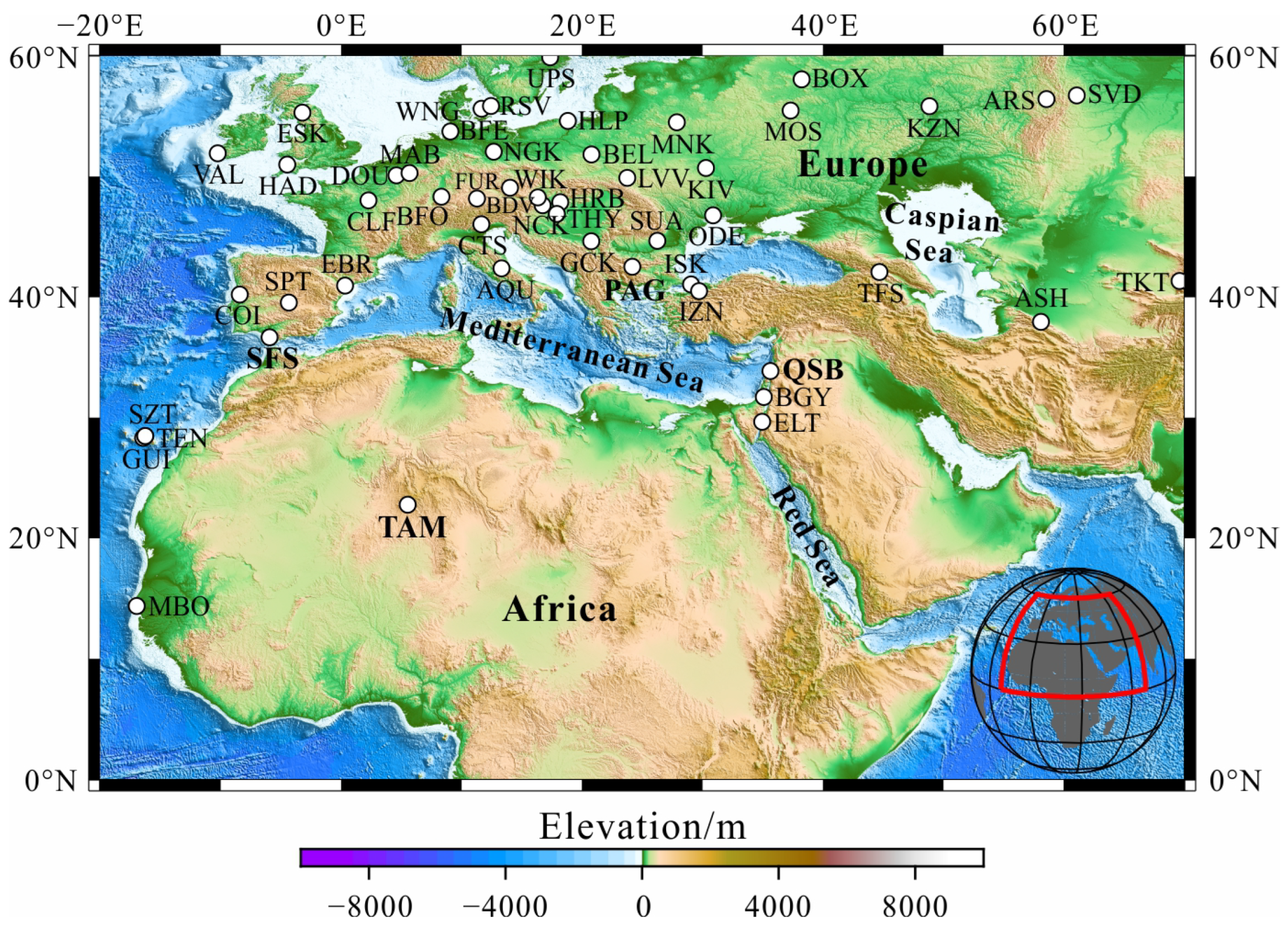
Figure 1. The locations of the selected geomagnetic observatories in North Africa and Southern Europe. White circles indicate the geomagnetic observatories used in the following analysis, and the adjacent abbreviations are the codes of the observatories.
Applsci 13 00689 g001
Figure 2. C-responses at 50 selected observatories; (a,b) are the real and imaginary components of C-responses.
Applsci 13 00689 g002
Figure 3. Electrical conductivity of the shell comprised of oceans and continents used to correct the ocean effect on C-responses and drawn in a geomagnetic coordinate system. White circles represent the used observatories in the geomagnetic coordinate system. The outlines of oceans and continents in a geographic coordinate system are also depicted.
Applsci 13 00689 g003
Figure 4. The one-dimensional (1D) initial model used in this paper.
Applsci 13 00689 g004
Figure 5. Plots of variations in the inversion parameters with iterations. (a) Root–mean–squares (RMS) of data misfit; (b) regularization parameter λ; (c) model roughness; (d) penalty function.
Applsci 13 00689 g005
Figure 6. Fitting curves of the inverted responses and observed data.
Applsci 13 00689 g006
Figure 7. Electrical conductivity model of the mantle beneath North Africa and Southern Europe. σ is the conductivity of the inverted model, and σ 0 is the conductivity of the initial model. (ad) are the electrical conductivity model of depth 250–410 km, 410–520 km, 520–670 km, 670–900 km, respectively. Black arrows and the nearby CAL and HEL are the subducted slabs imaged by seismic tomography [23]. A and B represent Anomaly A and Anomaly B, respectively.
Applsci 13 00689 g007
Figure 8. The resolution kernel checkerboard model in a single layer (a); (b,c) correspond to a single inverse model in which the checkerboard model is within the ranges 520–670 km and 670–900 km. White circles are the locations of geomagnetic observatories and are the same as in Figure 1.
Applsci 13 00689 g008
Figure 9. Curves of fit of the response of re-forward, inverted, and observed data for four geomagnetic observatories (SFS, PAG, TAM, and QSB) distributed around the anomalies. The four stations are marked with bold in Figure 1.
Applsci 13 00689 g009
Figure 10. The conductivity of Anomaly A.
Applsci 13 00689 g010
Figure 11. A rock physics model is used to interpret the conductivity of Anomaly A; (a) is the conductivity of the topmost lower mantle, which varies with temperature, and the normal temperature is approximately 1900 K [42]; (b) is the conductivity of ringwoodite, which varies with temperature and water content in the lower MTZ. The range of Anomaly A is also marked in the figures.
Applsci 13 00689 g011
Table 1. Station details of the observatories used in this article. GM corresponds to the geomagnetic coordinates, and the data length is the duration of the recorded time series geomagnetic field data at the station.
CodeLongLatGM-
Long
GM-
Lat
Data
Length
CodeLongLatGM-
Long
GM-
Lat
Data
Length
AQU42.3813.3242.3994.651960–2009KZN55.8348.8549.8131.711957–2016
ARS56.4358.5749.2140.051973–2018LVV49.923.7547.87107.221957–2019
ASH37.9558.1131.06135.31959–1990MAB50.35.6851.3990.151995–2021
BDV49.0814.0248.7597.731994–2020MBO14.38343.0320.0357.511952–2020
BEL51.8420.7950.24105.271966–2021MNK54.527.8851.62112.911961–2019
BFE55.6211.6755.4398.541981–2008MOS55.4737.3251.08121.681957–2020
BFO48.338.3249.0391.912006–2021NCK47.6316.7246.8899.741993–2021
BGY31.7235.0928.27112.661989–2019NGK52.0712.6851.8697.731932–2021
BOX58.0738.2353.45123.611977–2020ODE46.7830.8843.67112.691957–1991
CLF48.022.2649.7985.791936–2021PAG42.5224.1840.64105.091956–2020
COI40.22351.5844.0971.961964–2021QSB33.8735.6430.29113.652000–2007
CTS46.0511.6546.2494.281996–2020RSV55.8512.4555.5199.41927–1981
DOU50.14.651.38891957–2021SFS36.67354.0640.2173.491957–2021
EBR40.960.3343.2881.331957–2021SPT39.55355.6542.7575.951997–2021
ELT29.6734.9526.28112.091998–2015SUA44.6826.2542.39107.711995–2021
ESK55.31356.7957.7783.611911–2021SVD56.7361.0749.21142.211930–1980
FUR48.1711.2848.3594.731940–2021SZT28.48343.7433.8460.831961–1992
GCK44.6320.7743.28102.532005–2020TAM22.795.5324.681.971993–2021
GUI28.32343.5633.7160.611993–2021TEN28.48343.7433.8460.831961–1992
HAD50.99355.5253.8680.081957–2021TFS42.0944.736.95123.991957–2001
HLP54.6118.8253.23104.711966–2021THY46.917.945.97100.61991–2021
HRB47.8718.1946.86101.231906–2021UPS59.917.3558.5106.332003–2020
ISK41.0629.0638.4109.261950–1999VAL51.93349.7555.7574.531957–2017
IZN40.529.7337.74109.742007–2021WIK48.2716.3247.5799.611955–2015
KIV50.7230.347.58113.541958–2019WNG53.749.0754.0995.081943–2021
Disclaimer/Publisher’s Note: The statements, opinions and data contained in all publications are solely those of the individual author(s) and contributor(s) and not of MDPI and/or the editor(s). MDPI and/or the editor(s) disclaim responsibility for any injury to people or property resulting from any ideas, methods, instructions or products referred to in the content.

