Fault Identification Technology of 66 kV Transmission Lines Based on Fault Feature Matrix and IPSO-WNN

Abstract

Due to the barely resonant earthed system used in the transmission line, it is more challenging to identify faults at a 66 kV voltage level because of insufficient fault identification techniques. In this paper, a 66 kV transmission line fault identification method based on a fault characteristic matrix and an improved particle swarm optimization (IPSO)-wavelet neural network (WNN) is proposed to address the difficulties in extracting and detecting characteristic parameters. The maximum matrix of the dbN wavelet was used to determine its decomposition scale and construct the fault characteristic matrix based on the energy values of frequency bands. The decomposition scale of the dbN wavelet was determined by the modulus maximum matrix to ensure the integrity of fault information. The fault feature matrix was then constructed based on the energy values of frequency bands and the fault feature was accurately extracted. In this research, aiming at the problems such as slow convergence speed and a tendency to fall into local minima, the WNN algorithm is enhanced with the IPSO algorithm. This significantly increased the convergence speed of the identification model and its ability to discover the global optimal solution. The simulation results demonstrate that this method can effectively and accurately identify the fault type with high identification accuracy, quick identification, and robust adaptability. Under challenging working conditions, it is capable of accurately identifying the fault type of 66 kV transmission lines.

1. Introduction

Efficient and accurate fault identification is critical for emergency repair of high voltage transmission lines, which are an integral part of the power system and prone to failure. Compared with traditional transmission lines, 66 kV transmission lines are characterized by high voltage levels, long distances, complex topological structures, large capacitance to the ground during a fault, and a tendency to generate arc over-voltages, which lead to complex fault features and difficulties in accurate extraction and fault identification. During fault events, zero-sequence current and zero-sequence voltage change first and are more accurate, complete, and fault-tolerant than steady-state current and voltage. In the case of high-resistance ground faults, the transient characteristics of fault high-frequency signals are inversely proportional to the transition resistance [1], and the transient zero-sequence current has a nonlinear relationship in the transition process [2,3,4]. Over the years, various fault detection methods based on zero-sequence current and voltage have been developed to detect ground faults, such as one that extracts waveforms based on fault morphological characteristics and another that uses the transient main resonant component [5]. However, these methods have limitations in actual working conditions and can struggle to distinguish the resonant component from the power frequency component. Further, a high-resistance ground fault detection method based on the transient main resonant component has been proposed by Zhang et al. [6], however, this method is not effective at extracting the main resonant component and it is difficult to distinguish the main resonant component from the power frequency component. There are several primary causes of arc ground faults, including lightning impulses, poor connections, and aging insulation [7,8]. However, arc grounding faults cannot be accurately identified. Moreover, a method using the change in waveforms such as voltage-current characteristics and zero-sequence currents as features has been proposed for fault recognition [9]. In addition, a fault identification method based on artificial neural networks has been proposed [10] due to the difficulty in extracting the characteristics of arc earth faults and the differences in fault characteristics at different voltage levels and in different environments. The method requires further consideration to distinguish faults from normal system disturbances. A time-domain analysis method based on Hilbert–Huang transform and a wavelet analysis method based on the time distribution characteristics of fault harmonic characteristics have also been proposed [11,12]. However, these methods only analyze and judge the waveform without extracting and optimizing fault features.

In view of the difficulty of fault feature extraction and fault type identification for 66 kV transmission lines, a fault recognition method based on a fault characteristic matrix and an improved particle swarm optimization (IPSO)-wavelet neural network (WNN) has been proposed in this paper. Firstly, in the aspect of fault feature analysis and extraction, theoretical and simulation analysis is carried out for various types of faults, and fault features are selected as the basis for identification. Secondly, in order to ensure the integrity of fault information, the decomposition scale of dbN wavelet is determined by using the mode maximum matrix, and the fault characteristic matrix is constructed by combining the energy values of each frequency band, so as to achieve accurate fault feature extraction. In view of the limitations of standard WNN, this paper improves a hidden layer of the WNN i to reduce the impact of large fluctuation data on identification accuracy, and an IPSO algorithm is used to design a prediction error function, improving the recognition accuracy and speed of the recognition model, so as to realize the rapid and accurate recognition of fault types. Finally, a large number of simulation results show that the proposed method can realize the fault type identification of 66 kV transmission lines with high recognition accuracy, a fast recognition speed, and strong adaptability.

2. Fault Analysis and Feature Extraction

The failure process of the 66 kV transmission line can be divided into a transient state and a steady state. In the steady state, the system’s zero-sequence current is at a low level due to the arc suppression coil, making it difficult to use for fault identification. In the transient process, the fault transient component is several times higher than the steady component. Therefore, this paper uses fault transient electrical gas to identify a single-phase ground fault, which can be classified into high resistance ground faults and arc ground faults. Metallic ground faults, which are rare, are not considered in this paper.

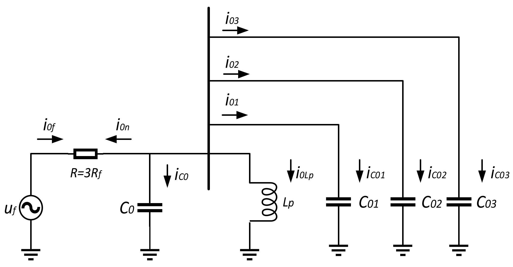
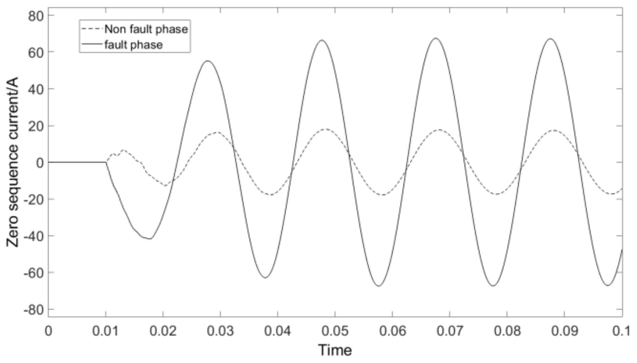
2.1. Single-Phase Ground Fault Simulation and Analysis

Transmission line operating environment is complex and affected by many factors, including non-ideal conductors such as tree branches, sand, and turf, which can cause single-phase ground faults. These faults, caused by high-resistance media, are usually characterized by transition resistance higher than 200 Ω and are collectively referred to as high-resistance ground faults. If not addressed in a timely manner, these faults can expand in scope and seriously affect the stable operation of transmission lines. When a fault occurs, the system’s operation produces high-frequency electromagnetic oscillation, causing line-wide over-voltage for several hours and posing a serious threat to the weak insulation areas of the transmission line.

Since arc ground faults are easy to recognize due to their distinct characteristics and high resistance ground faults and arc ground faults are common and difficult to identify in the actual working conditions of 66 kV transmission lines, this paper focuses on these two types of faults and proposes fault judgment criteria through simulation analysis of various fault types to achieve the goal of fault identification.

2.1.1. High Resistance Ground Fault

When a high resistance ground fault occurs, the fault equivalent circuit is shown in Figure 1. The resistance R can be approximated as 3 times the transition resistance $R_f$. Due to the large value of the transition resistance, the zero-sequence capacitance flowing through the system is small and the transient resonant frequency is low, so the line inductance L can be ignored. The fault transient process is mainly a parallel resonance process between the equivalent inductance $L_p$ of the arc suppression coil and the ground capacitance $C_{0\Sigma }$ of the system.

Figure 1 shows that $C_{0k}\left(k=1,2,3\right)$ is the zero-sequence distributed capacitance of line k to ground, $C_{0\Sigma }={\displaystyle \sum }_{k=1}^3{C}_{0k}$; $i_{0k}$ is zero sequence current of the k feeder, and $i_{C0j}$ is zero sequence capacitance current to ground. $i_{0f}$ and $i_{0L_p}$ are the zero-sequence current at the fault point respectively and $u_f$ is the zero-sequence voltage of the bus.

The second-order nonlinear homogeneous differential equation is given in Equation (1):

$$3R_f{C}_{0\Sigma }{L}_p\frac{d^2{i}_{0L_p}}{d{t}^2}+L_p\frac{d{i}_{0L_p}}{dt}+3R_f{i}_{0L_p}=u_f\left(t\right)$$

(1)

The characteristic roots of this differential equation are given in Equation (2):

$$\left\{\begin{array}{l}{p}_1=-\frac{1}{6R_f{C}_{0\Sigma }}+\sqrt{{\left(\left(\frac{1}{6R_f{C}_{0\Sigma }}\right)\right)}^2-\frac{1}{L_p{C}_{0\Sigma }}}\hfill \\ p_2=-\frac{1}{6R_f{C}_{0\Sigma }}-\sqrt{{\left(\frac{1}{6R_f{C}_{0\Sigma }}\right)}^2-\frac{1}{L_p{C}_{0\Sigma }}}\hfill \end{array}\right.$$

(2)

The zero-sequence current flowing through the arc suppression coil is given in Equation (3):

$$i_{0L_p}\left(t\right)=Bsin\left({\omega }_{0}t+{\phi }_2\right)+A_1{e}^{p_{1}t}+A_2{e}^{p_{2}t}$$

(3)

Here, ${\omega }_0$ is the angular frequency of zero-sequence current oscillation, and $B,A_1,A_2, and {\phi }_2$ has the following meanings (Equation (4)):

$$\left\{\begin{array}{c}B=\frac{U_m}{\sqrt{{\left(3R_f\right)}^2{\left(1-{\omega }_0^2{L}_p{C}_0\right)}^2+{\left({\omega }_0^2{L}_p\right)}^2}}\\ A_1=\frac{{\omega }_{0}Bcos{\phi }_2-p_{2}Bsin{\phi }_2}{p_2-p_1}\\ A_2=\frac{{\omega }_{0}Bcos{\phi }_2-p_{1}Bsin{\phi }_2}{p_2-p_1}\\ {\phi }_2=\theta -arctan\frac{{\omega }_0{L}_p}{3R_f\left(1-{\omega }_0^2{L}_p{C}_0\right)}\end{array}\right.$$

(4)

According to Equation (4), busbar zero sequence voltage is given in Equation (5):

$$u_0\left(t\right)=L_p\frac{d{i}_{0L_p}}{dt}={\omega }_0{L}_{p}Bcos\left({\omega }_{0}t+{\phi }_2\right)+L_p{p}_1{A}_1{e}^{p_{1}t}+L_p{p}_2{A}_2{e}^{p_{2}t}$$

(5)

The zero-sequence capacitance to the earth is given in Equation (6):

$$i_{C0k}=C_{0k}\frac{d{u}_0}{dt}={\omega }_0^2{L}_p{C}_{0k}Bsin\left({\omega }_{0}t+{\phi }_2\right)+ L_p{C}_{0k}\left(p_1^2{A}_1{e}^{p_{1}t}+p_2^2{A}_2{e}^{p_{2}t}\right)$$

(6)

The zero-sequence current at the fault point is given in Equation (7):

$$i_{0f}=i_{0L_p}+i_0=\left(1-{\omega }_0^2{L}_p{C}_0\right)Bsin\left({\omega }_{0}t+{\phi }_2\right)+\left[L_p{C}_0{p}_2^2+1\right]A_1{e}^{p_{1}t}+\left[L_p{C}_0{p}_2^2+1\right]A_2{e}^{p_{2}t}$$

(7)

According to Equation (7), each outgoing zero-sequence current consists of a steady-state component and a transient component. Considering that the initial value of the two-phase attenuated DC component is not 0 at the same time and the attenuation factors are not equal, the transient-free component always exists. The grounding resistance value is proportional to the transient duration, which is helpful for fault diagnosis.

For high-resistance ground faults, the greater the ground resistance, the lower the zero-sequence current flowing through the system, and the charge and discharge speed of the zero-sequence capacitor on the line is slow, resulting in a low transient resonant frequency of the system. In this case, the inductive reactance of the circuit is low and can be essentially ignored. The transition process occurs through a parallel connection between the zero-sequence capacitance and arc suppression inductance. Additionally, the transition resistance is inversely proportional to the zero-sequence current at the fault point and directly proportional to the transient resonant frequency. The maximum resonance frequency only slightly exceeds the power frequency and in this case, the resonance frequency approaches the power frequency, the waveform of the zero-sequence current exhibits beat frequency phenomena.

As an example, consider a high resistance ground fault with a ground resistance of 1000 Ω that occurs 1 km from phase A of fault line 3 at 0.01 s. The zero-sequence current of the fault line and non-fault phase is shown in Figure 2.

Simulated results indicate that in the high-resistance earth fault state, the first half wave phase of the fault phase is the opposite, and the wave’s amplitude differs greatly from that of the non-fault phase. A high transition resistance results in a resonance frequency that is virtually the same as a working frequency, and a zero-sequence current oscillation frequency that is certain, but there is a phenomenon known as the beat frequency at the outer edge of each wave peak, resulting in a waveform with a longer wavelength.

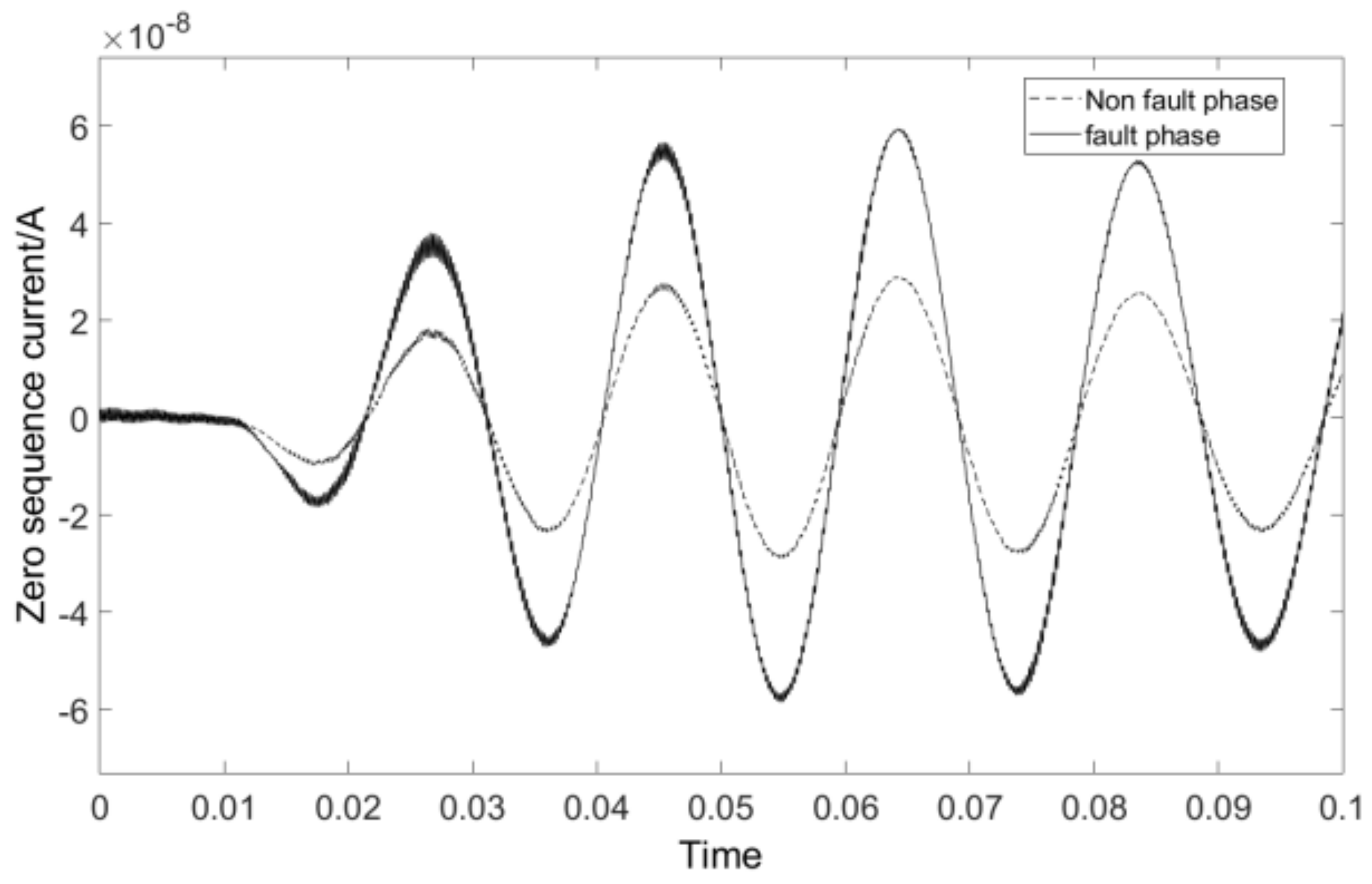
2.1.2. Arc Ground Fault

Arc ground fault is a common and harmful fault that is difficult to detect due to its complex mechanism and difficulty in extracting fault characteristics. In order to address these problems, this paper analyzes the transient electrical volume when simulating arc generation and arc grounding fault, and proposes an identification basis.

(1.)

Mayr arc model

Mayr arc is selected for research in this paper, and the Mayr arc simulation model is built through MATLAB/simulation combined with the arc, as highlighted in Equation (8):

$$\frac{1}{g}\left(\frac{dg}{dt}\right)=\frac{1}{{\tau }_M}\left(\frac{ei}{p_{loss}}-1\right)=\frac{1}{{\tau }_M}\left(\frac{ei}{e_{0}i}-1\right)$$

(8)

In the formula, the expression of each parameter is given in Equation (9):

$$\left\{\begin{array}{c}\hspace{1em}g=g_0{e}^{\frac{Q}{Q_0}}\\ \tau =f\left(g,\frac{dg}{dt},p_{loss}\right)=\frac{g\cdot \frac{dg}{dt}}{p_{loss}}\\ {\tau }_M=g\cdot \frac{Q_0}{g}\cdot \frac{1}{p_{loss}}=\frac{Q_0}{p_{loss}}\\ p_{loss}=p_{cd}+p_{d1}+p_{fs}\end{array}\right.$$

(9)

where $p_{loss}$ is the total arc energy loss, p_cd is transmitted and distributed power, $p_{d1}$ is convective emission power, $p_{fs}$ is radiation emission power;$g$ is a constant; and $Q_0$ is heat per arc column.

(2.)

Simulation of Arc ground failure

Arc earthed failure not only has a great impact on the normal operation of the line, but also reduces the insulation level of the whole line. Figure 3 and Figure 4 show the arc current voltage waveform, respectively.

The voltage waveform of the arc has serious distortion and presents nonlinear characteristics, as can be seen in Figure 4 and Figure 5. The arc starting voltage rises rapidly and then falls off immediately. The voltage crosses zero after a period of constant voltage, then turns to arc extinguishing voltage. The current waveform can be regarded as sine wave. When the arc current is close to zero, the current changes slowly and exhibits a “resting zero” phenomenon. After the “resting zero”, the current changes faster than a sine wave, demonstrating the effectiveness of the model.

The zero-sequence currents under fault and non-fault conditions are shown in Figure 5. As can be seen in Figure 6, when an arc-earthed failure occurs, the suppression of arc coils is effective. The phase of the first-half wave of zero-sequence current of the fault line in the transient process is opposite to that of the non-fault line, that is, the phase difference is 180°. In the steady-state process, the zero-sequence current has no phase difference; the fault’s zero-sequence current has a large amplitude, so it is a good indicator of the arc grounding fault.

2.2. Short Circuit Fault Analysis and Characteristic Diagnosis

Short-circuit faults are more common in power system faults, which can be divided into phase-to-phase short circuit faults and three-phase short circuit faults. In this paper, the fault characteristics and judgment basis of short-circuit fault are analyzed through simulations.

When an A or B phase-to-phase short-circuit fault occurs on the line, the fault current is shown in Figure 6. In the case of a phase-to-phase short circuit fault, the fault current of the fault phases A and B of the transmission line suddenly increases several times, with a large fluctuation range, which can be used as a basis for judgment.

In the three-phase short-circuit state, the current waveform of each line is shown in Figure 7, and the zero-sequence current of the fault line and non-fault line is shown in Figure 8.

When a three-phase short-circuit fault occurs, the three-phase current of A, B, and C suddenly increases several times at the fault moment, while the increase of transient zero-sequence current is substantially limited in the transient process, making it difficult to serve as a basis for judgment. Therefore, this paper concludes that the short-circuit fault type can be judged by the increase in the number of phases through the fault phase current.

3. Fault Feature Extraction

This paper employs wavelet transform to decompose fault zero sequence current signal since it has good processing effects on abrupt and nonlinear signals. To ensure the integrity of fault information after decomposition, this paper determines the decomposition scale using the modular maximum matrix, combined with an energy value equation to calculate the energy value of each frequency band and build a fault characteristic matrix, which can represent the characteristics of different types of faults, providing significant support for the accurate identification of faults.

3.1. Selection of Basic Parameters

3.1.1. The Selection of Wavelet Basis Function

There are several kinds of wavelet basis functions, and different wavelet basis functions have varying analysis effects. The commonly used wavelet basis functions include Gaus, Dmey, Haar, and dbN. In order to realize the transient feature extraction of phase current and zero-sequence current, dbN is selected as the wavelet basis function in this paper. The advantage of this is that the localization of the frequency domain increases with an increase in N. In practical application, DB analysis has good performance. Extensive test results show that DB6 provides best performance, so it is chosen in this paper.

3.1.2. Decomposition Scale and Selection of Characteristic Quantities

A wavelet function has the advantage of being able to extract the signal mutation location from the maximum value of the pair of modes as a result of its small scale, but its disadvantage is its sensitivity to noise and inability to extract the fault position accurately. When the decomposition scale is large, harmonic interference can be prevented, but the position of the maximum modulus and the signal mutation point cannot coincide effectively, so it is highly important to choose the appropriate decomposition scale.

In this paper, a maximum modulus matrix $A_{ij}$ is established to help determine the decomposition scale, where i represents the fault line and j represents the decomposition scale. The maximum modulus matrix is established as shown in Equation (10).

$${{\displaystyle A}}_{ij}=\left[\begin{array}{c}{a}_{11}\hspace{1em}{a}_{12}\hspace{1em}{a}_{13}\hspace{1em}{a}_{14}\hspace{1em}{a}_{15}\hspace{1em}{a}_{16}\\ a_{21}\hspace{1em}{a}_{22}\hspace{1em}{a}_{23}\hspace{1em}{a}_{24}\hspace{1em}{a}_{25}\hspace{1em}{a}_{26}\\ a_{31}\hspace{1em}{a}_{32}\hspace{1em}{a}_{33}\hspace{1em}{a}_{34}\hspace{1em}{a}_{35}\hspace{1em}{a}_{36}\end{array}\right]$$

(10)

After the decomposition scale is determined, the energy value of the corresponding characteristic frequency band is calculated using Equation (11).

$$E_{6,J}={{\displaystyle \int }}_{-\infty }^{+\infty }\left|S_{6,J}\left(t\right)\right|dt={\displaystyle \sum }_{k=1}^n{\left|d_{j,k}\right|}^2$$

(11)

The frequency band energy corresponding to the zero-sequence current of each circuit is calculated using Equation (11), and the maximum energy value in each frequency band is selected to form a characteristic matrix. Through the analysis of the training model, fault type identification and diagnosis are achieved. The characteristic matrix $B_{cd}$ is shown in Equation (12).

$${{\displaystyle B}}_{cd}=\left[\begin{array}{c}{b}_{11}\hspace{1em}{b}_{12}\hspace{1em}{b}_{13}\hspace{1em}{b}_{14}\hspace{1em}{b}_{15}\hspace{1em}{b}_{16}\\ b_{21}\hspace{1em}{b}_{22}\hspace{1em}{b}_{23}\hspace{1em}{b}_{24}\hspace{1em}{b}_{25}\hspace{1em}{b}_{26}\\ b_{31}\hspace{1em}{b}_{32}\hspace{1em}{b}_{33}\hspace{1em}{b}_{34}\hspace{1em}{b}_{35}\hspace{1em}{b}_{36}\end{array}\right]$$

(12)

where c is the number of lines and d is the decomposition scale.

3.2. Calculation of Fault Characteristic Matrix

In this paper, the maximum modulus matrix is obtained by db6 decomposition of the zero-sequence current obtained through fault simulation. Since the simulation model selected in this paper has three lines, $i=3$, and 6 times wavelet decomposition $j=6$, the maximum matrix of high resistance grounding fault mode is $A_{36}$.

$$A_{36}=\left[\begin{array}{c}0.0033\hspace{1em}-0.0213\hspace{1em} -0.0601\hspace{1em}0.2109\hspace{1em}-0.1955\hspace{1em}0.2451\\ 0.00334\hspace{1em}0.0026\hspace{1em} -0.0732\hspace{1em}0.1324\hspace{1em} 0.1465\hspace{1em} 0.2652\hfill \\ 0.0092\hspace{1em}-0.0597\hspace{1em} 0.0668\hspace{1em}-0.4361\hspace{1em} 0.1872\hspace{1em}-0.5461\end{array}\right]$$

According to matrix $A_{36}$, the largest elements of high-resistance grounding fault mode are all in the sixth column, namely db6 scale, and the corresponding system decomposition scales of the three lines are consistent. According to Equation (12), energy values are constructed to realize feature extraction of high-resistance grounding fault.

$$B_{36}=\left[\begin{array}{c} 0.71\hspace{1em} 0.62\hspace{1em}-0.75\hspace{1em}-0.76\hspace{1em}0.81\hspace{1em}0.01\\ 0.64\hspace{1em} 0.57\hspace{1em}-0.83\hspace{1em}-0.84\hspace{1em}0.78\hspace{1em}0.01\\ -1.23\hspace{1em}1.87\hspace{1em}-2.04\hspace{1em}-2.56\hspace{1em}2.85\hspace{1em}0.01\end{array}\right]$$

It can be seen from the characteristic matrix $B_{63}$ that the characteristic quantity of the fault line is greater than that of the non-fault line, and the characteristic quantity of each scale gradually increases. The first column element of the faulty line is also different from that of the non-faulty line, which conforms to the characteristics of high-resistance earthed fault proposed above.

Maximum matrix of arc ground fault matrix $A_{36}$ is:

$$A_{36}=\left[\begin{array}{c}-0.05\hspace{1em}0.23\hspace{1em}-0.52\hspace{1em} 1.64\hspace{1em} 0.56\hspace{1em} 0.47\hfill \\ 0.04\hspace{1em}-0.24\hspace{1em}1.55\hspace{1em} 5.37\hspace{1em} -2.54\hspace{1em} 1.59\hfill \\ 0.17\hspace{1em} 0.68\hspace{1em} 3.56\hspace{1em}-14.66\hspace{1em}-6.23\hspace{1em}-9.53\end{array}\right]$$

It can be seen from matrix $A_{36}$ that the largest elements of the high-resistance grounding fault mode are all in the fourth column, namely db4 scale. The characteristic matrix of the corresponding decomposition scale is constructed as follows:

$$B_{34}=\left[\begin{array}{c} 1.38\hspace{1em}-1.02\hspace{1em} 0.67\hspace{1em} 0.37\hspace{1em}0.53\hspace{1em}-0.51\hfill \\ 1.42\hspace{1em}-0.98\hspace{1em} 0.72\hspace{1em} 0.31\hspace{1em}0.46\hspace{1em}-0.56\hfill \\ -3.56\hspace{1em}1.39\hspace{1em}-2.13\hspace{1em}3.24\hspace{1em}1.53\hspace{1em}-1.43\end{array}\right]$$

According to the characteristic matrix, the characteristic quantity of fault line is larger than that of the other lines and the polarity is opposite, which conforms to the characteristics of an arc ground fault proposed above.

4. Fault Identification Method Based on IPSO-WNN

WNN is a type of neural network that uses an excitation function error back propagation and wavelet cardinality as the hidden layer node. This paper chooses wavelet neural network to realize fault identification because it fully combines the good time-frequency localization property of wavelet transform and the self-learning property of neural network.

4.1. WNN Hidden Layer Output Optimization

The standard WNN structure diagram is shown in Figure 9.

In Figure 9, X and Y denote input samples and predicted outputs; ${\omega }_{ij}$ are the weights connecting output layer node $\mathrm{i}$ and implicit layer node $j$;${\omega }_{ik}$ is the weight connecting node $j$ in the implicit layer and node $k$ in the output layer; and $\psi \left(x\right)$ is the dbN function.

There are n input nodes in WNN. The input sequence $X=\left(x_1,x_2,\dots ,x_n\right)$ is processed by the dbN function and the output value is obtained in the hidden layer.

The calculated values of the standard WNN implied layer are susceptible to the influence of the input layer data, with large fluctuations between values and a single calculation method, which cannot meet the requirements of this paper for fault identification accuracy. Therefore, using quantified connection weights between input and implied layers, this paper seeks to reduce the influence of single input data. The calculation is shown in Equation (13):

$$u_j=\psi \left[\frac{{\sum }_{i=1}^n{\omega }_{ij}{x}_i-b_j}{a_j}\right],j=1,2,3,\dots ,l$$

(13)

where $u$ is the output value of the implicit layer nodes, $n$ is the number of nodes in the input layer, and $l$ is the number of implied layers, and $a,b$ denote the scaling factor and translation factor of the dbN function, respectively.

After the implicit layer processing, the output value obtained is given in Equation (14).

$$y_k={\sum }_{j=1}^l{\omega }_{jk}{u}_j,k=1,2,3,\dots ,m$$

(14)

where $y_k$ is the actual output of the network, and $m$ is the number of output layer nodes.

The error function of WNN is usually expressed as the mean squared difference between the actual output value and the desired output value, as shown in Equation (15).

$$E_D={\sum }_{k=1}^m(y_k-\widehat{y_k}{)}^2$$

(15)

where $E_D$ is the training error, and $\widehat{y_k}$ is the desired output.

4.2. Fault Identification Method Based on IPSO-WNN

In order to reduce the prediction error, the mean squared error function in Equation (15) is used as the fitness function of the IPSO algorithm in this paper. Whenever the fitted value is near the actual value, the recognition model error is smaller, and the particle’s fitness is higher, and the current particle is in the best position when the recognition error reaches the expected value.

This paper improves PSO algorithm to make the global search ability and local search ability in a balanced state by acquiring a faster convergence speed and making the algorithm more resistant to falling into local minima.

$$w_i=w_{max}-\frac{i\left(w_{max}-w_{min}\right)}{I_{max}}$$

(16)

where $w_{max}$, $w_{min}$ are the maximum and minimum values of inertia weights, respectively. $I_{max}$ is the preset maximum number of iterations. $w$ is the number of iterations with $I$ linearly decreasing, but to consider the effects of the evolutionary speed and aggregation degree of the particle population, a nonlinear decreasing strategy of inertia weights is proposed in this paper, as given in Equation (17).

$$w_i=\left\{\begin{array}{l}{w}_{max},f\ge f_{avg}\hfill \\ w_{min}+\frac{w_{max}{w}_{min}}{1+e^{favg-f}},f<f_{avg}\hfill \end{array}\right.$$

(17)

where $f$ is the fitness of the particle, $f_{avg}$ is the average fitness of all particles. This method adjusts the inertia weights of the particles based on the relationship between f and $f_{avg}$ in order to enhance the ability of the particles to find the global optimal solution.

The learning factors $c_1$ and $c_2$ in PSO algorithm affect the superiority seeking ability of particles and the information interaction ability between particles. In the standard PSO algorithm $c_1$, and $c_2$ are equal fixed values, which have a large impact on the convergence speed and the merit-seeking ability of the algorithm. Therefore, in this paper, the learning factor is optimized based on the nonlinear decreasing strategy for the inertial weight.

$$\left\{\begin{array}{c}{c}_1\left(t\right)=2-e^{g_t-\frac{1}{N}{\sum }_{i=1}^N{p}_i}\\ c_2\left(t\right)=2-c_1\left(t\right)\end{array}\right.$$

(18)

where N is the total number of particles, $c_1$ is the number of particles in the first $t$ at the second iteration, and $c_2$ is the value of $g_t$, which is the optimal solution of the current particle swarm. $p_i$ is the optimal solution of the first $i$ optimal solution of the first i particle.

From Equation (18), it can be seen that as the iterations proceed, the learning factor $c_1$ decreases nonlinearly and $c_2$ nonlinearly increases, which significantly increases the convergence speed of the algorithm and achieves the goal of enhancing the algorithm’s ability to find the global optimal solution.

4.3. Fault Identification Process

Through the analysis of the expected output, fault data and the fault features of each fault type are input into the diagnosis model for training. The model training input values are shown in

Table 1. Model training input values.

Input Fault Type	Input Fault Characteristics	Desired Output
Three phase short circuit fault	$\Delta I$ > 100 and $\Delta I_{\mathrm{i}}$(i = A, B, C) > 100A is l, l = 2	1
High resistance ground fault	$\Delta I$ > 100 and l = 3	2
Arc earthed failure	$U_0>0.15U_n$ and $B_{cd}$	3
Three phase short circuit fault	$U_0>0.15U_n$ and $B_{cd}$	4

.

In Table 1, $U_0$ represents the zero-sequence voltage and $U_n$ represents phase voltage of the line. When a single-phase grounding fault occurs on the line, it conforms to $U_0>0.15U_n$, which can be used as the basis for determining the grounding fault.

The fault identification based on IPSO-WNN is shown in Figure 10.

5. Simulation Verification

In this section, the feature values corresponding to each fault type are input to the fault diagnosis model for verification, and the prediction error is reduced by setting the number of implied layers and the number of iterations. The optimal choice is achieved when the number of implied layers is 50 and the number of iterations is 2000, as demonstrated by a large number of simulations. By combining etime() and clock in MATLAB, the time difference between $t_1$ and $t_0$ in Figure 10 is calculated as the fault identification time. This paper uses the same experimental equipment, in the same data volume environment, in order to reduce the error in computing time brought by the computer hardware.

To further verify the applicability of the method proposed in this paper, comparison experiments were conducted by setting different fault distances and different fault initial phase angles, and the experimental results are shown in

Table 2. Fault distances.

Number of Training Samples	Number of Test Samples	Fault Distance/km	Recognition Accuracy/%	Training Time/s
150	50	5	98	134
		20	96	148
		40	96	167
		60	94	181

and

Table 3. Different fault initial phase angles.

Number of Training Samples	Number of Test Samples	Fault Initial Phase Angle/°	Recognition Accuracy/%	Training Time/s
150	50	0	96	171
		25	96	159
		45	98	146
		60	96	157
		90	100	143

.

According to Table 2, the fault identification accuracy decreases with the increase of the fault distance. When the fault distance is 60 km, the fault identification accuracy is 96% and the fault identification time is 181 s, which verifies the strong applicability and robustness of IPSO-WNN under different fault distances.

In Table 3, it is evident that IPSO-WNN is equally applicable at different initial fault phase angles.

In this paper, the recognition accuracy and recognition time of IPSO-WNN are compared with the currently used recognition methods: WNN, support vector machine (SVM), PSO–WNN, and SSA–SVM. The comparison results are shown in

Table 4. Comparison of the performance of different methods.

Number of Training Samples	Number of Test Samples	Algorithm Type	Recognition Accuracy/%	Training Time/s
150	50	WNN	82	1149
		SVM	84	921
		PSO-WNN	94	547
		SSA-SVM	92	344
		IPSO-WNN	98	164

.

Table 4 shows that IPSO-WNN has superior recognition accuracy and recognition time as compared to other algorithms, proving the superiority of the proposed method.

In summary, this paper presents a method for identifying various types of transmission line faults using IPSO-WNN, which combines the time-frequency localization property of wavelet transform with the self-learning ability of neural networks. The method is verified through comparison experiments with different identification methods, different fault distances, and different fault initial phase angles. The results show that the proposed method has a high identification accuracy and a fast identification speed, which can meet the needs of actual working conditions. Overall, the proposed IPSO-WNN method is a promising approach for fault identification in transmission lines.

6. Conclusions

In this paper, the fault characteristics of different fault types of 66 kV transmission lines were simulated and analyzed. The decomposition scale of the dbN wavelet was determined using the mode maximum matrix to ensure the integrity of fault information. A fault characteristic matrix, which characterizes the fault characteristics based on the energy value of each frequency band, was also proposed. This laid a solid foundation for the subsequent fault identification. As for the fault identification model, the standard WNN algorithm’s hidden layer was improved to weaken the influence of data with large fluctuations on the identification accuracy. The prediction error function was improved by combining it with the IPSO algorithm, greatly improving the convergence speed of the identification model and its ability to find the global optimal solution. Finally, the superiority and applicability of the method were further verified through comparison experiments, demonstrating its ability to meet the needs of actual working conditions and complex environments.

References

1. Lukowicz, M.; Solak, K.; Wiecha, B. Optimized bandpass admittance criteria for earth fault protection of MV distribution networks. Int. J. Electr. Power Energy Syst. 2020, 119, 105855. [Google Scholar] [CrossRef]
2. Abdollahzadeh, H. A new approach to eliminate impacts of high-resistance faults by compensation of traditional distance relays’ input signals. Electr. Power Syst. Res. 2021, 194, 107098. [Google Scholar] [CrossRef]
3. Li, B.; Wang, W.; Wen, W.; Yao, B.; He, J.; Wang, X. Unbalanced currents of EHV multi-circuit lines and coordination of zero-sequence overcurrent relayings. Int. J. Electr. Power Energy Syst. 2021, 126, 106607. [Google Scholar] [CrossRef]
4. Wang, X.; Liu, W.; Liang, Z.; Guo, L.; Du, H.; Gao, J.; Li, C. Faulty feeder detection based on the integrated inner product under high impedance fault for small resistance to ground systems. Int. J. Electr. Power Energy Syst. 2022, 140, 108078. [Google Scholar] [CrossRef]
5. Esmail, E.M.; Elgamasy, M.M.; Kawady, T.A.; Taalab, A.M.I.; Elkalashy, N.I.; Elsadd, M.A. Detection and experimental investigation of open conductor and single-phase earth return faults in distribution systems. Int. J. Electr. Power Energy Syst. 2022, 140, 108089. [Google Scholar] [CrossRef]
6. Zhang, Y.; Wang, X.; Li, J.; Xu, Y.; Wu, G. Small-current grounding fault location method based on transient main resonance frequency analysis. Glob. Energy Interconnect. 2020, 3, 324–334. [Google Scholar] [CrossRef]
7. Gaur, V.K.; Bhalja, B.R.; Saber, A. New ground fault location method for three-terminal transmission line using unsynchronized current measurements. Int. J. Electr. Power Energy Syst. 2022, 135, 107513. [Google Scholar] [CrossRef]
8. El-Naily, N.; Saad, S.M.; Elhaffar, A.; Zarour, E.; Alasali, F. Innovative Adaptive Protection Approach to Maximize the Security and Performance of Phase/Earth Overcurrent Relay for Microgrid Considering Earth Fault Scenarios. Electr. Power Syst. Res. 2022, 206, 107844. [Google Scholar] [CrossRef]
9. Li, J.; Li, Y.; Wang, Y.; Song, J. Single-phase-to-ground fault protection based on zero-sequence current ratio coefficient for low-resistance grounding distribution network. Glob. Energy Interconnect. 2021, 4, 564–575. [Google Scholar] [CrossRef]
10. Arranz, R.; Paredes, A.; Rodríguez, A.; Muñoz, F. Fault location in transmission system based on transient recovery voltage using Stockwell transform and artificial neural networks. Electr. Power Syst. Res. 2021, 201, 107569. [Google Scholar] [CrossRef]
11. Mou, H.; Hu, Z.; Gao, M. New method of measuring the zero-sequence distributed parameters of non-full-line parallel four-circuit transmission lines. Int. J. Electr. Power Energy Syst. 2022, 139, 108040. [Google Scholar] [CrossRef]
12. Lopes, G.N.; Menezes, T.S.; Santos, G.G.; Trondoli, L.H.P.C.; Vieira, J.C.M. High impedance fault detection based on harmonic energy variation via S-transform. Int. J. Electr. Power Energy Syst. 2022, 136, 107681. [Google Scholar] [CrossRef]
Figure 1. High-resistance ground fault equivalent circuit.
Applsci 13 01220 g001
Figure 2. Zero-sequence current of High-resistance ground fault line and non-fault line.
Applsci 13 01220 g002
Figure 3. Arc voltage waveform.
Applsci 13 01220 g003
Figure 4. Arc current waveform.
Applsci 13 01220 g004
Figure 5. Waveform of zero-sequence current in fault phase and non-fault phase of arc grounding fault.
Applsci 13 01220 g005
Figure 6. Phase-to-phase short circuit fault current.
Applsci 13 01220 g006
Figure 7. Three-phase short circuit fault phase current.
Applsci 13 01220 g007
Figure 8. Zero-sequence current.
Applsci 13 01220 g008
Figure 9. The topology of WNN.
Applsci 13 01220 g009
Figure 10. Fault identification based on IPSO-WNN.
Applsci 13 01220 g010