Large-Scale Cluster Parallel Strategy for Regularized Lattice Boltzmann Method with Sub-Grid Scale Model in Large Eddy Simulation

Abstract

As an improved method of the lattice Boltzmann method (LBM), the regularized lattice Boltzmann method (RLBM) has been widely used to simulate fluid flow. For solving high Reynolds number problems, large eddy simulation (LES) and RLBM can be combined. The computation of fluid flow problems often requires a large number of computational grids and large-scale parallel clusters. Therefore, the high scalability parallel algorithm of RLBM with LES on a large-scale cluster has been proposed in this paper. The proposed parallel algorithm can solve complex flow problems with large-scale Cartesian grids and high Reynolds numbers. In order to achieve computational load balancing, the domain decomposition method (DDM) has been used in large-scale mesh generation. Three mesh generation strategies are adopted, namely 1D, 2D and 3D. Then, the buffer on the grid interface is introduced and the corresponding 1D, 2D and 3D parallel data exchange strategies are proposed. For the 3D lid-driven cavity flow and incompressible flow around a sphere under a high Reynolds number, the given parallel algorithm is analyzed in detail. Experimental results show that the proposed parallel algorithm has a high scalability and accuracy on hundreds of thousands of cores.

1. Introduction

Over the past several decades, computational fluid dynamics (CFD) have undergone significant development in numerical simulations of both incompressible and compressible flows. Great progress has been achieved in CFD through the finite difference method [1], finite volume method [2], finite element method [3], and spectral method [4]. The applications of CFD have achieved great success in various fields; magnetized-nanofluid [5,6], nonlinear mixed convection [7,8,9], molecular dynamics [10], cellular automata [11] and others have contributed to these developments. In the past few decades, as a mesoscopic CFD method, the lattice Boltzmann method (LBM) has emerged as an intriguing alternative in CFD for simulating fluid flow [12,13,14,15,16,17,18]. Due to its granular nature and local dynamics, LBM offers several advantages over traditional CFD methods, especially when dealing with complex boundary conditions and parallelization requirements. Its notable feature lies in its suitability for parallel computing, facilitated by localized communication and inherent additivity schemes in numerical operations.

LBM can be flexibly combined with some existing models to solve CFD numerical simulation problems for different situations. In recent years, the Immersed Boundary technique has been seamlessly integrated with LBM, enhancing its capabilities in simulating complex geometries and interactions [19]. By incorporating the Immersed Boundary technique, LBM becomes particularly adept at handling scenarios involving non-circular particles in an enclosure, where a pulsatile flow acts as a counter-flow [20].

Among the many popular LBM models, the single-relaxation-time LBM (SRT-LBM) model [21,22,23] is widely used due to its simplicity and ease of implementation. However, previous studies have revealed that the SRT-LBM model can become numerically unstable when simulating fluids with high Reynolds numbers [24]. To address this issue, one approach suggested for enhancing numerical stability is the introduction of a regularization procedure, which is executed prior to particle collision [25]. This regularization procedure restores certain symmetry properties that might not be inherently satisfied in numerical simulations, leading to higher stability. In addition, the regularized lattice Boltzmann method (RLBM) maintains the simplicity and computational efficiency of the SRT-LBM method while significantly improving the numerical stability.

Large Eddy Simulation (LES) is a pivotal numerical simulation method widely utilized in CFD to investigate turbulent motion. Initially proposed by Smagorinsky in 1963 [26], LES has evolved as an effective tool for studying turbulence across various engineering applications. Its integration with LBM has further enhanced its applicability. In LES, the large turbulent structures are directly resolved, while the smaller ones are modeled, making it computationally efficient for turbulent flow simulations. The method has gained prominence due to the advancement in computational resources and techniques, enabling accurate predictions of complex flow behaviors.

In recent years, researchers have focused on combining LES with LBM, enhancing the simulation capabilities. Hou et al. successfully integrated the Smagorinsky model with Single-Relaxation-Time LBM (SRT-LBM) [27], and Tiftikci et al. introduced the Smagorinsky model into RLBM [28]. By incorporating the Smagorinsky model with RLBM, these approaches have achieved improved accuracy in capturing turbulent phenomena. Notably, the advantage of incorporating the Smagorinsky model in RLBM lies in its completely local computation, preserving the parallel nature of RLBM simulations. This integration signifies a significant advancement in simulating turbulence, enabling researchers to delve deeper into intricate flow dynamics with enhanced precision and computational efficiency.

Since the LES problems handled by RLBM are often large in scale, computing platforms are often required to have high computing power and large storage space. Currently, servers [29] and supercomputers [30] with multicore systems are the first choice for solving LES problems using RLBM in computational fluid dynamics. These computational platforms offer high computing power and ample storage space, which are essential for tackling the large-scale LES problems. As fluid mechanics and artificial intelligence continue to integrate deeply [31,32,33,34,35,36,37,38,39,40], a new computing model is anticipated in the future. However, the current situation is that reliance on the use of servers and supercomputers based on multi-core architectures for solving LES with RLBM still performs much better than AI solutions. It is imperative to employ parallel computing strategies to efficiently address these computational challenges in the realm of handling LES problems by RLBM.

The high-performance computing (HPC) platform provides for the large amount of computational resources required during LES simulation. RLBM needs to design parallel algorithms and formulate computational domain division strategies according to its own characteristics when solving LES simulation. Due to the local dynamics of RLBM with LES (RLBM-LES), DDM can be used to achieve parallelism. Related studies have been presented. Xu et al. [41] used the domain decomposition method to simulate the 3D incompressible flow past a sphere on multi-GPUs. MPI is the optimum solution for implementing computation across compute nodes in HPC. Abas et al. [42] used MPI to accelerate the RLBM simulation implemented on top of the Palabos [43] library, but they only gave performance results and did not show the details on the parallel algorithm. Zavodszky and Paal [44] used RLBM to simulated 3D transient flows in complex geometries on 128 CPU cores but did not provide a performance analysis. Basha and Sidik [45] used the RLBM method to simulate incompressible laminar convection in 2D and 3D channels and the domain decomposition method to parallelize uniform lattice grids, while also providing a performance analysis on a HPC cluster with 32 nodes.

On the one hand, there is no research on the scalability of RLBM-LES on large-scale cluster; on the other hand, parallel algorithms of RLBM only evaluate its parallel performance and still lack practical applications which have no Cartesian grid generation algorithms. Therefore, this paper proposes a parallel algorithm for RLBM to solve LES simulations. The algorithm is based on Cartesian grid generation, domain decomposition method and data exchange strategy on clusters, which empowers RLBM to solve LES with HPC clusters. The scalability of the algorithm on large-scale clusters is also investigated.

The rest of the paper is arranged as follows. Section 2 introduces RLBM-LES and the processing method of the boundary. Section 3 illustrates RLBM-LES parallel implementation. Next, the experimental results are shown and discussed in Section 4. Finally, Section 5 summarizes this paper.

2. RLBM-LES and Boundary Condition

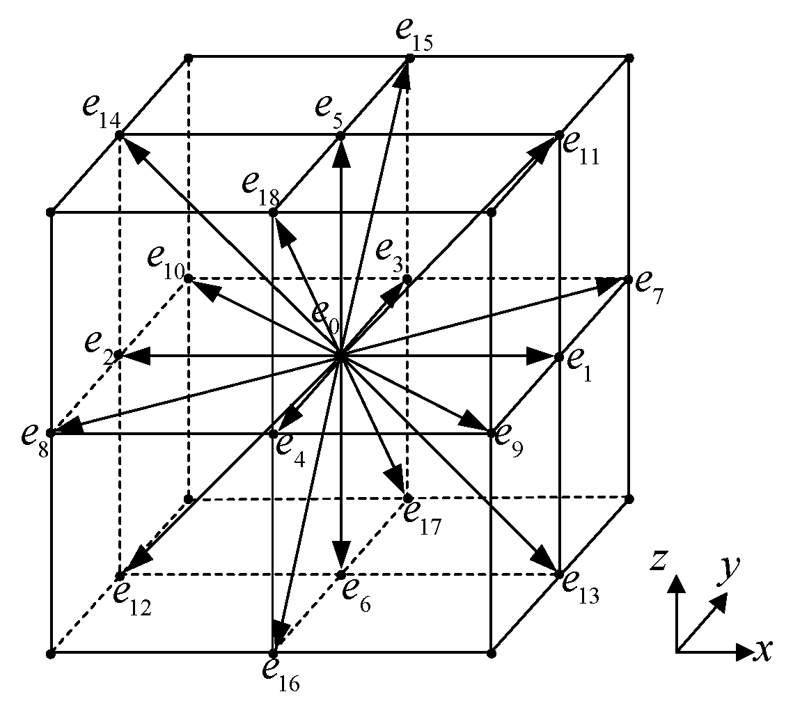
2.1. RLBM-LES

RLBM is an improved model based on LBM. Therefore, RLBM can be derived from the introduction of LBM. LBM deduced from the kinetic theory consists of three parts: a discrete lattice velocity model, equilibrium distribution functions (EDFs), and a time evolution equation [21,46]. The time evolution equation of LBM can be written as:

$$f_i(x+e_{ix}{\delta }_t,y+e_{iy}{\delta }_t,z+e_{iz}{\delta }_t,t+{\delta }_t)-f_i(x,y,z,t)=-\frac{1}{\tau }[f_i(x,y,z,t)-f_i^{eq}(x,y,z,t)],$$

(1)

where $f_i(x,y,z,t)$ is the particle distribution function (PDF) at site $(x,y,z)$ and time t, $f_i^{eq}(x,y,z,t)$ is the equilibrium distribution function at site $(x,y,z)$ and time t, ${\delta }_t$ is the lattice time step, ${\mathit{e}}_i$ is the discrete velocity, and $\tau$ is the dimensionless relaxation time, which is determined by the fluid viscosity $\nu$ of the fluid:

$$\tau =\frac{\nu }{c_s^2}+\frac{\Delta t}{2},$$

(2)

where $c_s$ is the lattice speed of sound, $c_s=\sqrt{3}/3$.

According to the characteristics of LBM, Equation (1) consists of the following parts: collision and streaming,

$$f_i^{+}(x,y,z,t)=f_i(x,y,z,t)+(-\frac{1}{\tau }[f_i(x,y,z,t)-f_i^{eq}(x,y,z,t)]),$$

(3)

$$f_i(x+e_{ix}{\delta }_t,y+e_{iy}{\delta }_t,z+e_{iz}{\delta }_t,t+{\delta }_t)=f_i^{+}(x,y,z,t),$$

(4)

where $f_i^{+}(x,y,z,t)$ denotes the post-collision state of PDF.

When using LBM to simulate three-dimensional fluif flow, the D3Q19 (see Figure 1) model is the most commonly used, and the corresponding discrete velocities ${\mathit{e}}_i$ are:

$$\begin{array}{cc}\hfill \mathit{e}=& c\left(\begin{array}{ccccccccccccccccccc}\hfill 0& \hfill 1& \hfill -1& \hfill 0& \hfill 0& \hfill 0& \hfill 0& \hfill 1& \hfill -1& \hfill 1& \hfill -1& \hfill 1& \hfill -1& \hfill 1& \hfill -1& \hfill 0& \hfill 0& \hfill 0& \hfill 0\\ \hfill 0& \hfill 0& \hfill 0& \hfill 1& \hfill -1& \hfill 0& \hfill 0& \hfill 1& \hfill -1& \hfill -1& \hfill 1& \hfill 0& \hfill 0& \hfill 0& \hfill 0& \hfill 1& \hfill -1& \hfill 1& \hfill -1\\ \hfill 0& \hfill 0& \hfill 0& \hfill 0& \hfill 0& \hfill 1& \hfill -1& \hfill 0& \hfill 0& \hfill 0& \hfill 0& \hfill 1& \hfill -1& \hfill -1& \hfill 1& \hfill 1& \hfill -1& \hfill -1& \hfill 1\end{array}\right),\hfill \end{array}$$

(5)

where the lattice speed $c=\sqrt{3}{c}_s$.

The equilibrium function $f_i^{eq}(x,y,z,t)$ is calculated by the following formula:

$$f_i^{eq}=\rho {\omega }_i\left[1+\frac{{\mathit{e}}_i·\mathit{u}}{c_s^2}+\frac{{({\mathit{e}}_i·\mathit{u})}^2}{2c_s^4}-\frac{{\mathit{u}}^2}{2c_s^2}\right].$$

(6)

In Equation (6), the coefficients of ${\omega }_i$ are ${\omega }_i=1/3$ (${\mathit{e}}_i^2=0$), ${\omega }_i=1/18$ (${\mathit{e}}_i^2=1$) and ${\omega }_i=1/36$ (${\mathit{e}}_i^2=2$). $\rho$ is the fluid density. $\mathit{u}$ is the macroscopic flow velocity.

Latt and Chopard [25] proposed a regularized version of LBM. The main idea of the regularization version is to add an additional regularization step before the collision operation of LBM. The introduction of the regularization step enhances the numerical stability. In the regularized lattice Boltzmann scheme, the non-equilibrium value of the distribution function is defined as:

$$f_i^{neq}=f_i-f_i^{eq}.$$

(7)

Substitute Equation (7) into Equation (1), Equation (1) can be transformed into:

$$f_i(x+e_{ix}{\delta }_t,y+e_{iy}{\delta }_t,z+e_{iz}{\delta }_t,t+{\delta }_t)=(1-\frac{1}{\tau })f_i^{neq}(x,y,z,t)+f_i^{eq}(x,y,z,t).$$

(8)

The non-equlibrium part of the distribution function is related to the first order Chapman-Enskog expansion,

$$f_i^{\mathrm{neq}}\approx f_i^1=-\frac{t_i}{\omega c_s^2}{Q}_{ia\beta }{\partial }_a\rho u_{\beta },$$

(9)

where $Q_{i\alpha \beta }=c_{i\alpha }{c}_{i\beta }-c_s^2{\delta }_{\alpha \beta }$ is a symmetric tensor, which is defined in terms of the Kronecker symbol ${\delta }_{\alpha \beta }$. $t_i$ is the weighting factor of the corresponding grid direction, and the values of $t_i$ are $t_i=1/3$ ($i=0$), $t_i=1/18$ ($i=1\dots 6$) and $t_i=1/36$ ($i=7\dots 18$)

From Chapman-Enskog expansion, the stress tensor ${\prod }_{a\beta }^{neq}={\displaystyle \sum _i^{}}{f}_i^{neq}{c}_{ia}{c}_{i\beta }$ and the velocity gradient has the following relations:

$${\prod }_{\alpha \beta }^{neq}\approx \sum _k^{}{f}_k^1{c}_{k\alpha }{c}_{k\beta }=-\frac{c_s^2}{\omega }({\partial }_{\alpha }\rho u_{\beta }+{\partial }_{\beta }\rho u_{\alpha }).$$

(10)

According to the symmetry of $Q_{i\alpha \beta }=Q_{i\beta \alpha }$, from Equations (9) and (10), we can obtain

$$f_i^1=\frac{t_i}{2c_s^4}{Q}_{ia\beta }{\prod }_{\alpha \beta }^{neq}.$$

(11)

Substituting the above equation into Equation (8), the regularized LBM algorithm can be written as

$$f_i(x+e_{ix}{\delta }_t,y+e_{iy}{\delta }_t,z+e_{iz}{\delta }_t,t+{\delta }_t)=(1-\frac{1}{\tau })f_i^1(x,y,z,t)+f_i^{eq}(x,y,z,t).$$

(12)

The macroscopic density and velocity are given by

$$\begin{array}{c}\rho ={\displaystyle \sum _{i=0}^{18}}{f}_i,\hfill \\ \mathit{u}=\frac{1}{\rho }{\displaystyle \sum _{i=0}^{18}}{f}_i{\mathit{e}}_i.\hfill \end{array}$$

(13)

In order to simulate the turbulent flow with LES, the Smagorinsky sub-grid scale (SGS) model is incorated into the RLBM framwork. According to [47], the relationship between the total viscosity ${\nu }_{total}$ and the total relaxation time ${\tau }_{total}$ can be expressed by the following formula,

$${\nu }_{total}=\nu +{\nu }_t=3({\tau }_{total}-\frac{1}{2}),$$

(14)

where ${\nu }_t$ is an additional viscosity called the turbulent eddy viscosity.

The turbulent eddy viscosity can be expressed as

$${\nu }_t=C_s{\delta }_x^2\left|S_{\alpha \beta }\right|,$$

(15)

where $C_s$ denotes the Smagorinsky constant, ${\delta }_x$ represents the lattice space, and $S_{\alpha \beta }$ ($\alpha ,\beta \in x,y,z$) in Cartesian coordinates is the strain rate tensor, i.e., $S_{\alpha \beta }=({\partial }_{\alpha }{u}_{\beta }+{\partial }_{\beta }{u}_{\alpha })/2$ and $|S_{\alpha \beta }|=\sqrt{2S_{\alpha \beta }{S}_{\alpha \beta }}$. In the RLBM, $S_{\alpha \beta }$ can be computed directly from the non-equilibrium stress tensor ${\prod }_{\alpha \beta }^{\mathrm{neq}}$ and the calculation of $S_{\alpha \beta }$ according to the following formula as in Delbosc et al. [48]:

$$|S_{\alpha \beta }|=\frac{1}{6C_s{\delta }_x^2}(\sqrt{{\nu }^2+18C_s^2{\delta }_x^2\sqrt{{\prod }_{\alpha \beta }{\prod }_{\alpha \beta }}}-\nu ).$$

(16)

Therefore, ${\tau }_{total}$ can be obtained by ${\nu }_{total}$, and  ${\tau }_{total}$ is used to replace the original relaxation time $\tau$ in Equation (12).

2.2. Boundary Condition

2.2.1. Grid-Aligned Botundary

The handling of the boundary condition affects the calculation accuracy, numerical stability and calculation efficiency of RLBM. In this paper, the non-equilibrium extrapolation method developed by Guo et al. [49] is used to deal with the flat boundary. The non-equilibrium extrapolation method has the advantages of reliable numerical stability and second-order accuracy. The non-equilibrium extrapolation scheme can be expressed as:

$$f_i(x_w,y_w,z_w,t)=f_i^{eq}(\rho (x_f,y_f,z_f,t),{\mathit{u}}_w)+[f_i(x_f,y_f,z_f,t)-f_i^{eq}(x_f,y_f,z_f,t)],$$

(17)

where $\rho (x_f,y_f,z_f,t)$ is the density of the adjacent grid point $(x_f,y_f,z_f)$ of the boundary grid point $(x_w,y_w,z_w)$, and ${\mathit{u}}_w$ is the velocity of the boundary grid point $(x_w,y_w,z_w)$.

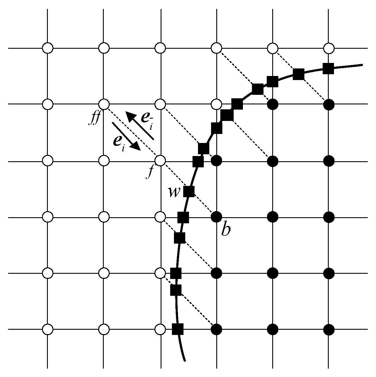
2.2.2. Curved Boundary

The above boundary scheme requires that the grid nodes are on the physical boundary. For more complex curved boundaries, it is difficult for the grid nodes to be exactly on the physical biundary; thus, a new boundary scheme is needed to deal with the curved boundary. In Figure 2, the curved boundary separates the solid nodes from the fluid nodes. The solid circles are the solid nodes and the hollow circles are the fluid nodes. ${\mathit{x}}_f$ is the fluid node near the boundary and ${\mathit{x}}_b$ is the solid node near the boundary. ${\mathit{x}}_{ff}$ is the adjacent fluid node of ${\mathit{x}}_f$. The solid square ${\mathit{x}}_w$ on the curve represents the intersections of the boundary and various lattice links. ${\mathit{u}}_{\mathit{w}}$ is the boundary velocity at point ${\mathit{x}}_w$. The curved boundary scheme can be expressed as follows,

$$f_{\overline{i}}({\mathit{x}}_f,t+{\delta }_t)=\frac{1}{1+q}\left[(1-q)f_i^{+}({\mathit{x}}_{ff},t)+q{f}_i^{+}({\mathit{x}}_f,t)+q{f}_{\overline{i}}^{+}({\mathit{x}}_f,t)\right],$$

(18)

where $\overline{i}$ is the opposite direction of i, and q is the fraction of an intersected link in the fluid region, which is given by:

$$q=\frac{|{\mathit{x}}_f-{\mathit{x}}_w|}{|{\mathit{x}}_f-{\mathit{x}}_b|},0\le q\le 1.$$

(19)

The specific implementation steps of RLBM can be summarized as Figure 3.

3. RLBM Parallel Strategy

According to the execution order of the propagation method, it can be divided into two types, one is to execute the collision step before the propagation step and the other is to execute the propagation step before the collision step [50]. The order of execution in this paper is to use the collision step before the propagation step.

In the RLBM, the execution of the regularization and collision operation is local, and the streaming operation only involves adjacent grid points; thus, the RLBM algorithm is particularly suitable for parallel implementation, and it is a reasonable parallel strategy to divide the flow domain into a sub-domain using the DDM [51]. DDM is a technique in parallel computing; according to the process analysis of RLBM and LES computation, it can be found that under the same scale of the grid, it mainly includes the process of collision, migration, boundary processing, etc., and the process of computation is basically the same at each grid point, so the DDM is used to decompose the whole computational grid area into domains in accordance with the principle of computational load balancing.

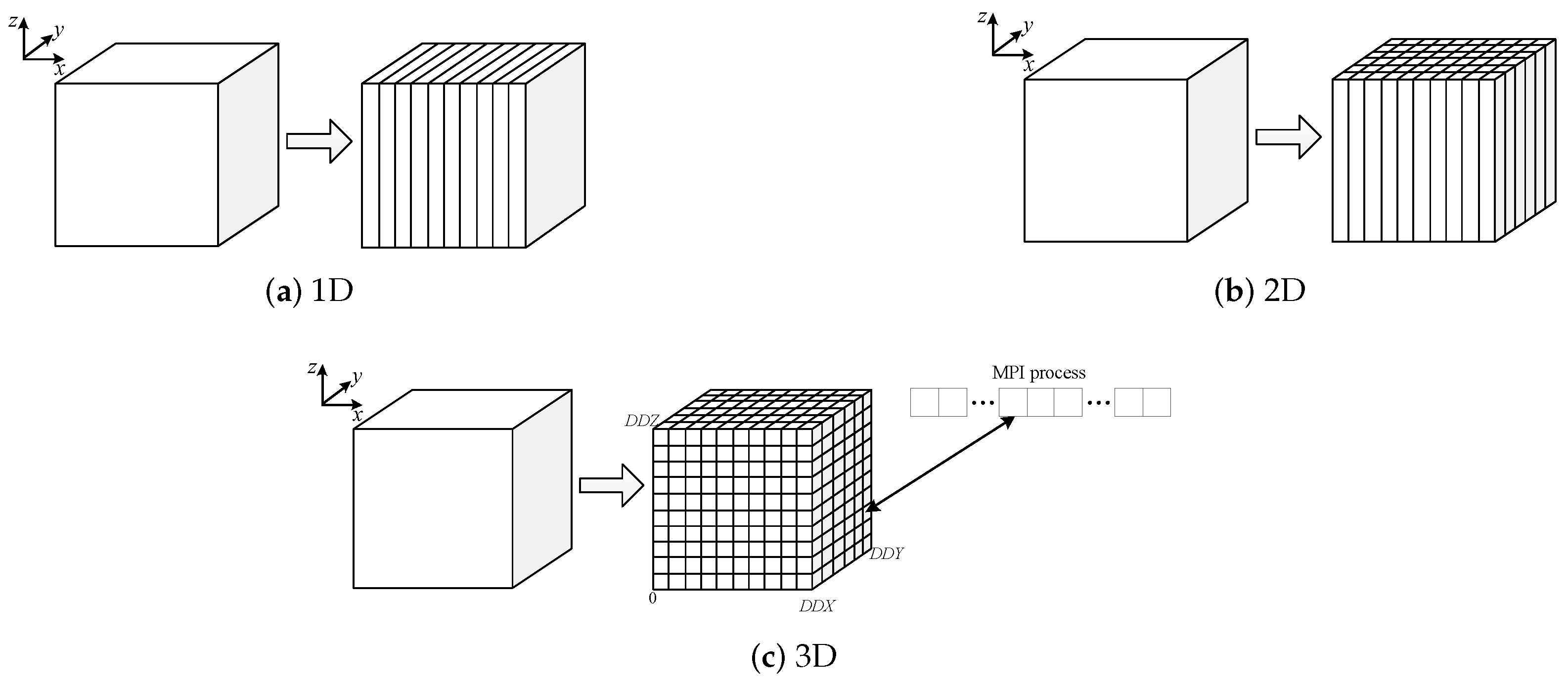
3.1. Domain Decomposition

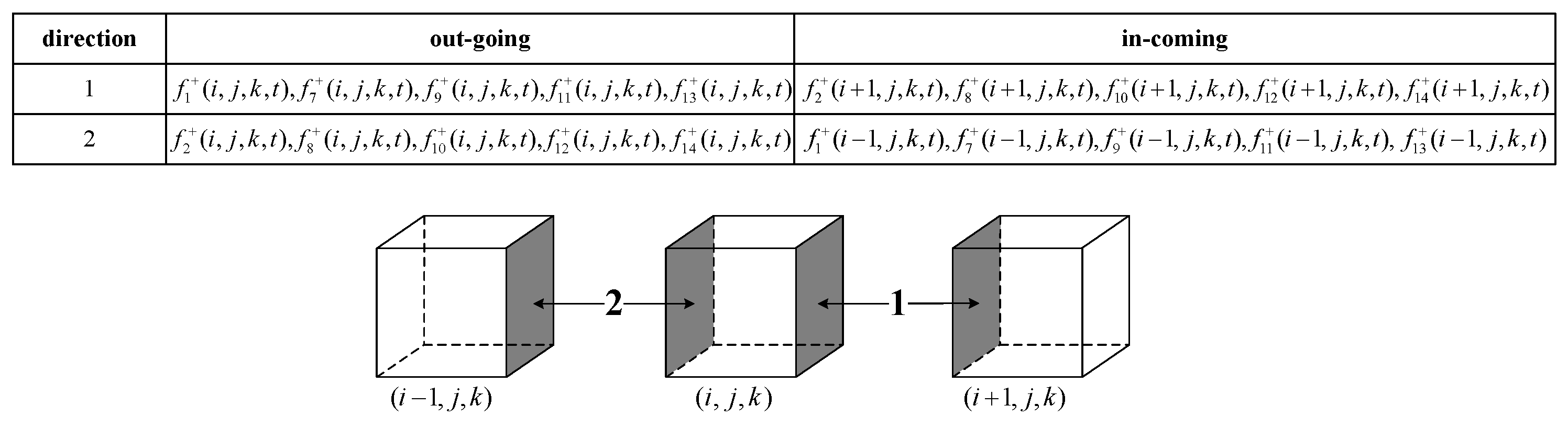
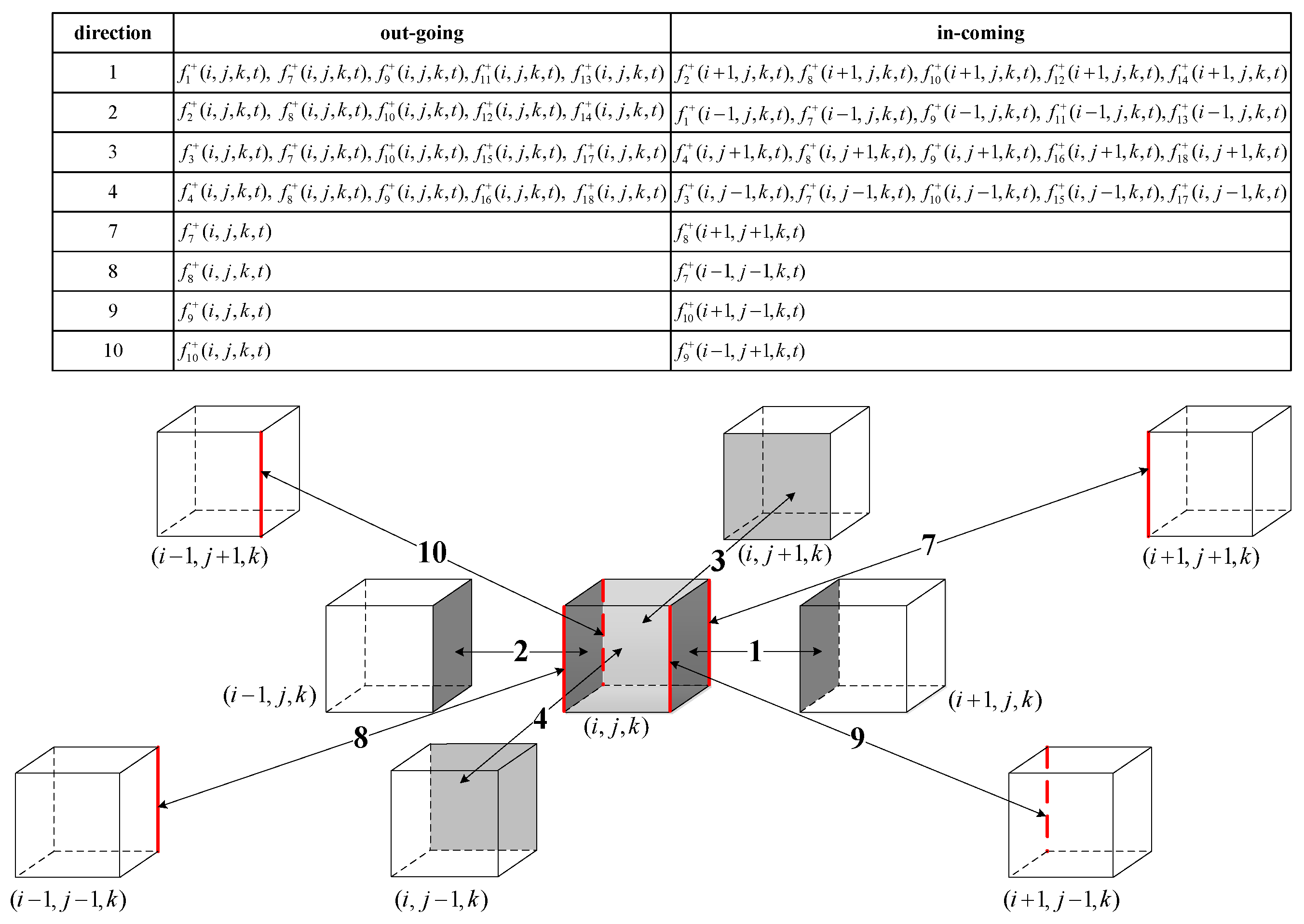
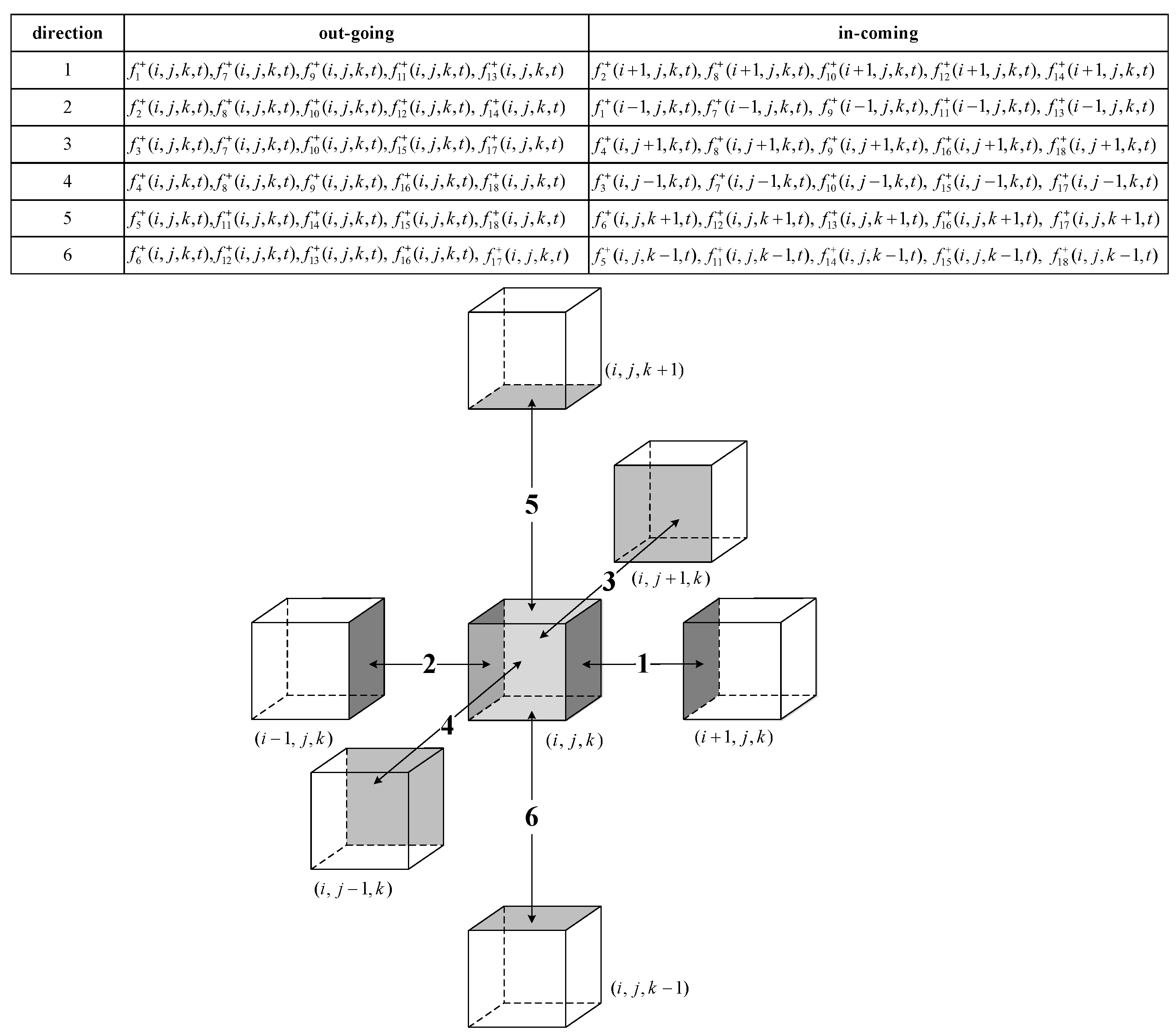
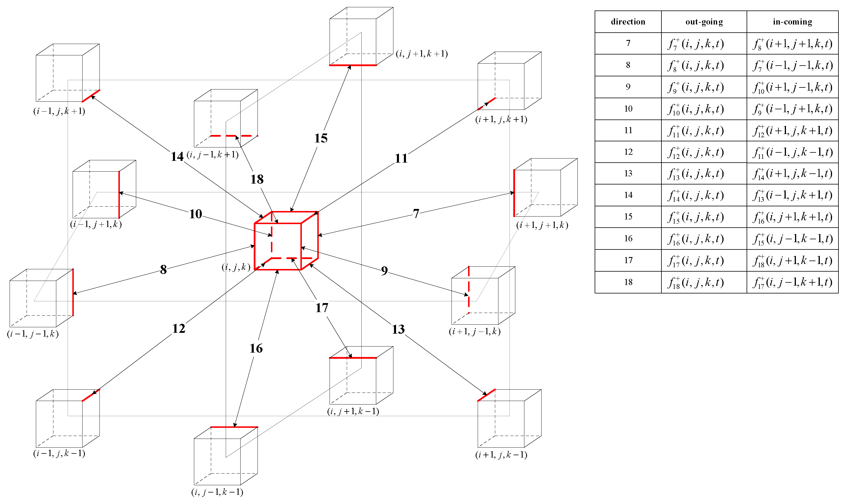
For the three-dimensional case, the domain decomposition can be decomposed in one direction (1D) (see Figure 4a), two directions (2D) (see Figure 4b) or three directions (3D) (see Figure 4c).

As shown in Figure 4c, after domain decomposition, each sub-domain corresponds to an MPI process. Because the process is one-dimensional, the dimension of domain decomposition may be one-dimensional, two-dimensional or three-dimensional. Therefore, a connection needs to be established between them. Taking the three-dimensional subdomain $(i,j,k)$ as an example, the relationship is as follows:

$$\left.\begin{array}{cc}\hfill i& =mod\left(mod\right(prank,nDDX\times nDDY),nDDX)\hfill \\ \hfill j& =\frac{mod(prank,nDDX\times nDDY)}{nDDX}\hfill \\ \hfill k& =\frac{prank}{nDDX\times nDDY}\hfill \end{array}\right\}.$$

(20)

where $nDDX$, $nDDY$, and $nDDZ$ represent the number of domain decompositions along the directions of x, y and z, respectively, and $prank$ is the MPI process rank. Then, the size of the sub-domain in the x direction can be calculated as follows:

$$XBeg=i\times \frac{nLatX}{nDDX}+minInt(i,mod(nLatX,nDDX)),$$

(21)

$$XEnd=\left\{\begin{array}{cc}XBeg+\frac{nLatX}{nDDX}-1\hfill & \hfill mod(nLatX,nDDX)\le i\\ XBeg+\frac{nLatX}{nDDX}\hfill & \hfill mod(nLatX,nDDX)>i\end{array},\right.$$

(22)

where $nLatX$ represents the number of lattice nodes in the x direction. $XBeg$ and $XEnd$ are the begin and end points of the lattice node of sub-domain along x direction, respectively. Similarly, the sub-domain range in the direction of y and z.

When two of $nDDX$, $nDDY$, and $nDDZ$ are set to 1, that is 1D, and one is set to 1, that is 2D.

3.2. Data Exchange

In order to ensure that the calculation results of each sub-domain are accurate, a data exchange with adjacent MPI processes is required. When data are exchanged, it is not necessary to exchange possessive data $f_i^{+}$ in all 18 directions; it is only needed to exchange the $f_i^{+}$ in the directions required for the streaming operation.

In this work, buffers are introduced in order to reduce the complexity of the parallel algorithm design and the ease of program implementation. A buffer is a unit with a data storage function that ensures that the computation is essentially the same at each grid point in each process. At the same time, the increased buffer does not need to participate in the computation and is only used for data storage in the parallel data exchange process. This enables the reduction of the complexity of the algorithm implementation without increasing the amount of computations. According to DDM, these received data are stored in the buffer in the sub-domain, and the size of the buffer depends on DDM.

Figure 5 shows the data exchange of 1D domain decomposition. The sub-domain $(i,j,k)$ exchange data with the adjacent sub-domain that includes four surfaces. The $f_i^{+}$ exchanged in each direction are shown in the table in Figure 5.

Figure 6 shows the data exchange of the 2D domain decomposition. In Figure 6, the sub-domain $(i,j,k)$ exchange data with the adjacent sub-domain, including eight surfaces of data and eight edges of data. The $f_i^{+}$ exchanged in each direction are shown in the table in Figure 6.

Figure 7 and Figure 8 show the data exchange of 3D domain decomposition. In Figure 7, the sub-domain $(i,j,k)$ exchanges 12 surfaces of data with the adjacent sub-domain. In Figure 8, the sub-domain $(i,j,k)$ exchanges 24 edges of data with the adjacent sub-domain The $f_i^{+}$ exchanged in each direction are shown in the table in Figure 7 and Figure 8.

In 1D domain decomposition along the x direction, communication data count is

$$4surfaces=4\times 5\times nLatY\times nLatZ=20\times nLatY\times nLatZ,$$

(23)

where $nLatY$ and $nLatZ$ are the number of lattice nodes along the y and z direction, respectively.

In 2D domain decomposition along the x and y direction, the communication data count is

$$\begin{array}{cc}\hfill 8surfaces + 8edges& = 4 \times 5 \times \frac{nLatX}{nDDX} \times nLatZ + 4 \times 5 \times \frac{nLatY}{nDDY} \times nLatZ\hfill \\ & +8 \times nLatZ\hfill \\ \hfill & =20 \times \frac{nLatX}{nDDX} \times nLatZ + 20 \times \frac{nLatY}{nDDY} \times nLatZ\hfill \\ & +8 \times nLatZ,\hfill \end{array}$$

(24)

In 3D domain decomposition along the x, y and z direction, the communication data count is

$$\begin{array}{cc}\hfill 12surfaces+24edges& =4 \times 5 \times \frac{nLatX}{nDDX} \times \frac{nLatY}{nDDY}+4 \times 5 \times \frac{nLatY}{nDDY} \times \frac{nLatZ}{nDDZ}\hfill \\ & +4 \times 5 \times \frac{nLatX}{nDDX} \times \frac{nLatZ}{nDDZ}+8 \times \frac{nLatX}{nDDX}\hfill \\ & +8 \times \frac{nLatY}{nDDY}+8 \times \frac{nLatZ}{nDDZ}\hfill \\ \hfill & =20 \times \frac{nLatX}{nDDX} \times \frac{nLatY}{nDDY}+20 \times \frac{nLatY}{nDDY} \times \frac{nLatZ}{nDDZ}\hfill \\ & +20 \times \frac{nLatX}{nDDX} \times \frac{nLatZ}{nDDZ}+8 \times \frac{nLatX}{nDDX}+8 \times \frac{nLatY}{nDDY}\hfill \\ & +8 \times \frac{nLatZ}{nDDZ}.\hfill \end{array}$$

(25)

As is observed from

Table 1. Communication data amount among three kinds of DDMs.

DDM	nDDX	nDDY	nDDZ	$\frac{\mathit{nLatX}}{\mathit{nDDX}}$	$\frac{\mathit{nLatY}}{\mathit{nDDY}}$	$\frac{\mathit{nLatZ}}{\mathit{nDDZ}}$	Communication Amount
1D	(0, $nLatX$)	1	1	(0, $nLatX$)	512	512	5,242,880
2D	256	8	1	2	64	512	679,936
	128	16	1	4	32	512	372,736
	64	32	1	8	16	512	249,856
3D	256	4	2	2	128	256	673,808
	128	8	2	4	64	256	355,872
	128	4	4	4	128	128	350,240
	64	16	2	8	32	256	212,288
	64	8	4	8	64	128	196,160
	32	32	2	16	16	256	171,264
	32	16	4	16	32	128	134,528
	32	8	8	16	64	64	124,032
	16	16	8	32	32	64	103,424

, various DDMs are compared according to the lattice scale $512 \times 512 \times 512$.

From Table 1, it can be noted that the 1D domain decomposition does not change the communication data count. When $\frac{nLatX}{nDDX}$, $\frac{nLatY}{nDDY}$, $\frac{nLatZ}{nDDZ}$ gradually becomes equal, the 3D DDM has less communication data count than the 2D one, and the 2D DDM has less communication data count than the 1D one. Thus, the 3D DDM should have better scalability than the 2D one, and the 2D DDM has better scalability than the 1D one.

3.3. Generate the Cartesian Grid

According to the domain decomposition, each sub-domain can judge their lattice type based on the read surface mesh file of geometry, respectively, and there is no need to communicate with other MPI processes. The parallel algorithm of Cartesian grid generation is shown in Algorithm 1.

Algorithm 1 Parallel algorithm of Cartesian grid generation.

1: Obtain the lattice count (noted as $latticeCount$) of the sub-domain based on Equations (21) and (22); 2: Each MPI process generates the initial Cartesian grid, repectively; 3: Judge the lattice type; 4: For (int $i=0$; i < $latticeCount$; i++) 5:      Product type (type[i]) of all lattice in each MPI process according to the relationship between          point and geometry; 6:      if(type[i] == ’boundary’) 7:           Compute the distance between curved boundary lattice and boundary wall [52] and obtain q by               Equation (19);

As is shown in Algorithm 1, each MPI process has to determine each lattice type in the buffer which has an effect on the parallel efficiency of Cartesian grid generation. The amount of Cartesian grid of three kinds of domain decomposition needed to be judged in each MPI process and can be described as follows:

$$A_{1D}=\left(\frac{nLatX}{nDDX}+2\right)\times nLatY\times nLatZ,$$

(26)

$$A_{2D}=\left(\frac{nLatX}{nDDX}+2\right)\times \left(\frac{nLatY}{nDDY}+2\right)\times nLatZ,$$

(27)

$$A_{3D}=\left(\frac{nLatX}{nDDX}+2\right)\times \left(\frac{nLatY}{nDDY}+2\right)\times \left(\frac{nLatZ}{nDDZ}+2\right),$$

(28)

where $A_{1D}$, $A_{2D}$, and $A_{3D}$ denote the amount of lattice needed to judge the lattice type in 1D, 2D, and 3D DDM, respectively. It can be observed from

Table 2. Comparison of lattice needed to be judged among three kinds of domain decomposition.

DDM	nDDX	nDDY	nDDZ	$\frac{\mathit{nLatX}}{\mathit{nDDX}}$	$\frac{\mathit{nLatY}}{\mathit{nDDY}}$	$\frac{\mathit{nLatZ}}{\mathit{nDDZ}}$	Lattice Amount
1D	2048	1	1	1	512	512	786,432
2D	256	8	1	8	64	512	337,920
	128	16	1	16	32	512	313,344
	64	32	1	32	16	512	313,344
3D	256	4	2	8	128	256	335,400
	128	8	2	16	64	256	306,504
	128	4	4	16	128	128	304,200
	64	16	2	32	32	256	298,248
	64	8	4	32	64	128	291,720
	32	32	2	64	16	256	306,504
	32	16	4	64	32	128	291,720
	32	8	8	64	64	64	287,496
	16	16	8	128	32	64	291,720

that $A_{1D}$, $A_{2D}$, and $A_{3D}$ are compared based on the lattice scale $2048\times 512\times 512$. Different DDMs have similar computational complexities; the difference depends on the buffers of different domain decomposition. When $\frac{nLatX}{nDDX}$, $\frac{nLatY}{nDDY}$, $\frac{nLatZ}{nDDZ}$ gradually become equal, 3D DDM has least amount of lattice needed to be judged.

3.4. RLBM Parallel Algorithm

RLBM parallel iterative calculation can be described as an Algorithm 2. We first read the surface mesh file, then the domain decomposition and the calculation of sub-domain range are carried out. After generating a Cartesian grid, the flow field information is initialized, and then the RLBM parallel iterative calculation starts. The regularization calculation is required before the collision. After the collision, the MPI process must exchange data with the neighboring processes based on DDM. After the data exchange, the propagation operation is carried out, and finally the boundary and macro-quantity calculations are carried out. Compared to the serial RLBM algorithm shown in Figure 3, the parallel RLBM Algorithm 2 includes the domain decomposition method, Cartesian grid generation and MPI communication.

According to the computational features of the combination of RLBM and LES, since RLBM involves only the information of local neighboring nodes in the process of computation, it adopts the computational volume load priority (i.e., the computational volume corresponding to the mesh division is basically the same), and then designs the communication strategy based on it to realize the load balancing based on MPI. Parallel algorithms need to be designed with adaptability on high performance computers in mind. Since high performance computers have a departmental structure with distributed storage, MPI techniques must be used to implement the data exchange.

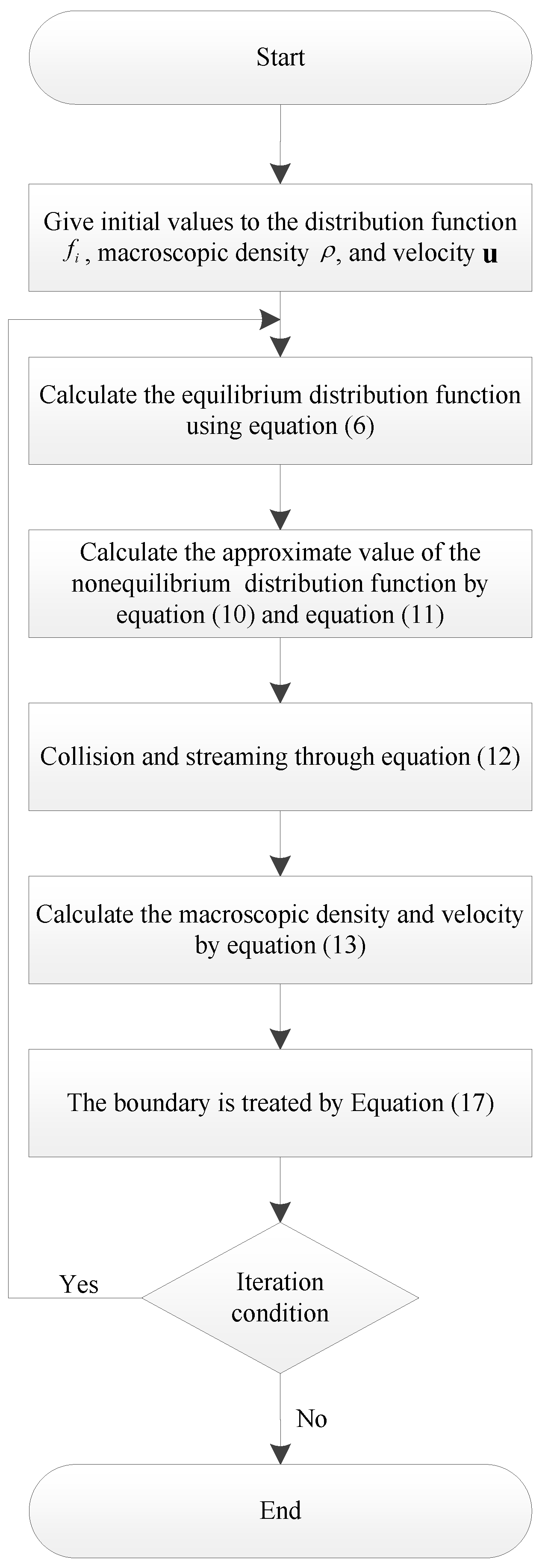
Algorithm 2 RLBM Parallel Iterative Computation.

1: Read the STL file to generate a calculation model; 2: Select the appropriate dimension to decompose the domain and compute the range of sub-domain; 3: Generate the Cartesian grid; 4: Initial flow field informance; 5: RLBM parallel iterative computation until satisfying the convergence condition:     (a) Regularization calculation through Equation (11);     (b) Collision through Equation (12);     (c) Exchange data with neighbor MPI processes;     (d) Streaming through Equation (12);     (e) Deal with boundary conditions;     (f) Calculate the macroscopic density $\rho$ and velocity $\mathit{u}$ based by Equation (13).

4. Numerical Experiment

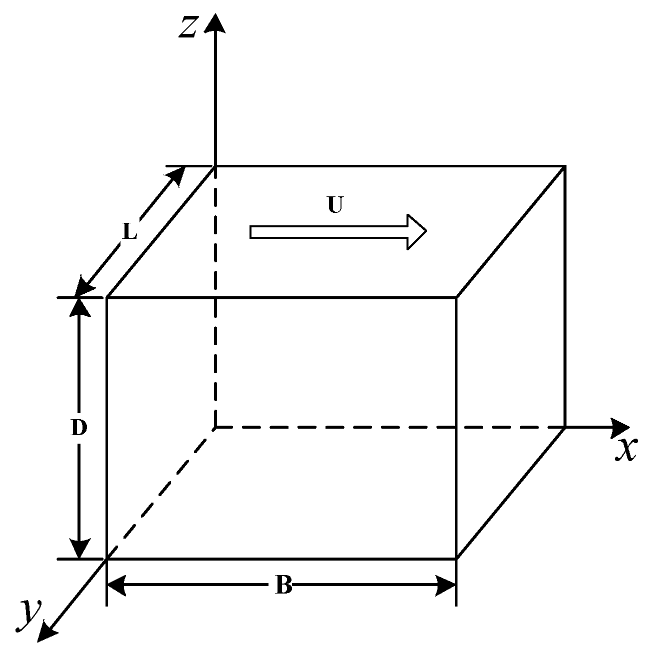
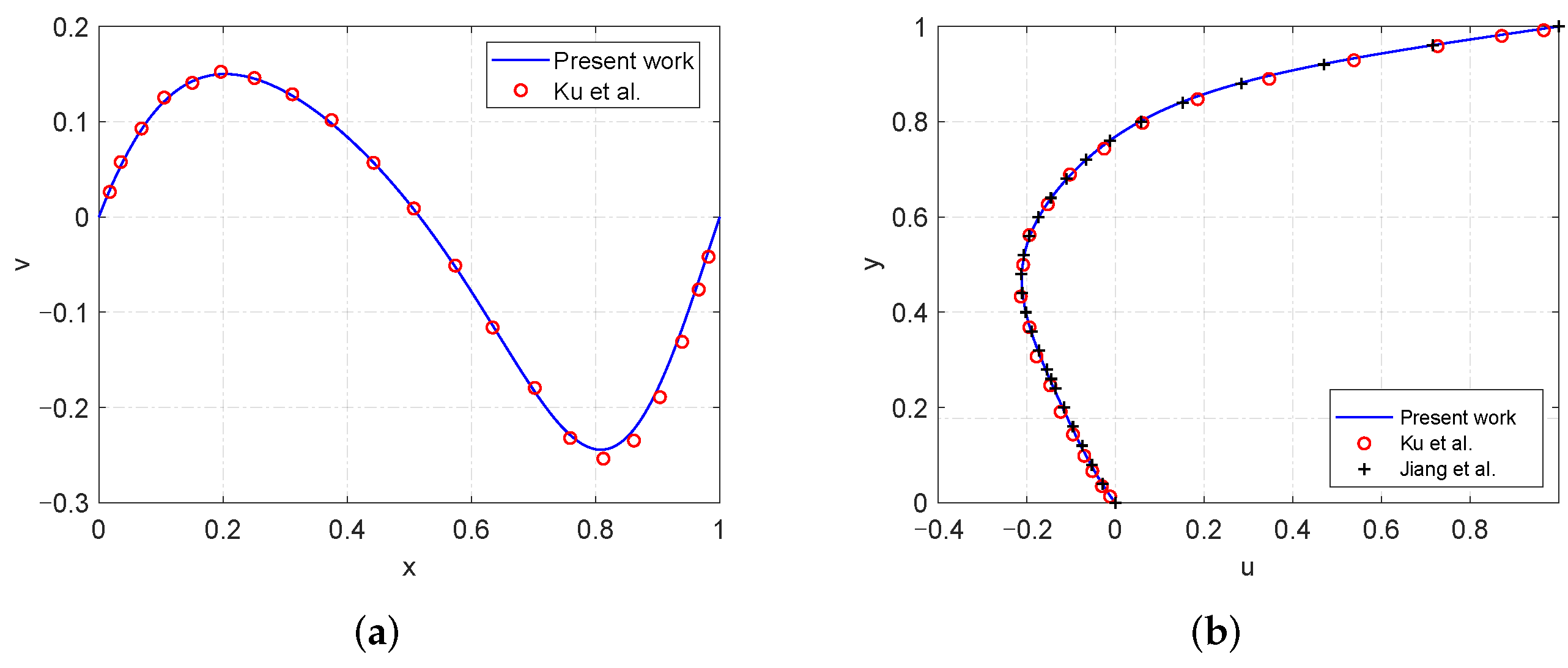
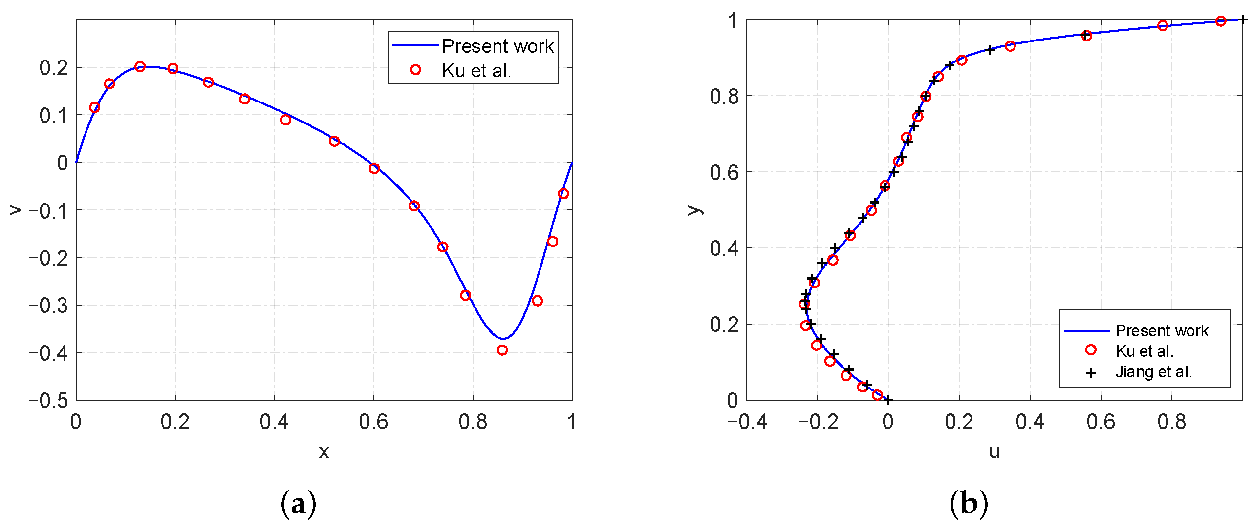
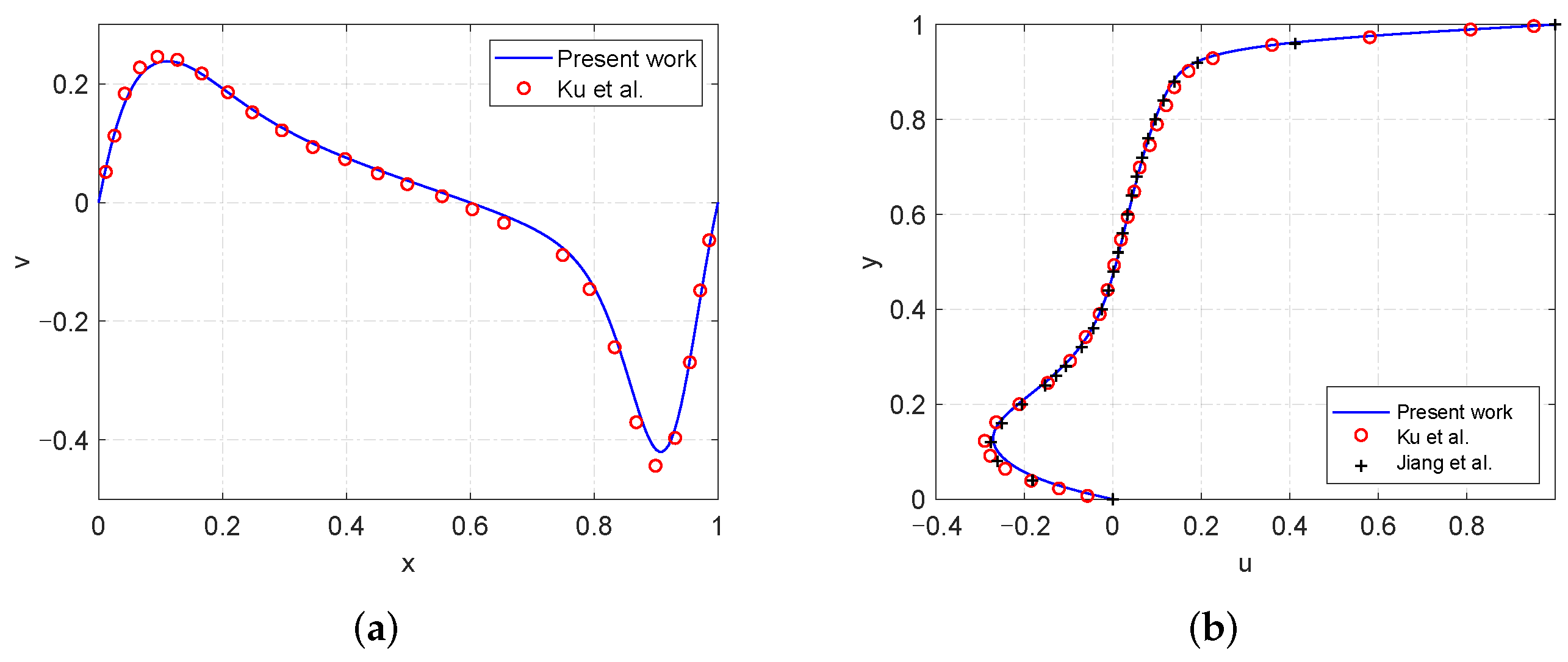
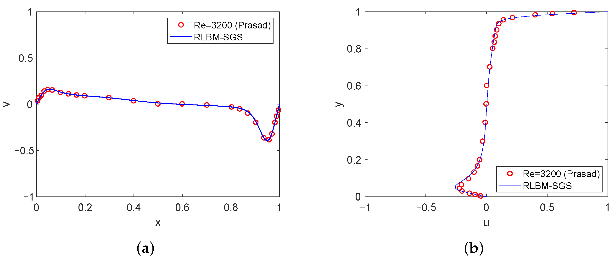
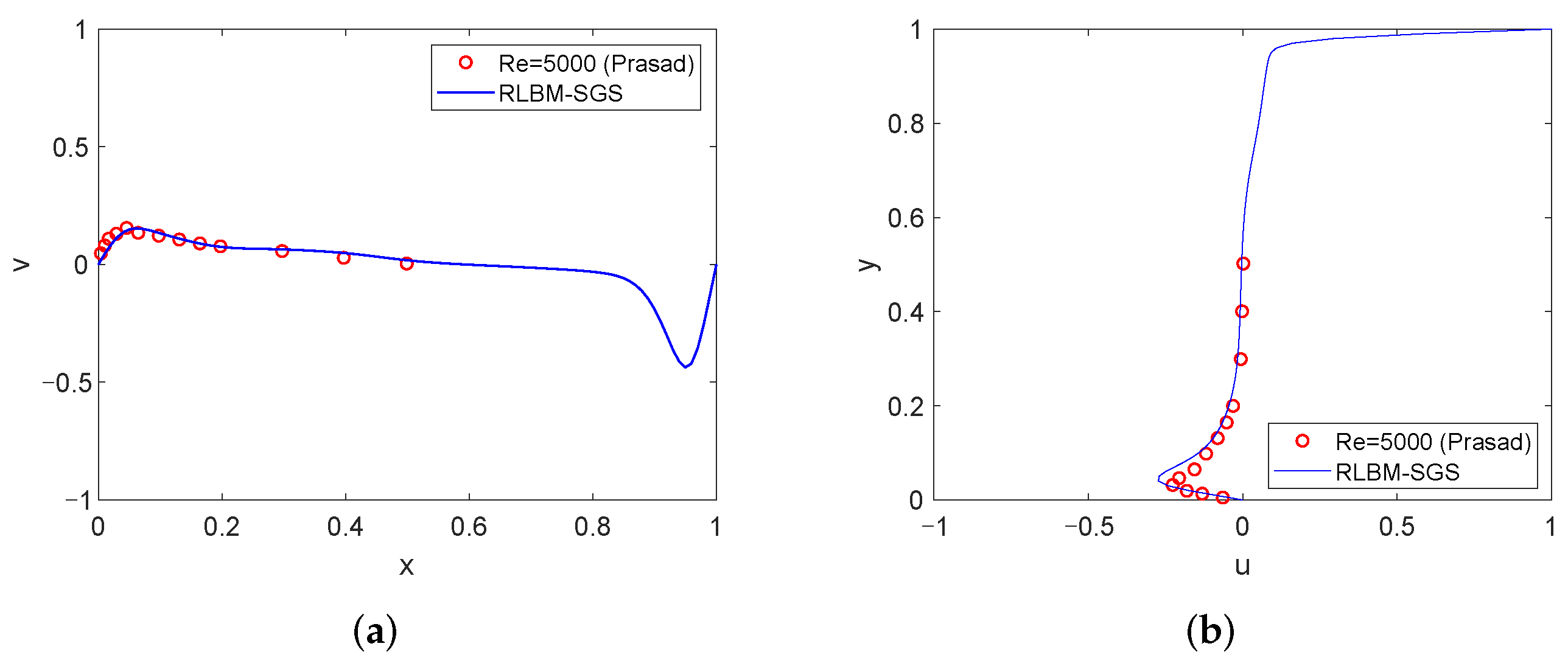
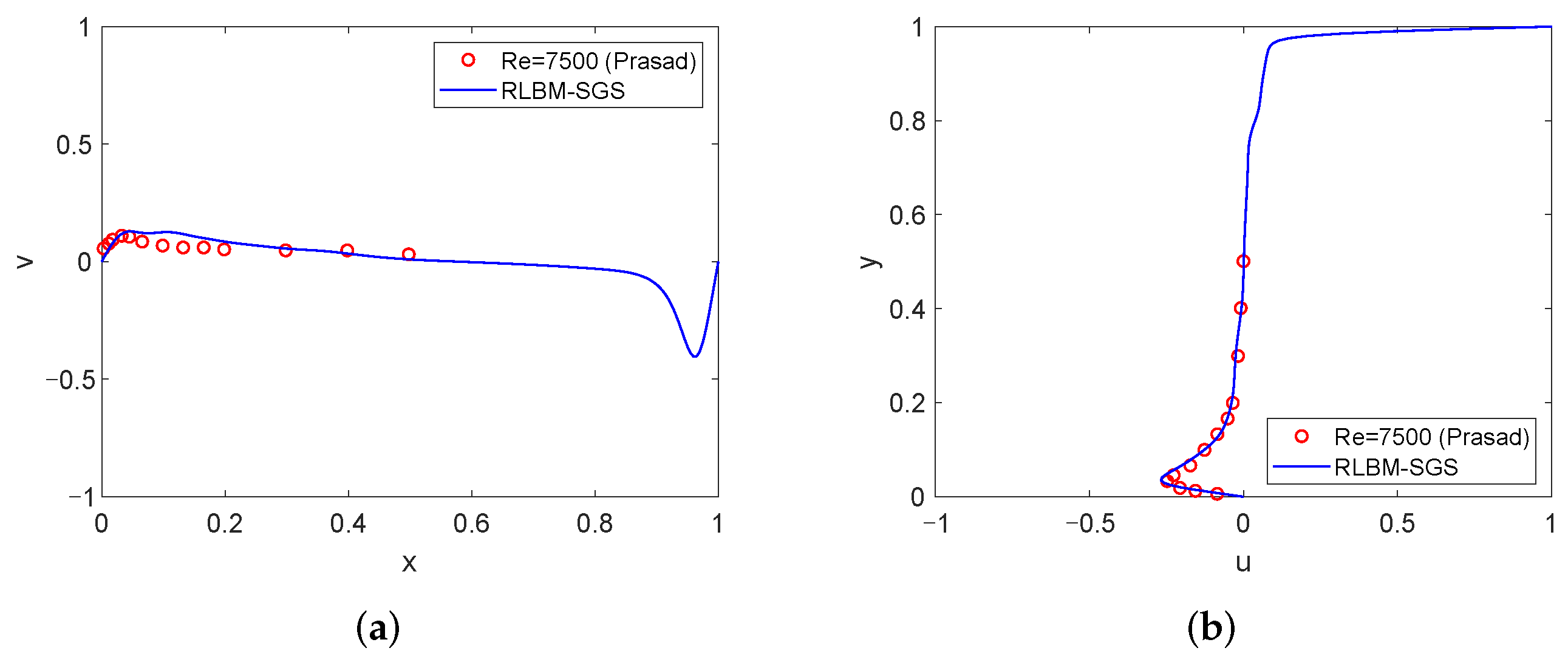
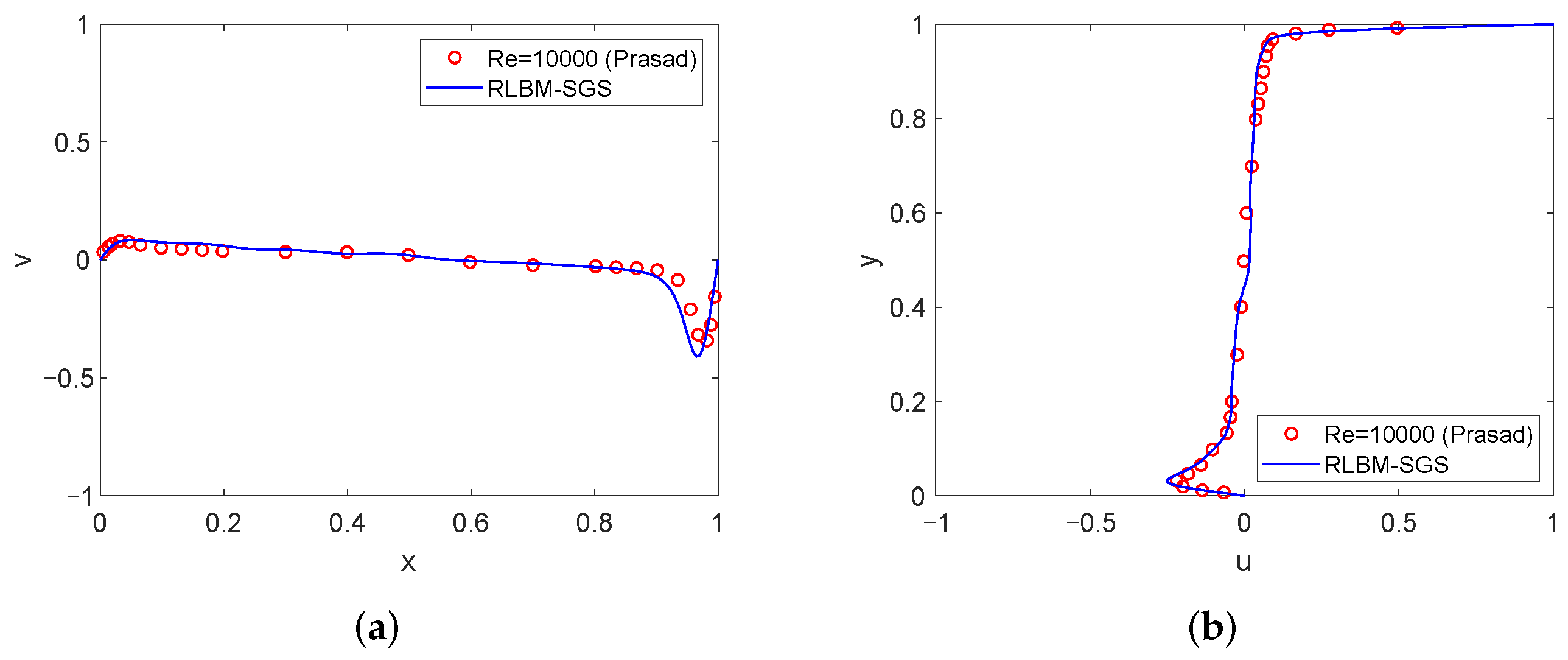
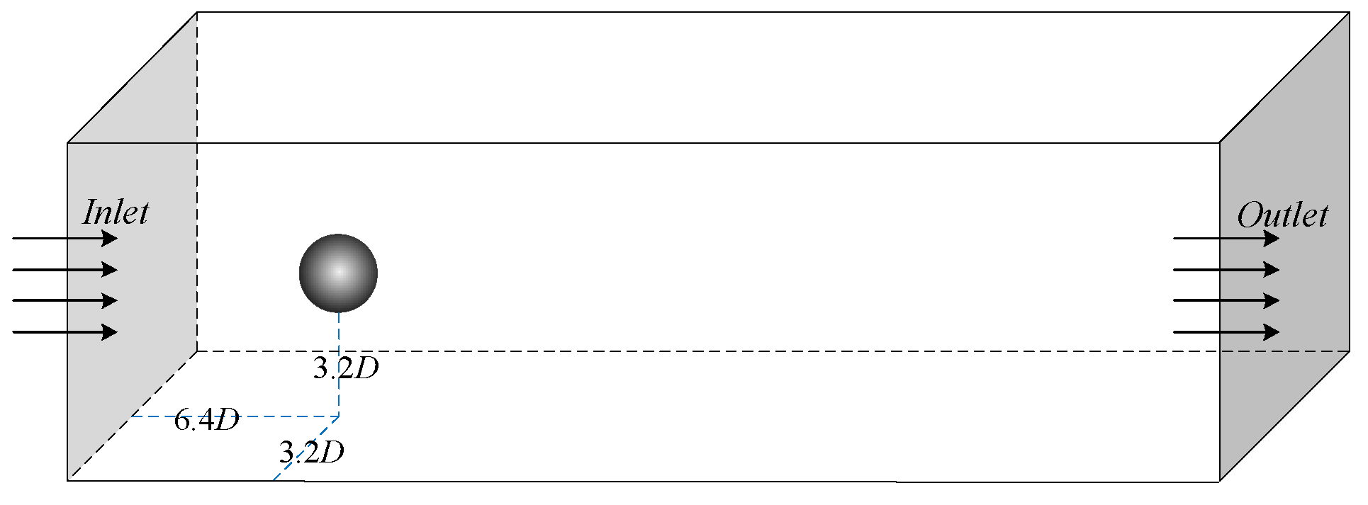
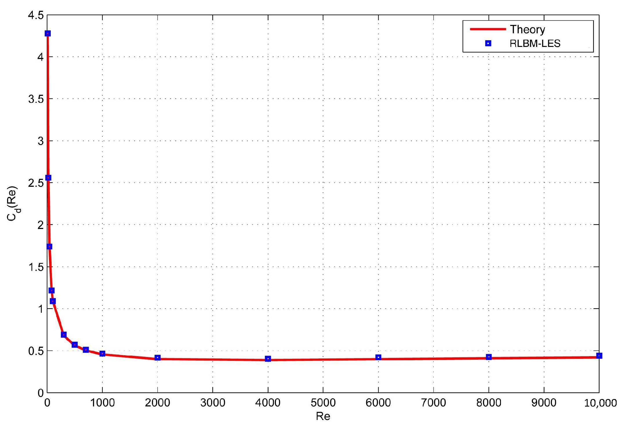
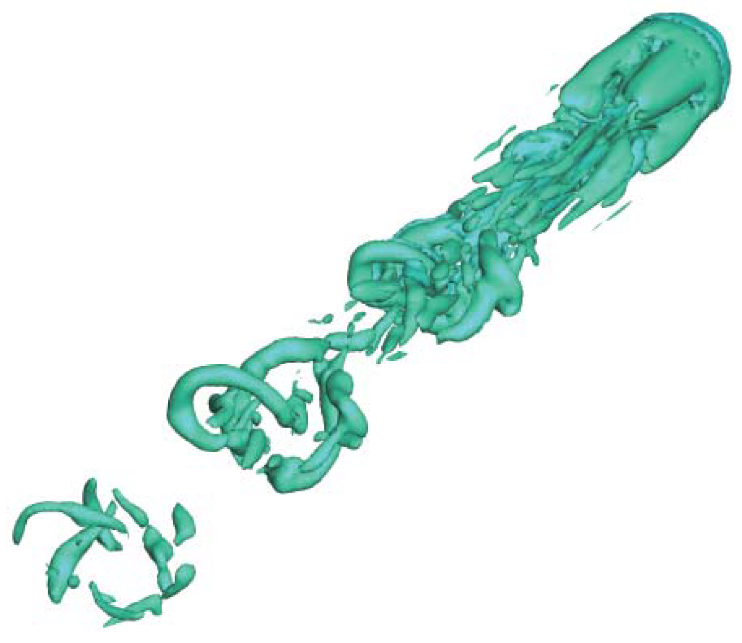
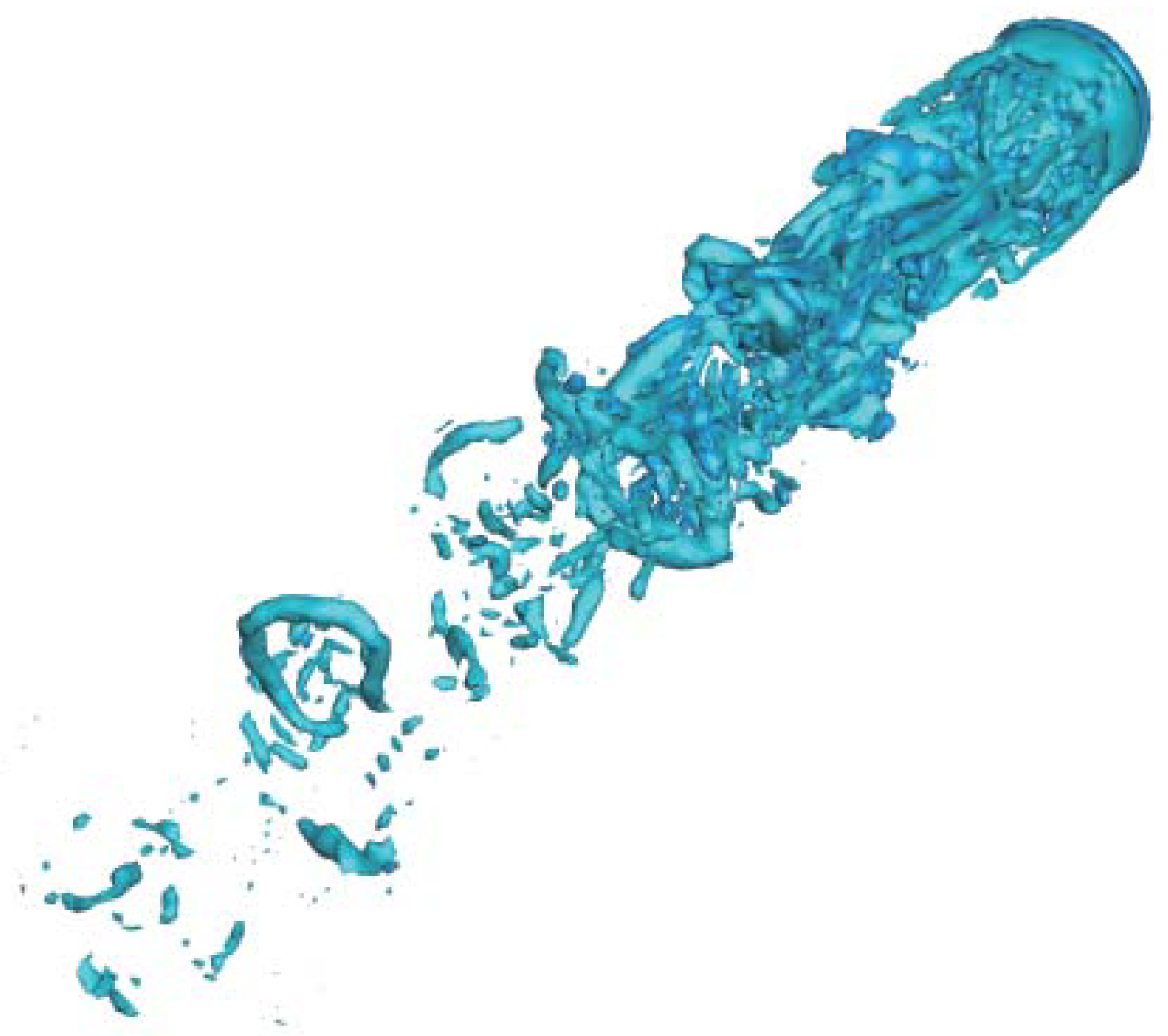
4.1. High Reynolds Number Simulation

In this section, a 3D lid-driven cavity flow with a constant lid velocity $\mathrm{U}$ was simulated as a numerical test for our experiments.The 3D lid-driven cavity flow is a regularly shaped computational region, which can be used as a benchmark for verifying a parallel algorithm in terms of acceleration ratio and parallel efficiency. Therefore, the 3D lid-driven cavity flow is used in this paper, through which the results of the parallel algorithm designed in this paper are proved to be accurate. On this basis, it is further verified that the parallel algorithm designed in this paper also has good parallel speedup and parallel efficiency. In terms of units, for the sake of ease in experimental programming, we conducted a dimensionless analysis on all physical quantities and ensured that the dimensionless flow and heat transfer criteria remained consistent before and after the nondimensionalization process. Figure 9 shows the geometry of the lid-driven cavity flow. In Figure 9, $\mathrm{B}$ is the cavity width, $\mathrm{D}$ is the cavity height, $\mathrm{L}$ is the cavity length, and $\mathrm{U}$ is a constant lid velocity. In the experiments of this paper, the spanwise aspect ratio ($\mathrm{SAR}=\mathrm{L}/\mathrm{B}$) is 0.5:1 or 1:1, and the depthwise aspect ratio ($\mathrm{DAR}=\mathrm{D}/\mathrm{B}$) is fixed at 1:1.

The RLBM algorithm using MPI is used to simulate the 3D lid-driven cavity flow with different Reynolds numbers. We prove the accuracy of the algorithm by simulating the Reynolds number of 100, 400, and 1000. Figure 10, Figure 11 and Figure 12 show a comparison of the RLBM results of the lid-driven cavity flow with the results of Ku et al. [53] and Jiang et al. [54]. It can be found that the RLBM algorithm using MPI in this paper is accurate.

Then, we added Sub-Grid Scale(SGS) to the RLBM algorithm using MPI to simulate the 3D lid-driven cavity flow with a high Reynolds number. Figure 13, Figure 14, Figure 15 and Figure 16 show the comparision between the results of the RLBM-SGS algorithm using MPI under the high Reynolds number and the results of Prasad et al. [55]. It can be found that the RLBM-SGS has a good stability under the high Reynolds number.

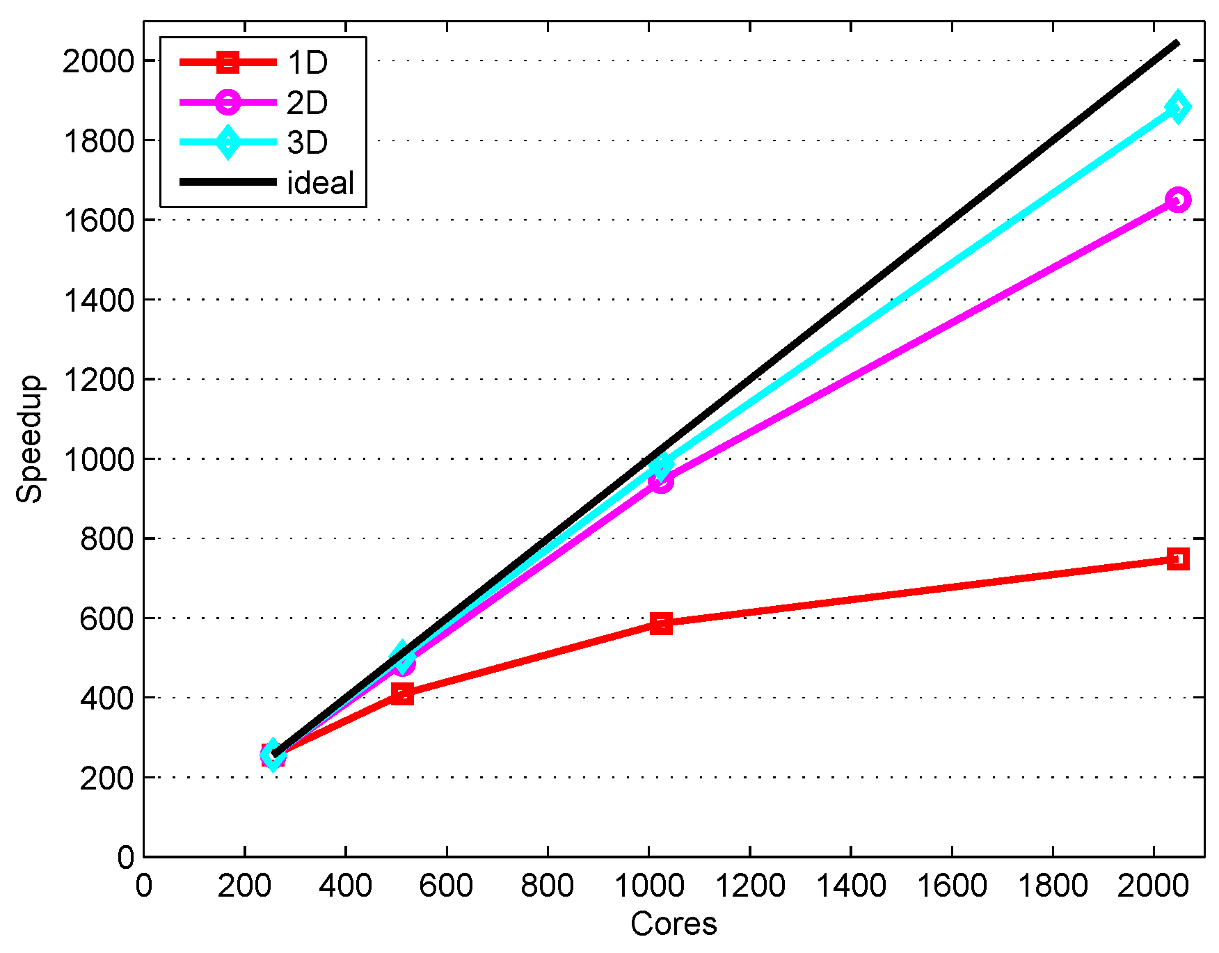
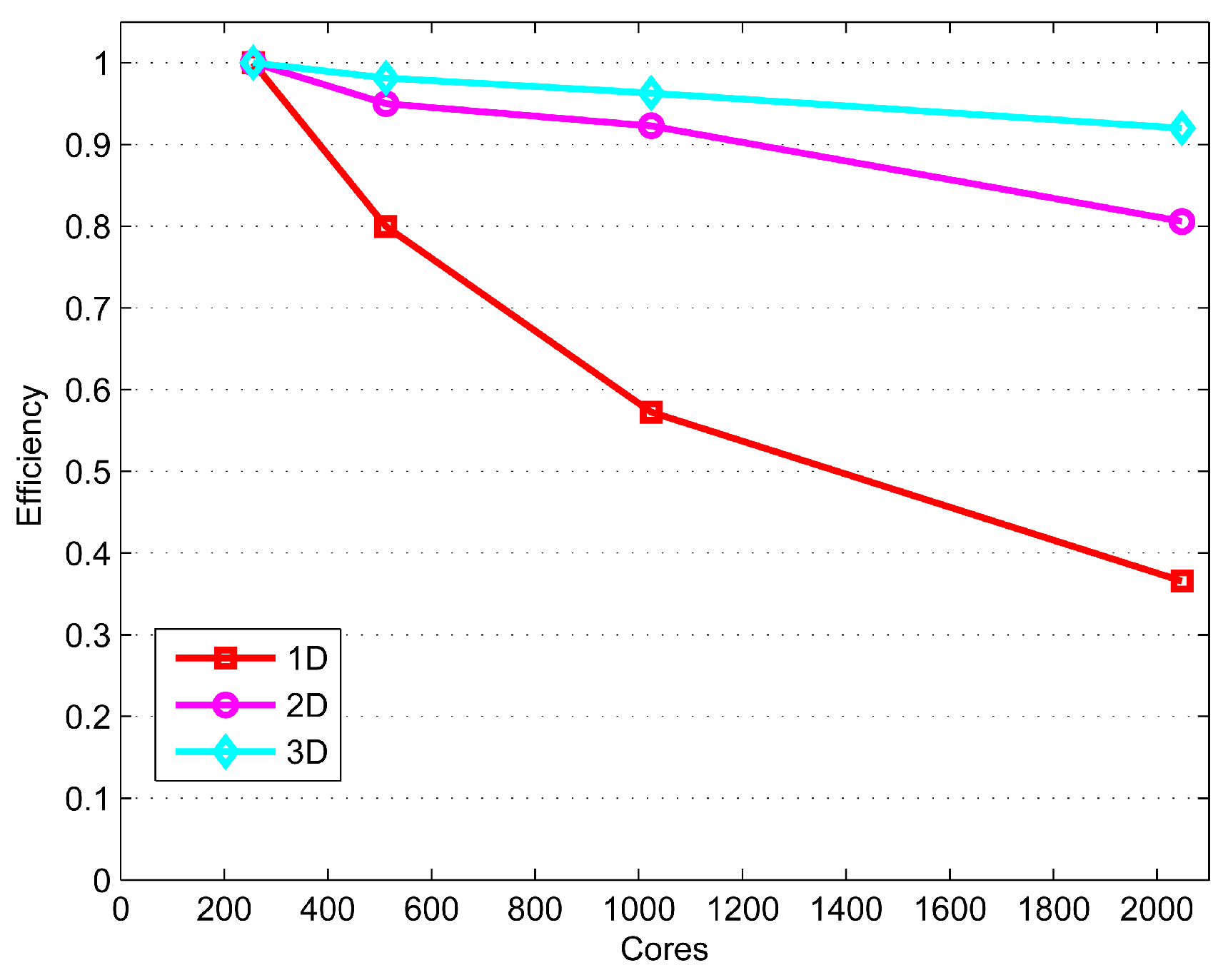
4.2. Comparison of Three Kinds of Domain Decomposition Methods

In this section, a 3D incompressible flow around a sphere with a constant velocity profile, $u=U_{\infty }=\{0.2Ma,0,0\}$, was simulated as a numerical test for our various domain decomposition methods. Figure 17 shows the schematic diagram of a three-dimensional flow past a circular cylinder. In order to eliminate the influence of the boundary, the three-dimensional (length × width × height) size of the calculation domain is $51.2D$, $12.8D$ and $12.8D$, respectively. D is the radius of the sphere, and its value is 40. The grid scale is 2048 × 512 × 512.

This comparison experiment was carried out on the third-generation cluster high-performance computer-“Ziqiang 4000” of Shanghai University. The cluster includes 140 CPU compute nodes. Each node has two Intel SandyBridge architecture CPUs (Intel E5-2690, 2.9 GHz/8-core), and the cluster has a total of 2240 cores. The shared running memory of each node is 64 GB. The code is compiled under the mpich2 and GCC compilation environment, and the optimization level of the code is “-O3”.

The drag force on the sphere $F_d$ is computed with the momentum-exchange method [56], and the drag force coefficient [57] is obtained by

$$C_d=-\frac{8F_d}{\rho u_{\infty }^2{D}^2}.$$

(29)

The Figure 18 shows that our experiments are in good agreement with theoretical value [58]. Figure 19 and Figure 20 describe the vortical structure when Re = 1000 and 3700, respectively.

In

Table 3. Computational time among three kinds of domain decomposition.

	nPX	nPY	nPZ	Iterative Time (s)	Communication Time (s)	Time to Generate Grid (s)
1D	256	1	1	1410.78	53.2321	13.9915
	512	1	1	882.0	54.5075	9.30438
	1024	1	1	616.1	53.7755	6.59018
	2048	1	1	482.4	54.7407	5.28579
2D	32	8	1	1172.85	12.9407	14.0736
	64	8	1	624.2	10.3737	10.2649
	64	16	1	321.2	7.70774	6.99043
	128	16	1	183.9	6.26043	5.32507
3D	16	4	4	1152.59	10.3427	9.4711
	32	4	4	592.6	7.17983	8.72643
	16	8	8	301.9	4.81678	5.17024
	64	8	4	157.9	3.48762	8.16628

, the time with 100 iterations to generate the grid; communication time and iterative time, including collision time, streaming time, and communication time; are presented.

In 1D DDM, the amount of data needed to be transferred is fixed in accord with Equation (23); thus, the communication time is about same. Using 2D or 3D DDM, the communication time decreases with the increase in $nPX$, $nPY$ or $nPZ$, and the communication time is less under the same cores when adopting the 3D one.

The lattice scales are the same in different DDM; thus, the time to generate the grid is relative when cores are same. The values among three kinds of DDMs show that the iterative time of the 3D one is shorter than the 2D one, and the 2D one has a shorter iterative time than the 1D one. Based on the values of Table 3, speedup and efficiency are shown in Figure 21 and Figure 22. It can be observed that 3D DDM has the best scalability among the three divisions.The 3D DDM also has less communication in the design of the parallel algorithmic data exchange. Since in large-scale clusters, the computational resources are very large, to be able to fully utilize the computational resources, a large number of computational sub-regions are needed, and the domain decomposition strategy used in this paper needs to decompose enough sub-computational domains; thus, the 3D division strategy is the most appropriate.

The three-dimensional division strategy of LBM given by Xu et al. [59] is similar to our three-dimensional division strategy of RLBM, but we also provide the one-dimensional and two-dimensional division strategies and communication strategies in the paper. Due to the high difficulty of 3D division, large amount of communication and complicated procedures, it is necessary to study the 1D and 2D division strategies. Through experiments, we found that when the number of cores is less than 1000, the speedup ratio of two-dimensional partitioning is close to that of three-dimensional partitioning. When the number of cores is greater than 1000, the advantages of three-dimensional partitioning are shown. Therefore, we can choose the division strategy reasonably according to the requirements.

Figure 23 shows the parallel efficiency of our 3D partitioning algorithm compared to the results of Xu et al. [59]. It is found that our parallel efficiency is better than Xu et al. [59] when the number of cores is less than 2048. However, when the number of cores is 2048, the parallel efficiency is lower than that of Xu et al. [59]. The main reasons include two parts. First, the lattice scale of Xu et al. [59] is much larger than ours, and the parallel performance is positively correlated with the grid scale [60]; second, we use RLBM. Compared with the LBM used by Xu et al. [59], RLBM has the advantages of less iterations and numerical stability under high Reynolds number, but the computational complexity is higher than that of LBM. Thus, overall, we observe that the RLBM parallel algorithm in this paper is ideal.

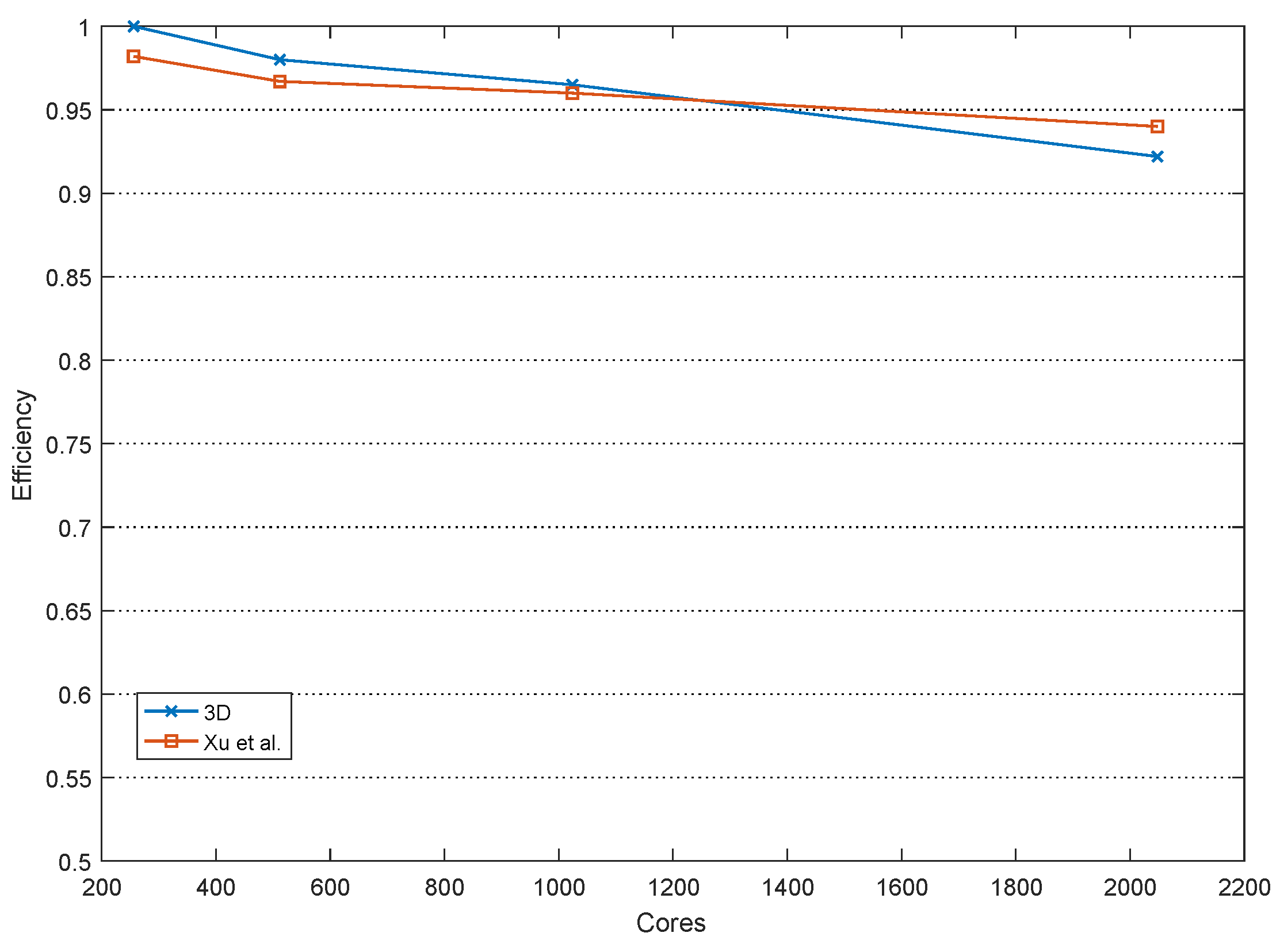
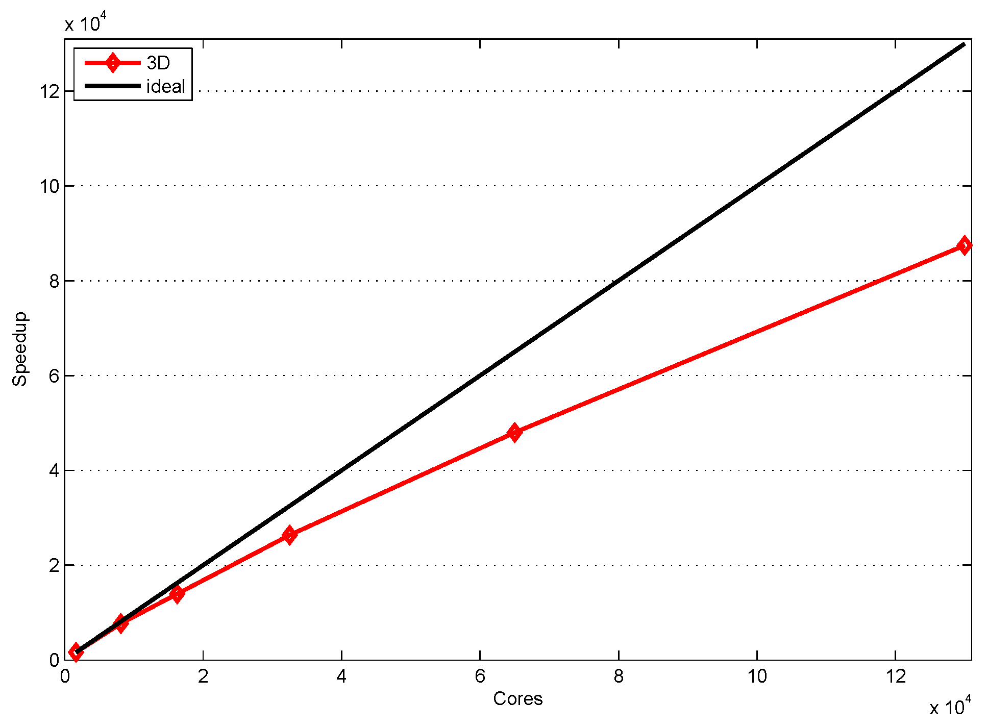
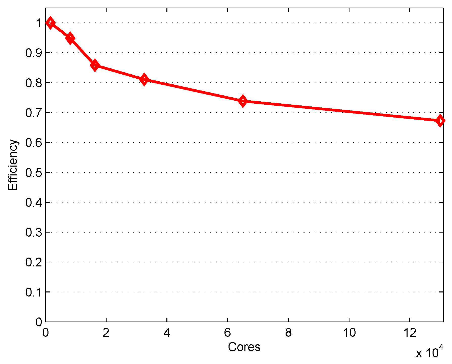
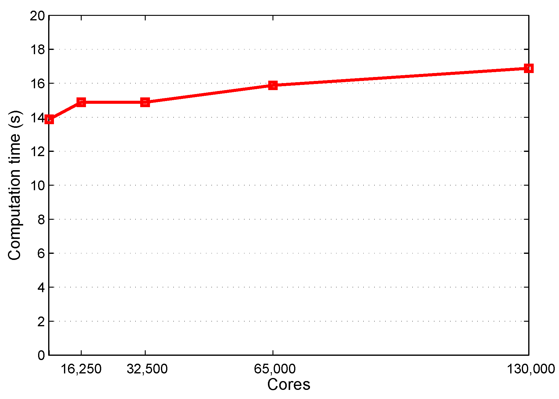
4.3. Performance of 3D Domain Decomposition on Hundreds of Thousands of Cores

The simulation was carried out on Sunway BlueLight MPP supercomputer in National Supercomputing Center in Jinan. Sunway BlueLight MPP consists of 8706 CPUs. The CPU model is SW1600, with 16 cores; the frequency is 1600 MHz; and each CPU is matched with 16 GB of DDR3 memory. Its peak speed is 1.07 Pflops/s, and its continuous speed is 795.9 Tflop/s.

Figure 24 and Figure 25 show the speedup and efficiency of 3D domain decomposition on a large-scale cluster, respectively. Figure 26 shows the weak scaling. It can be concluded that the proposed algorithms are still effective even on hundreds of thousands of cores. The parallel speedup and efficiency on large-scale computing clusters (Figure 24, Figure 25 and Figure 26) validate the load balancing capabilities and high scalability of RLBM parallel algorithms.

5. Conclusions

In this paper, we analyze the serial computing details of RLBM with LES in detail. Considering the architecture characteristics of the large-scale computing cluster, the highly scalable parallel algorithm with computing load balancing is proposed. This paper used the domain decomposition method to design three grid partition strategies, and introduced the buffer technology to provide the corresponding parallel data exchange strategy. MPI is used for parallel data exchange between computing nodes. The proposed parallel algorithm has the properties of computational load balancing and high scalability.

We used this parallel algorithm to simulate the flow of the 3D lid-driven cavity flow under the high Reynolds number, and compare with the results of Prasad et al. The experimental results show that RLBM with LES has a good stability under the high Reynolds number. When computing resources are relatively small, DDM decomposition along one direction is feasible. However, when the operating environment becomes a large cluster with hundreds of thousands of cores, the three-dimensional decomposition is reasonable and efficient. By analyzing the experimental results calculated on Shanghai University’s “Ziqiang 4000” and Sunway BlueLight MPP in NSCC-JN, we prove that the effect of 3D decomposition is the best and the presented algorithms are efficient and scalable. It is foreseeable that even on one million CPU cores, the speedup ratio will not drop significantly.

In the field of HPC, integrating parallel algorithms with Multigrid techniques is crucial, especially in LES turbulence modeling. The multigrid method, a sophisticated hierarchical approach, excels in solving LES equations on multiple grid levels, ensuring rapid convergence in turbulent flow simulations. Its adaptability is vital in understanding complex turbulence phenomena within LES. Moreover, the parallel algorithms of RLBM and LES under multi-layer mesh will be studied in depth in the future work.

The challenge in using multiple GPUs lies in efficient communication. Within a single node, communication is easier and more efficient. However, when GPUs span multiple nodes, factors such as grid partitioning and communication strategies complicate matters. Achieving a high efficiency in cross-node GPU communication is difficult and requires careful planning and strategic implementation of communication methods and computational coordination. Despite challenges in adapting our proposed parallel algorithm to heterogeneous CPU-GPU platforms, future efforts will refine our approach for multi-GPU or multi-MIC configurations in LES simulations. These endeavors will optimize the synergy between parallel algorithms and the Multigrid framework, not only in LES but also exploring integrations with other turbulence models, such as Reynolds stress models or detached eddy simulation. This pursuit promises advanced solutions for large-scale LES simulations, marking a significant step in this evolving computational field.

References

1. Godunov, S.K.; Bohachevsky, I. Finite difference method for numerical computation of discontinuous solutions of the equations of fluid dynamics. Mat. Sb. 1959, 47, 271–306. [Google Scholar]
2. Eymard, R.; Gallouët, T.; Herbin, R. Finite volume methods. Handb. Numer. Anal. 2000, 7, 713–1018. [Google Scholar]
3. Zienkiewicz, O.C.; Taylor, R.L.; Zhu, J.Z. The Finite Element Method: Its Basis and Fundamentals; Elsevier: Amsterdam, The Netherlands, 2005. [Google Scholar]
4. Canuto, C.; Hussaini, M.Y.; Quarteroni, A.; Zang, T. Spectral Methods: Evolution to Complex Geometries and Applications to Fluid Dynamics; Springer Science & Business Media: Berlin/Heidelberg, Germany, 2007. [Google Scholar]
5. Ullah, I. Activation energy with exothermic/endothermic reaction and Coriolis force effects on magnetized nanomaterials flow through Darcy–Forchheimer porous space with variable features. Waves Random Complex Media 2022, 1–14. [Google Scholar] [CrossRef]
6. Ullah, I. Heat transfer enhancement in Marangoni convection and nonlinear radiative flow of gasoline oil conveying Boehmite alumina and aluminum alloy nanoparticles. Int. Commun. Heat Mass Transf. 2022, 132, 105920. [Google Scholar]
7. Ullah, S.; Ullah, I.; Ali, A. Soret and Dufour effects on dissipative Jeffrey nanofluid flow over a curved surface with nonlinear slip, activation energy and entropy generation. Waves Random Complex Media 2023, 1–23. [Google Scholar] [CrossRef]
8. Ullah, I.; Alam, M.M.; Shah, M.I.; Weera, W. Marangoni convection in dissipative flow of nanofluid through porous space. Sci. Rep. 2023, 13, 6287. [Google Scholar] [CrossRef] [PubMed]
9. Ullah, I.; Shukat, S.; Albakri, A.; Khan, H.; Galal, A.M.; Jamshed, W. Thermal performance of aqueous alumina–titania hybrid nanomaterials dispersed in rotating channel. Int. J. Mod. Phys. B 2023, 37, 2350237. [Google Scholar] [CrossRef]
10. Hollingsworth, S.A.; Dror, R.O. Molecular dynamics simulation for all. Neuron 2018, 99, 1129–1143. [Google Scholar]
11. Wolfram, S. Cellular automata as models of complexity. Nature 1984, 311, 419–424. [Google Scholar] [CrossRef]
12. Cheng, X.; Su, R.; Shen, X.; Deng, T.; Zhang, D.; Chang, D.; Zhang, B.; Qiu, S. Modeling of indoor airflow around thermal manikins by multiple-relaxation-time lattice Boltzmann method with LES approaches. Numer. Heat Transf. Part A Appl. 2020, 77, 215–231. [Google Scholar]
13. Silva, G. Consistent lattice Boltzmann modeling of low-speed isothermal flows at finite Knudsen numbers in slip-flow regime. II. Application to curved boundaries. Phys. Rev. E 2018, 98, 023302. [Google Scholar] [CrossRef] [PubMed]
14. Wang, H.; Liu, H. A mesoscopic coupling scheme for solute transport in surface water using the lattice boltzmann method. J. Hydrol. 2020, 588, 125062. [Google Scholar] [CrossRef]
15. Saboohi, Z.; Roofeh, S.; Salimi, M. Analysis of misalignment effects on hydrodynamic non-circular journal bearings using three-dimensional lattice boltzmann method. Iran. J. Sci. Technol. Trans. A Sci. 2020, 44, 1739–1751. [Google Scholar] [CrossRef]
16. Wu, W.; Liu, X.; Dai, Y.; Li, Q. An in-depth quantitative analysis of wind turbine blade tip wake flow based on the lattice Boltzmann method. Environ. Sci. Pollut. Res. 2021, 28, 40103–40115. [Google Scholar] [CrossRef] [PubMed]
17. Jiang, F.; Liu, H.; Chen, X.; Tsuji, T. A coupled LBM-DEM method for simulating the multiphase fluid-solid interaction problem. J. Comput. Phys. 2022, 454, 110963. [Google Scholar]
18. Berra, E.M.; Faraji, M. Lattice Boltzmann Method Investigations of Natural Convection within a Cavity Equipped with a Heat Source: A Parametric Study. Heat Transf. Res. 2022, 53, 71–99. [Google Scholar] [CrossRef]
19. Afra, B.; Karimnejad, S.; Delouei, A.A.; Tarokh, A. Flow control of two tandem cylinders by a highly flexible filament: Lattice spring IB-LBM. Ocean Eng. 2022, 250, 111025. [Google Scholar]
20. Delouei, A.A.; Karimnejad, S.; He, F. Direct Numerical Simulation of pulsating flow effect on the distribution of non-circular particles with increased levels of complexity: IB-LBM. Comput. Math. Appl. 2022, 121, 115–130. [Google Scholar]
21. Chen, S.; Chen, H.; Martnez, D.; Matthaeus, W. Lattice Boltzmann model for simulation of magnetohydrodynamics. Phys. Rev. Lett. 1991, 67, 3776. [Google Scholar] [CrossRef]
22. Simonis, S.; Oberle, D.; Gaedtke, M.; Jenny, P.; Krause, M.J. Temporal large eddy simulation with lattice Boltzmann methods. J. Comput. Phys. 2022, 454, 110991. [Google Scholar] [CrossRef]
23. Sun, H.; Jiang, L.; Xia, Y. LBM simulation of non-Newtonian fluid seepage based on fractional-derivative constitutive model. J. Pet. Sci. Eng. 2022, 213, 110378. [Google Scholar]
24. Ezzatneshan, E. Comparative study of the lattice Boltzmann collision models for simulation of incompressible fluid flows. Math. Comput. Simul. 2019, 156, 158–177. [Google Scholar]
25. Latt, J.; Chopard, B. Lattice Boltzmann method with regularized pre-collision distribution functions. Math. Comput. Simul. 2006, 72, 165–168. [Google Scholar] [CrossRef]
26. Smagorinsky, J. General circulation experiments with the primitive equations: I. The basic experiment. Mon. Weather Rev. 1963, 91, 99–164. [Google Scholar] [CrossRef]
27. Hou, S.; Sterling, J.; Chen, S.; Doolen, G. A lattice Boltzmann subgrid model for high Reynolds number flows. Pattern Form. Lattice Gas Autom. 1995, 151–166. [Google Scholar]
28. Tiftikçi, A.; Kocar, C. Lattice Boltzmann simulation of flow across a staggered tube bundle array. Nucl. Eng. Des. 2016, 300, 135–148. [Google Scholar]
29. Mekala, M.; Dhiman, G.; Srivastava, G.; Nain, Z.; Zhang, H.; Viriyasitavat, W.; Varma, G. A DRL-based service offloading approach using DAG for edge computational orchestration. IEEE Trans. Comput. Soc. Syst. 2022. Early Access. [Google Scholar]
30. Shukla, S.K.; Gupta, V.K.; Joshi, K.; Gupta, A.; Singh, M.K. Self-aware execution environment model (SAE2) for the performance improvement of multicore systems. Int. J. Mod. Res. 2022, 2, 17–27. [Google Scholar]
31. Vaishnav, P.K.; Sharma, S.; Sharma, P. Analytical review analysis for screening COVID-19 disease. Int. J. Mod. Res. 2021, 1, 22–29. [Google Scholar]
32. Chatterjee, I. Artificial intelligence and patentability: Review and discussions. Int. J. Mod. Res. 2021, 1, 15–21. [Google Scholar]
33. Gupta, V.K.; Shukla, S.K.; Rawat, R.S. Crime tracking system and people’s safety in India using machine learning approaches. Int. J. Mod. Res. 2022, 2, 1–7. [Google Scholar]
34. Sharma, T.; Nair, R.; Gomathi, S. Breast cancer image classification using transfer learning and convolutional neural network. Int. J. Mod. Res. 2022, 2, 8–16. [Google Scholar]
35. Alferaidi, A.; Yadav, K.; Alharbi, Y.; Razmjooy, N.; Viriyasitavat, W.; Gulati, K.; Kautish, S.; Dhiman, G. Distributed deep CNN-LSTM model for intrusion detection method in IoT-based vehicles. Math. Probl. Eng. 2022, 2022, 3424819. [Google Scholar] [CrossRef]
36. Puri, T.; Soni, M.; Dhiman, G.; Ibrahim Khalaf, O.; Alazzam, M.; Raza Khan, I. Detection of emotion of speech for RAVDESS audio using hybrid convolution neural network. J. Healthc. Eng. 2022, 2022, 8472947. [Google Scholar] [CrossRef]
37. Sharma, S.; Gupta, S.; Gupta, D.; Juneja, S.; Gupta, P.; Dhiman, G.; Kautish, S. Deep learning model for the automatic classification of white blood cells. Comput. Intell. Neurosci. 2022, 2022, 7384131. [Google Scholar] [CrossRef]
38. Swain, S.; Bhushan, B.; Dhiman, G.; Viriyasitavat, W. Appositeness of optimized and reliable machine learning for healthcare: A survey. Arch. Comput. Methods Eng. 2022, 29, 3981–4003. [Google Scholar]
39. Uppal, M.; Gupta, D.; Juneja, S.; Dhiman, G.; Kautish, S. Cloud-based fault prediction using IoT in office automation for improvisation of health of employees. J. Healthc. Eng. 2021, 2021, 8106467. [Google Scholar] [CrossRef]
40. Kumar, R.; Dhiman, G. A comparative study of fuzzy optimization through fuzzy number. Int. J. Mod. Res. 2021, 1, 1–14. [Google Scholar]
41. Xu, L.; Song, A.; Zhang, W. Scalable parallel algorithm of multiple-relaxation-time lattice Boltzmann method with large eddy simulation on multi-GPUs. Sci. Program. 2018, 2018, 1298313. [Google Scholar] [CrossRef]
42. Abas, A.; Mokhtar, N.H.; Ishak, M.H.H.; Abdullah, M.Z.; Ho Tian, A. Lattice Boltzmann model of 3D multiphase flow in artery bifurcation aneurysm problem. Comput. Math. Methods Med. 2016, 2016, 6143126. [Google Scholar]
43. Tan, J.; Sinno, T.R.; Diamond, S.L. A parallel fluid–solid coupling model using LAMMPS and Palabos based on the immersed boundary method. J. Comput. Sci. 2018, 25, 89–100. [Google Scholar]
44. Závodszky, G.; Paál, G. Validation of a lattice Boltzmann method implementation for a 3D transient fluid flow in an intracranial aneurysm geometry. Int. J. Heat Fluid Flow 2013, 44, 276–283. [Google Scholar] [CrossRef]
45. Basha, M.; Sidik, N.A.C. Numerical predictions of laminar and turbulent forced convection: Lattice Boltzmann simulations using parallel libraries. Int. J. Heat Mass Transf. 2018, 116, 715–724. [Google Scholar] [CrossRef]
46. Safdari Shadloo, M. Numerical simulation of compressible flows by lattice Boltzmann method. Numer. Heat Transf. Part A Appl. 2019, 75, 167–182. [Google Scholar] [CrossRef]
47. Jahidul Haque, M.; Mamun Molla, M.; Amirul Islam Khan, M.; Ahsan, K. Graphics process unit accelerated lattice Boltzmann simulation of indoor air flow: Effects of sub-grid scale model in large-eddy simulation. Proc. Inst. Mech. Eng. Part C J. Mech. Eng. Sci. 2020, 234, 4024–4040. [Google Scholar] [CrossRef]
48. Delbosc, N.; Summers, J.L.; Khan, A.; Kapur, N.; Noakes, C.J. Optimized implementation of the Lattice Boltzmann Method on a graphics processing unit towards real-time fluid simulation. Comput. Math. Appl. 2014, 67, 462–475. [Google Scholar] [CrossRef]
49. Zhao-Li, G.; Chu-Guang, Z.; Bao-Chang, S. Non-equilibrium extrapolation method for velocity and pressure boundary conditions in the lattice Boltzmann method. Chin. Phys. 2002, 11, 366. [Google Scholar] [CrossRef]
50. Obrecht, C.; Kuznik, F.; Tourancheau, B.; Roux, J.J. Multi-GPU implementation of the lattice Boltzmann method. Comput. Math. Appl. 2013, 65, 252–261. [Google Scholar] [CrossRef]
51. Lee, Y.H.; Huang, L.M.; Zou, Y.S.; Huang, S.C.; Lin, C.A. Simulations of turbulent duct flow with lattice Boltzmann method on GPU cluster. Comput. Fluids 2018, 168, 14–20. [Google Scholar] [CrossRef]
52. Schneider, P.; Eberly, D.H. Geometric Tools for Computer Graphics (Morgan Kaufmann Series in Computer Graphics and Geometric Modeling); Morgan Kaufmann Publishers: Burlington, MA, USA, 2003. [Google Scholar]
53. Ku, H.C.; Hirsh, R.S.; Taylor, T.D. A pseudospectral method for solution of the three-dimensional incompressible Navier-Stokes equations. J. Comput. Phys. 1987, 70, 439–462. [Google Scholar] [CrossRef]
54. Jiang, B.N.; Lin, T.; Povinelli, L.A. Large-scale computation of incompressible viscous flow by least-squares finite element method. Comput. Methods Appl. Mech. Eng. 1994, 114, 213–231. [Google Scholar] [CrossRef]
55. Prasad, A.K.; Koseff, J.R. Reynolds number and end-wall effects on a lid-driven cavity flow. Phys. Fluids A Fluid Dyn. 1989, 1, 208–218. [Google Scholar] [CrossRef]
56. Mei, R.; Yu, D.; Shyy, W.; Luo, L.S. Force evaluation in the lattice Boltzmann method involving curved geometry. Phys. Rev. E 2002, 65, 041203. [Google Scholar] [CrossRef] [PubMed]
57. Tiwari, S.S.; Pal, E.; Bale, S.; Minocha, N.; Patwardhan, A.W.; Nandakumar, K.; Joshi, J.B. Flow past a single stationary sphere, 1. Experimental and numerical techniques. Powder Technol. 2020, 365, 115–148. [Google Scholar] [CrossRef]
58. Turton, R.; Levenspiel, O. A short note on the drag correlation for spheres. Powder Technol. 1986, 47, 83–86. [Google Scholar] [CrossRef]
59. Xu, C.; Wang, X.; Li, D.; Che, Y.; Wang, Z. OpenMP4. 5-enabled large-scale heterogeneous Lattice Boltzmann multiphase flow simulations. In Proceedings of the 2019 IEEE Intl Conf on Parallel & Distributed Processing with Applications, Big Data & Cloud Computing, Sustainable Computing & Communications, Social Computing & Networking (ISPA/BDCloud/SocialCom/SustainCom), Xiamen, China, 16–18 December 2019; pp. 1007–1016. [Google Scholar]
60. Liu, Z.; Li, Y.; Song, W. Regularized lattice Boltzmann method parallel model on heterogeneous platforms. Concurr. Comput. Pract. Exp. 2022, 34, e6875. [Google Scholar] [CrossRef]
Figure 1. Velocity vectors in the D3Q19 model.
Applsci 13 11078 g001
Figure 2. Illustration of Curved Boundary.
Applsci 13 11078 g002
Figure 3. Flow chart of RLBM.
Applsci 13 11078 g003
Figure 4. Domain decomposition.
Applsci 13 11078 g004
Figure 5. One-dimensional data exchange along x direction.
Applsci 13 11078 g005
Figure 6. Two-dimensional surfaces of data exchange.
Applsci 13 11078 g006
Figure 7. Three-dimensional surfaces of data exchange.
Applsci 13 11078 g007
Figure 8. Three-dimensional edges of data exchange.
Applsci 13 11078 g008
Figure 9. Three-dimensional lid-driven cavity flow.
Applsci 13 11078 g009
Figure 10. Comparison with benchmark values for (a) v velocity at y = 0.5 [53]; (b) u velocity at x = 0.5 at Re = 100 and SAR = 1:1 [53,54].
Applsci 13 11078 g010
Figure 11. Comparison with benchmark values for (a) v velocity at y = 0.5 [53]; (b) u velocity at x = 0.5 at Re = 400 and SAR = 1:1 [53,54].
Applsci 13 11078 g011
Figure 12. Comparison with benchmark values for (a) v velocity at y = 0.5 [53]; (b) u velocity at x = 0.5 at Re = 1000, and SAR = 1:1 [53,54].
Applsci 13 11078 g012
Figure 13. Compariso n with benchmark values for (a) v velocity at y = 0.5, (b) u velocity at x = 0.5 at Re = 3200, and SAR = 0.5:1.
Applsci 13 11078 g013
Figure 14. Comparison with benchmark values for (a) v velocity at y = 0.5, (b) u velocity at x = 0.5 at Re = 5000, and SAR = 0.5:1.
Applsci 13 11078 g014
Figure 15. Comparison with benchmark values for (a) v velocity at y = 0.5, (b) u velocity at x = 0.5 at Re = 7500, and SAR = 0.5:1.
Applsci 13 11078 g015
Figure 16. Comparison with benchmark values for (a) v velocity at y = 0.5, (b) u velocity at x = 0.5 at Re = 10,000, and SAR = 0.5:1.
Applsci 13 11078 g016
Figure 17. Schematic diagram of three-dimensional flow past a circular cylinder.
Applsci 13 11078 g017
Figure 18. Drag force coefficient.
Applsci 13 11078 g018
Figure 19. Vortical structure, Re = 1000.
Applsci 13 11078 g019
Figure 20. Vortical structure, Re = 3700.
Applsci 13 11078 g020
Figure 21. Speedup comparison among three kinds of DDMs.
Applsci 13 11078 g021
Figure 22. Efficiency comparison among three kinds of DDMs.
Applsci 13 11078 g022
Figure 23. Compared with the results of Xu et al. [59].
Applsci 13 11078 g023
Figure 24. Speedup of 3D domain decomposition on hundreds of thousands of cores.
Applsci 13 11078 g024
Figure 25. Efficiency of 3D domain decomposition on hundreds of thousands of cores.
Applsci 13 11078 g025
Figure 26. Weak scaling (scaleup) on hundreds of thousands of cores. The global simulation domain increases proportionally to the number of cores.
Applsci 13 11078 g026