Adaptive Marginal Multi-Target Bayes Filter without Need for Clutter Density for Object Detection and Tracking

Abstract

The random finite set (RFS) approach for multi-target tracking is widely researched because it has a rigorous theoretical basis. However, many prior parameters such as the clutter density, survival probability and detection probability of the target, pruning threshold, merging threshold, initial state of the birth object and its error covariance matrix are required in the standard RFS-based filters. In real application scenes, it is difficult to obtain these prior parameters. To address this problem, an adaptive marginal multi-target Bayes filter without the need for clutter density is proposed. This filter obviates the need for prior clutter density and survival probability. Instead of using the prior initial states of newborn targets and their error covariance matrices, it uses two scans of observations to generate the initial states of potential birth targets and their error covariance matrices according to the least squares technique. Simulation results reveal that the proposed adaptive filter has smaller OSPA and OSPA⁽²⁾ errors as well as less cardinality error than the adaptive RFS-based filters. The OSPA and OSPA⁽²⁾ errors have been reduced by more than 20% compared to those of the adaptive RFS-based filters.

1. Introduction

Detecting the target and estimating its state at specific times are the major task of multi-target tracking (MTT). MTT has been widely used in civilian and military fields such as missile warning, air surveillance, air and ground traffic control, autonomous driving, etc. The challenge in radar MTT is the presence of clutter and noise and the uncertainty of data association [1,2,3,4,5,6,7]. Traditional radar MTT approaches are based on data association techniques and they have been used in different radar MTT systems for several decades [3,8,9]. Generally, the traditional radar MTT approaches detect the birth object and form its track according to the measurements from several different time steps, and associate the measurement with the existing object to maintain its track at each time step. With the establishment of the random finite set (RFS) theory [1] and labeled RFS theory, the probability hypothesis density (PHD) filter [10,11], cardinality-balanced multi-Bernoulli (CBMeMber) filter [12] and δ-generalized labeled multi-Bernoulli (δ-GLMB) filter [13,14,15] have been proposed to track multiple objects in the presence of clutter, missed detections, noise and uncertain data associations. These three tractable RFS-based filters are the approximate implementations of the optimal multi-object Bayes filter. They provide the three suboptimal solutions for the multi-object tracking problem. The defects of the CBMeMber filter [12] and the PHD filter [10,11] are that they require a high signal-to-noise ratio and that they cannot provide the target tracks. The δ-GLMB filter was proposed to overcome these defects [13,14,15]. Despite their advantage in theory, the δ-GLMB filter, CBMeMber filter and the PHD filter need many prior parameters. In order to acquire the predicted and updated intensity or density, the clutter density, survival probability and detection probability of the target are assumed to be known in these three RFS-based filters. Because each potential target (or Gaussian item) is associated with each observation at each time step in these three RFS-based filters, severely combinatorial explosion arises as the filtering recursion increases. The pruning threshold and merging threshold must be applied in these filters to restrict the combinatorial explosion [1]. In addition, the three RFS-based filters assume that the birth intensity or density is known a priori. This assumption also implies that initial states and error covariance matrices of targets are known in advance.

To obviate the need for the prior initial states or error covariance matrices of birth targets, the adaptive methods for forming the birth object intensity or density are discussed in [16,17,18,19,20,21,22]. The adaptive methods in [16,20,21] use the measurements of previous time steps to form the birth intensity or birth filtering density. In order to avoid the repeated use of measurements, the gating technique is needed in these approaches to remove the measurements near the current multi-target states [16,20]. However, these adaptive methods still require the known error covariance of birth targets. To obviate the need for the prior error covariance of birth targets, the adaptive methods in [17,18,19] use the measurements of the previous two time steps to build the potential birth track and then use the potential birth track to form the birth intensity or density. The adaptive δ-GLMB (AGLMB) filter [22] uses the measurements of the previous three time steps to build the tentative track based on the rule-based track initiation technique [23], and estimates the state of the tentative track and its error covariance according to the least squares technique.

However, the adaptive RFS-based filters still require that the clutter density and survival probability are known in advance. The clutter density and survival probability play important roles in obtaining the predicted and updated densities or intensities in the adaptive RFS-based filters, but it can be challenging to accurately estimate them in real-world scenarios. To track multiple objects in the presence of unknown clutter density, unknown survival probability, and unknown initial state and error covariance, we propose an adaptive marginal multi-target Bayes (AMTB) filter without the need for clutter density and survival probability in this paper. The filter delivers the probability density function (PDF), track label and existence probability of the object in the filtering recursion. Two data association steps are required in the recursion of this filter. The first data association step is employed to associate the measurements with the existing target. To do this, the AMTB filter first uses the gate technique to select the measurements falling inside the acceptance gates of individual existing targets from the measurements at time step $k$ and then employs the two-dimensional assignment technique to assign the selected observations to individual existing objects. If a measurement is assigned to an existing object, the updated PDF of this existing object that is correlated to this observation is used as its PDF. If no measurement is assigned to an existing object, its predicted PDF is used as its PDF. The second data association step is employed to associate the measurements with the potential birth target. To do this, the AMTB filter selects the measurements falling inside the acceptance gates of individual potential birth targets from the unused measurements at time step $k$ and then employs the two-dimensional assignment technique to assign the selected observations to individual potential birth objects. If a measurement is assigned to a potential birth target, this potential birth target becomes a newborn target. Moreover, this filter uses the unused observations at time steps $k-1$ and $k$ to form the potential birth targets in terms of the velocity, and uses the least squares technique to acquire the initial state of each potential birth target and its error covariance. Due to the use of the gating technique, the proposed filter obviates the need for prior clutter density, survival probability, initial state of the birth object and its error covariance. The simulation results demonstrate that the AMTB filter outperforms the AGLMB filter [22], adaptive CBMeMber (ACBMeMber) filter [20], adaptive multi-Bernoulli (AMB) filter [19] and adaptive PHD (APHD) filter [17].

Our contribution in this article is that we propose an adaptive marginal multi-target Bayes filter without the need for clutter density. The main advantage of the proposed filter over the available adaptive filters is that it obviates the need for clutter density and survival probability that are required for the available adaptive filters. Identical to adaptive RFS-based filters, the proposed filter is applied to radar MTT systems.

The structure of the article is as follows: the AMTB filter without the need for clutter density for a linear Gaussian noisy system is given in Section 2. An extension of this filter to nonlinear observations is provided in Section 3. The performance evaluation of the AMTB filter is given in Section 4 by comparing it with adaptive RFS-based filters. In Section 5, we provide the conclusions.

2. AMTB Filter without Need for Clutter Density

The object dynamic and observation models are defined as:

$$x_k={\Phi }_{k-1}{x}_{k-1}+w_{k-1}$$

(1)

$$z_k=H_k{x}_k+v_k$$

(2)

where $x_k$ and $z_k$ are the state and observation vectors; ${\Phi }_{k-1}$ and $H_k$ are the state transition and observation matrices; and $w_{k-1}$ and $v_k$ are the zero-mean Gaussian process and observation noises where $Q_{k-1}$ and $R_k$ are their covariance matrices.

The AMTB filter without the need for clutter density propagates the track labels, existence probabilities of objects and their PDFs. We assume that the set of existing objects and the set of potential birth objects at time step $k-1$ are

$${\left\{r_{i,k-1}^e,N(x_{i,k-1}^{};m_{i,k-1}^e,P_{i,k-1}^e),{\ell }_{i,k-1}^e\right\}}_{i=1}^{N_{k-1}^e}$$

(3)

$${\left\{{\epsilon }_{i,k-1},m_{i,k-2}^b,N(x_{i,k-1}^{};m_{i,k-1}^b,P_{i,k-1}^b)\right\}}_{i=1}^{N_{k-1}^b}$$

(4)

where ${\mathit{x}}_{i,k-1}$ denotes the state vector of object $i$ at time step $k-1$; $N_{k-1}^e$, ${\ell }_{i,k-1}^e$ and $r_{i,k-1}^e$ denote the number of existing objects, track label and existence probability of existing object $i$, respectively; ${\epsilon }_{i,k-1}$, ${\ell }_{i,k-1}^b$ and $N_{k-1}^b$ are the index of the relative measurement with potential birth object $i$, track label of potential birth object $i$ and number of potential birth objects at time step $k-1$, respectively; and $m_{i,k-2}^b$ denotes the mean vector of potential birth object $i$ at time step $k-2$. The PDFs of the existing object and potential birth object are assumed to be Gaussian and they are given by $N(x_{i,k-1}^{};m_{i,k-1}^e,P_{i,k-1}^e)$ and $N(x_{i,k-1}^{};m_{i,k-1}^b,P_{i,k-1}^b)$, respectively, where $m_{i,k-1}^e$ and $m_{i,k-1}^b$ are the mean vector, and $P_{i,k-1}^e$ and $P_{i,k-1}^b$ are error covariance matrices. The recursion of the ATMB filter without the need for clutter density is as follows:

2.1. Prediction

In terms of (1) and (3), the set of predicted existing objects is:

$${\left\{r_{i,k|k-1}^e,N(x_{i,k}^{};m_{i,k|k-1}^e,P_{i,k|k-1}^e),{\ell }_{i,k|k-1}^e\right\}}_{i=1}^{N_{k-1}^e}$$

(5)

where

$$r_{i,k|k-1}^e=r_{i,k-1}^e, m_{i,k|k-1}^e={\Phi }_{k-1}^{}{m}_{i,k-1}^e, P_{i,k|k-1}^e={\Phi }_{k-1}{P}_{i,k-1}^e{\Phi }_{k-1}^{\mathrm{T}}+Q_{k-1}, {\ell }_{i,k|k-1}^e={\ell }_{i,k-1}^e$$

(6)

In terms of (1) and (4), the set of predicted potential birth objects is:

$${\left\{N(x_{i,k}^{};m_{i,k|k-1}^b,P_{i,k|k-1}^b)\right\}}_{i=1}^{N_{k-1}^b}$$

(7)

where

$$m_{i,k|k-1}^b={\Phi }_{k-1}^{}{m}_{i,k-1}^b, P_{i,k|k-1}^b={\Phi }_{k-1}{P}_{i,k-1}^b{\Phi }_{k-1}^{\mathrm{T}}+Q_{k-1}$$

(8)

In terms of (2) and (5), the predicted measurement vector of the existing target and its error covariance matrix are:

$$z_{i,k|k-1}^e=H_k{m}_{i,k|k-1}^e, S_{i,k}^e=H_k{P}_{i,k|k-1}^e{\left(H_k\right)}^T$$

(9)

In terms of (2) and (7), the predicted measurement vector of the potential birth target and its error covariance matrix are:

$$z_{i,k|k-1}^b=H_k{m}_{i,k|k-1}^b, S_{i,k}^b=H_k{P}_{i,k|k-1}^b{\left(H_k\right)}^T$$

(10)

2.2. Update of Existing Objects

In this step, we associate the observations at step $k$ with the existing targets. The existence of an object is confirmed and its state is updated if a measurement is assigned to it. An object is not detected if no measurement is assigned to it, and its state is given by its predicted state.

The Mahalanobis distance is used to measure the correlation between the target and the measurement, and denoting the measurement set at time step $k$ by $y_k={\left\{z_{j,k}^{}\right\}}_{j=1}^{M_k}$ where $M_k$ is the observation number. The Mahalanobis distance between measurement $z_{j,k}^{}$ and existing object $i$ may be given by:

$$q_{ij}^e={(z_{j,k}^{}-z_{i,k|k-1}^e)}^{\mathrm{T}}{\left(S_{i,k}^e+R_k^{}\right)}^{-1}(z_{j,k}^{}-z_{i,k|k-1}^e)$$

(11)

$q_{ij}^e$ follows a chi-square distribution, and its degree of freedom equals the dimension of observation $z_{j,k}^{}$. An acceptance threshold $q_{\alpha }$ may be determined in terms of the chi-square distribution table after giving a confidence level $\alpha$. If $q_{ij}^e<q_{\alpha }^{}$, we confirm that $z_{j,k}^{}$ falls in the acceptance gate of existing target $i$.

To avoid the track splitting, we use the 2-dimensional assignment to associate the measurement with the existing target. The cost matrix for the 2-dimensional assignment is:

$$C=\left[\begin{array}{cc}{C}_1& C_2\end{array}\right]$$

(12)

where

$$C_1={\left[q_{ij}^e\right]}_{N_{k-1}^e\times M_k^{}}=\left[\begin{array}{cccc}{q}_{11}^e& q_{12}^e& \cdots & q_{1,M_k^{}}^e\\ q_{21}^e& q_{22}^e& \cdots & q_{2,M_k^{}}^e\\ ⋮& ⋮& \ddots & ⋮\\ q_{N_{k-1}^e,1}^e& q_{N_{k-1}^e,2}^e& \cdots & q_{N_{k-1}^e,M_k^{}}^e\end{array}\right], C_2={\left[\begin{array}{cccc}{q}_{\alpha }& \infty & \cdots & \infty \\ \infty & q_{\alpha }& \cdots & \infty \\ ⋮& ⋮& \ddots & ⋮\\ \infty & \infty & \cdots & q_{\alpha }\end{array}\right]}_{N_{k-1}^e\times N_{k-1}^e}$$

(13)

According to $C$, we acquire an optimal solution with the minimum cost by using the optimized Murty algorithm [24]. The optimal solution can be given as:

$$\mathsf{\Theta }=\left[{\theta }_1,{\theta }_2,\cdots ,{\theta }_{N_{k-1}^e}\right]$$

(14)

where ${\theta }_i^{}\in \left\{1,2,\cdots ,M_k^{}+N_{k-1}^e\right\}$ for $i=1,2,\cdots ,N_{k-1}^e$. $1\le {\theta }_i\le M_k$ demonstrates that $z_{{\theta }_i,k}^{}$ is assigned to existing object $i$, while ${\theta }_i>M_k$ reveals that no measurement is assigned to existing object $i$.

To detect the potential birth objects and form newborn tracks, the proposed filter needs a set of unused measurements. We use binary variable $g_{j,k}$ to denote whether measurement $z_{j,k}$ is used or not, and set $g_{j,k}=0$ for $j=1,2,\cdots ,M_k$.

If $1\le {\theta }_i\le M_k$, we set $j={\theta }_i^{}$ and use observation $z_{j,k}^{}$ to update the predicted PDF of object $i$. The PDF of object $i$ at time step $k$ can be given by:

$$N(x_{i,k}^{};m_{i,k}^e,P_{i,k}^e)=N(x_{i,k}^{};m_{ij}^e,P_{ij}^e)$$

(15)

where

$$m_{ij}^e=m_{i,k|k-1}^e+A_i^e\cdot [z_{j,k}^{}-m_{i,k|k-1}^e]$$

(16)

$$P_{ij}^e=P_{i,k|k-1}^e-A_i^e{H}_k{P}_{i,k|k-1}^e$$

(17)

$$A_i^e=P_{i,k|k-1}^e{\left(H_k\right)}^{\mathrm{T}}{[H_k{P}_{i,k|k-1}^e{\left(H_k\right)}^{\mathrm{T}}+R_k]}^{-1}$$

(18)

In this case, its existence probability is:

$$r_{i,k}^e=1$$

(19)

Since measurement $z_{j,k}^{}$ is used, $g_{j,k}$ is updated by:

$$g_{j,k}=1$$

(20)

If ${\theta }_i^{}>M_k$, object $i$ is not detected because no observation is assigned to it. Its PDF at time step $k$ can be given by its predicted PDF as:

$$N(x_{i,k}^{};m_{i,k}^e,P_{i,k}^e)=N(x_{i,k}^{};m_{i,k|k-1}^e,P_{i,k|k-1}^e)$$

(21)

Using $p_D^{}$ to denote the detection probability, the existence probability of object $i$ is as follows:

$$r_{i,k}^e=(1-p_D^{})r_{i,k|k-1}^e$$

(22)

No matter whether existing object $i$ is detected, its track label can be given by:

$${\ell }_{i,k}^e={\ell }_{i,k|k-1}^e$$

(23)

After dealing with the optimal solution, the set of the existing objects can be given by:

$${\left\{r_{i,k}^e,N(x_{i,k}^{};m_{i,k}^e,P_{i,k}^e),{\ell }_{i,k}^e\right\}}_{i=1}^{N_{k-1}^e}$$

(24)

The set of unused observations at time step $k$ is given by:

$$Z_k^u=\left\{z_{j,k}^{}|g_{j,k}=0\right\}$$

(25)

Algorithm 1 gives the pseudo-code for updating existing objects.

Algorithm 1 Update of existing objects

1: for $i=1:N_{k-1}^e$ 2:  for $j=1:M_k$ 3:   $q_{ij}^e={(z_{j,k}^{}-z_{i,k|k-1}^e)}^{\mathrm{T}}{\left(S_{i,k}^e+R_k^{}\right)}^{-1}(z_{j,k}^{}-z_{i,k|k-1}^e)$. 4:  end for 5: end for 6: Form cost matrix $C$ in terms of (12) and (13). 7: Acquire an optimal solution $\mathsf{\Theta }=\left[{\theta }_1,{\theta }_2,\cdots ,{\theta }_{N_{k-1}^e}\right]$ according to $C$. 8: Set $Z_k^u=$Ø; and $g_{j,k}=0$ for $j=1,2,\cdots ,M_k$. 9: for $i=1:N_{k-1}^e$ 10:  if $1\le {\theta }_i\le M_k$ 11:   $j={\theta }_i$, $r_{i,k}^e=1$, $A_i^e=P_{i,k|k-1}^e{\left(H_k\right)}^{\mathrm{T}}{[H_k{P}_{i,k|k-1}^e{\left(H_k\right)}^{\mathrm{T}}+R_k]}^{-1}$, 12:   $m_{i,k}^e=m_{i,k|k-1}^e+A_i^e\cdot [z_{j,k}^{}-m_{i,k|k-1}^e]$, $P_{i,k}^e=P_{i,k|k-1}^e-A_i^e{H}_k{P}_{i,k|k-1}^e$, $g_{j,k}=1$. 13:  else 14:   $m_{i,k}^e=m_{i,k|k-1}^e$, $P_{i,k}^e=P_{i,k|k-1}^e$, $r_{i,k}^e=(1-p_D^{})r_{i,k|k-1}^e$. 15:  end if 16:  ${\ell }_{i,k}^e={\ell }_{i,k|k-1}^e$ 17: end for 18: for $j=1:M_k^{}$ 19:  if $g_{j,k}=0$ 20:   $Z_k^u=[Z_k^u z_{j,k}^{}]$ 21:  end if 22: end for 23: Output: ${\left\{r_{i,k}^e,m_{i,k}^e,P_{i,k}^e,{\ell }_{i,k}^e\right\}}_{i=1}^{N_{k-1}^e},$$Z_k^u$.

2.3. Establishment of Newborn Objects

In this step, we associate the unused observations at step $k$ with the potential birth objects. A newborn object is established if a measurement is assigned to a potential birth object.

Let $Z_k^u={\left\{z_{g,k}^u\right\}}_{g=1}^{M_k^u}$ denote a set of unused measurements where $M_k^u$ is the number of unused measurements. The Mahalanobis distance between unused measurement $z_{g,k}^u$ and potential birth object $i$ is:

$$q_{ig}^b={(z_{g,k}^u-z_{i,k|k-1}^b)}^{\mathrm{T}}{\left(S_{i,k}^b+R_k^{}\right)}^{-1}(z_{g,k}^u-z_{i,k|k-1}^b)$$

(26)

Identical to Section 2.2, we use the 2-dimensional assignment to associate the measurement with the potential birth object. The cost matrix for the 2-dimensional assignment is:

$$C=\left[\begin{array}{cc}{C}_1& C_2\end{array}\right]$$

(27)

where

$$C_1={\left[q_{ig}^b\right]}_{N_{k-1}^b\times M_k^u}=\left[\begin{array}{cccc}{q}_{11}^b& q_{12}^b& \cdots & q_{1,M_k^u}^b\\ q_{21}^b& q_{22}^b& \cdots & q_{2,M_k^u}^b\\ ⋮& ⋮& \ddots & ⋮\\ q_{N_{k-1}^b,1}^b& q_{N_{k-1}^b,2}^b& \cdots & q_{N_{k-1}^b,M_k^u}^b\end{array}\right], C_2={\left[\begin{array}{cccc}{q}_{\alpha }& \infty & \cdots & \infty \\ \infty & q_{\alpha }& \cdots & \infty \\ ⋮& ⋮& \ddots & ⋮\\ \infty & \infty & \cdots & q_{\alpha }\end{array}\right]}_{N_{k-1}^b\times N_{k-1}^b}$$

(28)

In terms of $C$, we can acquire an optimal solution with the minimum cost by using the optimized Murty algorithm [24]. The optimal solution can be given as:

$$\mathsf{\Theta }=\left[{\theta }_1,{\theta }_2,\cdots ,{\theta }_{N_{k-1}^b}\right]$$

(29)

where ${\theta }_i^{}\in \left\{1,2,\cdots ,M_k^u+N_{k-1}^b\right\}$ for $i=1,2,\cdots ,N_{k-1}^b$. $1\le {\theta }_i\le M_k^u$ demonstrates that $z_{{\theta }_i,k}^u$ is assigned to potential birth object $i$.

A newborn object is established if a measurement is assigned to a potential birth object. Since $1\le {\theta }_i\le M_k^u$ demonstrates that $z_{{\theta }_i,k}^u$ is assigned to potential birth object $i$, a newborn object $h$ is established according to potential birth object $i$ and measurement $z_{{\theta }_i,k}^u$. The PDF of newborn object $h$ is:

$$N(x_{h,k}^{};m_{h,k}^{},P_{h,k}^{})$$

(30)

where

$$m_{h,k}^{}=m_{i,k|k-1}^b+A_i^b\cdot [z_{{\theta }_i,k}^u-m_{i,k|k-1}^b]$$

(31)

$$P_{h,k}^{}=P_{i,k|k-1}^b-A_i^b{H}_k{P}_{i,k|k-1}^b$$

(32)

$$A_i^b=P_{i,k|k-1}^b{\left(H_k\right)}^{\mathrm{T}}{[H_k{P}_{i,k|k-1}^b{\left(H_k\right)}^{\mathrm{T}}+R_k]}^{-1}$$

(33)

The track label of newborn object $h$ and its existence probability are:

$${\ell }_{h,k}^{}=\left[\begin{array}{c}k\\ h\end{array}\right]; r_{h,k}^{}=1$$

(34)

The mean vectors of newborn object $h$ at time steps $k-2$ and $k-1$ are given by:

$$m_{h,k-2}^{}=m_{i,k-2}^b; m_{h,k-1}^{}=m_{i,k-1}^b$$

(35)

Since $z_{{\theta }_i,k}^u$ and $z_{{\epsilon }_{i,k-1},k-1}^u$ are used to establish newborn object $h$, they should be removed from sets $Z_k^u$ and $Z_{k-1}^u$ as:

$$Z_k^u=Z_k^u\backslash z_{{\theta }_i,k}^u, Z_{k-1}^u=Z_{k-1}^u\backslash z_{{\epsilon }_{i,k-1},k-1}^u$$

(36)

Dealing with each potential birth object according to optimal solution $\mathsf{\Theta }$, we can acquire a set of newborn objects and the updated sets $Z_k^u$ and $Z_{k-1}^u$. The set of newborn objects are:

$${\left\{r_{h,k}^{},N(x_{h,k}^{};m_{h,k}^{},P_{h,k}^{}),{\ell }_{h,k}^{}\right\}}_{h=1}^{N_k^a}$$

(37)

where $N_k^a$ is the number of newborn objects. We use the mean vectors of newborn objects and their track labels at time steps $k-2$, $k-1$ and $k$ to form three sets $X_{k-2}^b$, $X_{k-1}^b$ and $X_k^b$. The three sets are given by:

$$X_{k-2}^b={\left\{m_{h,k-2}^{},l_{h,k}^{}\right\}}_{h=1}^{N_k^a}, X_{k-1}^b={\left\{m_{h,k-1}^{},l_{h,k}^{}\right\}}_{h=1}^{N_k^a}, X_k^b={\left\{m_{h,k}^{},l_{h,k}^{}\right\}}_{h=1}^{N_k^a}$$

(38)

Algorithm 2 gives the pseudo-code for the establishment of newborn objects.

Algorithm 2 Establishment of newborn objects

1: for $i=1:N_{k-1}^b$ 2:  for $g=1:M_k^u$ 3:   $q_{ig}^b={(z_{g,k}^u-z_{i,k|k-1}^b)}^{\mathrm{T}}{\left(S_{i,k}^b+R_k^{}\right)}^{-1}(z_{g,k}^u-z_{i,k|k-1}^b)$. 4:  end for 5: end for 6: Establish cost matrix $C$ according to (27) and (28). 7: Acquire an optimal solution $\mathsf{\Theta }=\left[{\theta }_1,{\theta }_2,\cdots ,{\theta }_{N_{k-1}^b}\right]$ according to $C$. 8: Set $h=0$, $X_{k-2}^b=$ Ø, $X_{k-1}^b=$ Ø and $X_k^b=$ Ø. 9: for $i=1:N_{k-1}^e$ 10:  if $1\le {\theta }_i\le M_k^u$ 11:   $h=h+1$, $A_i^b=P_{i,k|k-1}^b{\left(H_k\right)}^{\mathrm{T}}{[H_k{P}_{i,k|k-1}^b{\left(H_k\right)}^{\mathrm{T}}+R_k]}^{-1}$. 12:   $m_{h,k}^{}=m_{i,k|k-1}^b+A_i^b\cdot [z_{{\theta }_i,k}^u-m_{i,k|k-1}^b]$, $P_{h,k}^{}=P_{i,k|k-1}^b-A_i^b{H}_k{P}_{i,k|k-1}^b$, $r_{h,k}^{}=1$, 13:   ${\ell }_{h,k}^{}=\left[\begin{array}{c}k\\ h\end{array}\right]$. 14:   $X_{k-2}^b=\left[X_{k-2}^b [m_{i,k-2}^b;{\ell }_{h,k}^{}]\right]$, $X_{k-1}^b=\left[X_{k-1}^b [m_{i,k-1}^b; {\ell }_{h,k}^{}]\right]$, 15:   $X_k^b=\left[X_k^b [m_{h,k}^{}; {\ell }_{h,k}^{}]\right]$. 16:   Remove $z_{{\theta }_i,k}^u$ and $z_{{\epsilon }_{i,k-1},k-1}^u$ from sets $Z_k^u$ and $Z_{k-1}^u$, respectively. 17:  end if 18: end for 19:$N_k^a=h$. 20: Output: ${\left\{r_{h,k}^{},m_{h,k}^{},P_{h,k}^{},{\ell }_{h,k}^{}\right\}}_{h=1}^{N_k^a}$, $Z_{k-1}^u$, $Z_k^u$, $X_{k-2}^b$,$X_{k-1}^b$, $X_k^b$.

2.4. Generation of Potential Birth Objects

In this step, we generate the potential birth objects based on the unused measurements at steps $k$ and $k-1$. A potential birth object is formed if the two picked measurements satisfy the given speed gating criterion.

Let $Z_{k-1}^u={\left\{z_{f,k-1}^u\right\}}_{f=1}^{M_{k-1}^u}$ and $Z_k^u={\left\{z_{g,k}^u\right\}}_{g=1}^{M_k^u}$ denote two sets of unused measurements at time steps $k-1$ and $k$. We pick observations $z_{f,k-1}^u$ and $z_{g,k}^u$ from sets $Z_{k-1}^u$ and $Z_k^u$, respectively, and then test whether they satisfy (39).

$$v_{\min }<\frac{{\Vert z_{g,k}^u-z_{f,k-1}^u\Vert }_2}{T}<v_{\max }$$

(39)

where $T$ is the scan period, and $v_{\min }$ and $v_{\max }$ are two speed thresholds. A potential birth object is detected if $z_{f,k-1}^u$ and $z_{g,k}^u$ satisfy (39). The mean vectors of the potential birth object at the time steps $k-1$ and $k$ according to the least squares technique [25] are:

$$m_{i,k-1}^b={({\mathsf{\Lambda }}_1^T{\mathsf{\Lambda }}_1)}^{-1}{\mathsf{\Lambda }}_1^T\left[\begin{array}{c}{z}_{f,k-1}^u\\ z_{g,k}^u\end{array}\right]$$

(40)

$$m_{i,k}^b={({\mathsf{\Lambda }}_2^T{\mathsf{\Lambda }}_2)}^{-1}{\mathsf{\Lambda }}_2^T\left[\begin{array}{c}{z}_{f,k-1}^u\\ z_{g,k}^u\end{array}\right]$$

(41)

where

$${\mathsf{\Lambda }}_1=\left[\begin{array}{cccc}1& 0& 0& 0\\ 0& 0& 1& 0\\ 1& T& 0& 0\\ 0& 0& 1& T\end{array}\right], {\mathsf{\Lambda }}_2=\left[\begin{array}{cccc}1& -T& 0& 0\\ 0& 0& 1& -T\\ 1& 0& 0& 0\\ 0& 0& 1& 0\end{array}\right]$$

(42)

Its error covariance at time steps $k$ is:

$$P_{i,k}^b={({\mathsf{\Lambda }}_2^T{\mathsf{\Lambda }}_2)}^{-1}{\mathsf{\Lambda }}_2^T\left[\begin{array}{cc}{R}_{k-1}& 0\\ 0& R_k^{}\end{array}\right]{\mathsf{\Lambda }}_2{({\mathsf{\Lambda }}_2^T{\mathsf{\Lambda }}_2)}^{-1}$$

(43)

Assume that potential birth object $i$ is generated based on measurements $z_{f,k-1}^u$ and $z_{g,k}^u$. This potential birth object is given by:

$$\left\{{\epsilon }_{i,k}^{}=g,m_{i,k-1}^b,N(x_{i,k};m_{i,k}^b,P_{i,k}^b)\right\}$$

(44)

where $g$ denotes the index of measurement $z_{g,k}^u$. ${\epsilon }_{i,k}^{}=g$ implies that measurement $z_{g,k}^u$ is used to form potential birth object $i$.

The set of potential birth objects can be acquired by repeating the above process and is given by:

$${\left\{{\epsilon }_{i,k}^{},m_{i,k-1}^b,N(x_{i,k};m_{i,k}^b,P_{i,k}^b)\right\}}_{i=1}^{N_k^b}$$

(45)

where $N_k^b$ denotes the number of potential birth objects.

Algorithm 3 gives the pseudo-code for the generation of potential birth objects.

Algorithm 3 Generation of potential birth objects

1:$i=0$ 2: for $f=1: M_{k-1}^u$ 3:  for $g=1: M_k^u$ 4:   if $v_{\min }<{\Vert z_{g,k}^u-z_{f,k-1}^u\Vert }_2/T<v_{\max }$ 5:    $i=i+1$ 6:    ${\epsilon }_{i,k}^{}=g$; Acquire $m_{i,k-1}^b,m_{i,k}^b$ and $P_{i,k}^b$ according to (40), (41) and (43). 7:   end if 8:  end for 9: end for 10:$N_k^b=i$. 11: Output: ${\left\{{\epsilon }_{i,k}^{},m_{i,k-1}^b,m_{i,k}^b,P_{i,k}^b\right\}}_{i=1}^{N_k^b}$.

2.5. Formation of Existing Objects

The surviving objects are acquired by picking the object with $r_{i,k}^e>{\tau }_r$ from the updated set of existing objects in (24) where ${\tau }_r$ is a given picking probability. We suggest that its value range is from 0.001 to 0.009. The set of acquired survival objects is:

$${\left\{r_{i,k}^e,N(x_{i,k}^{};m_{i,k}^e,P_{i,k}^e),{\ell }_{i,k}^e\right\}}_{i=1}^{N_k^s}$$

(46)

We use the mean vectors of survival objects and their track labels to form set $X_k^s$ as:

$$X_k^s={\left\{m_{i,k}^e,{\ell }_{i,k}^e\right\}}_{i=1}^{N_k^s}$$

(47)

where $N_k^s$ is the number of survival objects.

The existing objects include the survival objects and the newborn objects. The set of existing objects at time step $k$ can be acquired by combining the set of the newborn objects in (37) and the set of survival objects in (46) as:

$$\begin{array}{l}{\left\{r_{i,k}^e,N(x_{i,k}^{};m_{i,k}^e,P_{i,k}^e),{\ell }_{i,k}^e\right\}}_{i=1}^{N_k^e}\\ ={\left\{r_{i,k}^e,N(x_{i,k}^{};m_{i,k}^e,P_{i,k}^e),{\ell }_{i,k}^e\right\}}_{i=1}^{N_k^s}\cup {\left\{r_{h,k}^{},N(x_{h,k}^{};m_{h,k}^{},P_{h,k}^{}),{\ell }_{h,k}^{}\right\}}_{h=1}^{N_k^a}\end{array}$$

(48)

where $N_k^e=N_k^s+N_k^a$ is the number of existing objects at time step $k$. The set of existing objects in (48) and the set of potential birth objects in (45) along with unused measurement sets $Z_k^u$ are delivered to the next time step.

Combining set $X_k^s$ in (47) with the set in (38), we acquire set $X_k^{}$ as:

$$X_k^{}=X_k^s\cup X_k^b$$

(49)

Set $X_k^{}$ is regarded as the output of the filter at time step $k$, and sets $X_{k-2}^b$ and $X_{k-1}^b$ in (38) are used to supply the output of the filter at steps $k-2$ and $k-1$ as:

$$X_{k-2}^{}=X_{k-2}^{}\cup X_{k-2}^b, X_{k-1}^{}=X_{k-1}^{}\cup X_{k-1}^b$$

(50)

Algorithm 4 gives the pseudo-code for the formation of existing objects.

Algorithm 4 Formation of existing objects

1:$X_k^s$ = Ø, $q=0$. 2: for $i=1:N_{k-1}^e$ 3: if $r_{i,k}^e>{\tau }_r$ 4:   $q=q+1$. 5:   $m_{q,k}^e=m_{i,k}^e,P_{q,k}^e=P_{i,k}^e,r_{q,k}^e=r_{i,k}^e,{\ell }_{q,k}^e={\ell }_{i,k}^e$,$X_k^s=\left[X_k^s [m_{i,k}^e;{\ell }_{i,k}^e]\right]$. 6:  end if 7: end for 8: for $h=1:N_k^a$ 9:  $q=q+1$, $m_{q,k}^e=m_{h,k}^{},P_{q,k}^e=P_{h,k}^{},r_{q,k}^e=r_{h,k}^{},{\ell }_{q,k}^e={\ell }_{h,k}^{}$. 10: end for 11:$N_k^e=q$, $X_k^{}=\left[X_k^s X_k^b\right]$, $X_{k-1}^{}=\left[X_{k-1}^{} X_{k-1}^b\right]$, $X_{k-2}^{}=\left[X_{k-2}^{} X_{k-2}^b\right]$. 12: Output: ${\left\{r_{i,k}^e,m_{i,k}^e,P_{i,k}^e,{\ell }_{i,k}^e\right\}}_{i=1}^{N_k^e}$, $X_k^{}$, $X_{k-1}^{}$,$X_{k-2}^{}$.

According to the implementation steps of the AMTB filter, the clutter density and survival probability of the target needed in the adaptive RFS-based filters are obviated in the proposed filter. Therefore, it has an important application value in the situation where obtaining the clutter density and survival probability is difficult. In addition, the pruning threshold and merging threshold required in the adaptive RFS-based filters are also avoided in the proposed filter.

3. Extension to Nonlinear Observations

In a real radar multi-target tracking system, the observation model is usually nonlinear:

$$z_k=\left[\begin{array}{c}\theta \\ r\end{array}\right]=h(x_k)+v_k$$

(51)

where ${\theta }_{}$ and $r_{}$ are azimuth and range, and $h(x)$ is as follows:

$$h(x)=\left[\begin{array}{c}\arccos \left(\frac{{\eta }_x-s_x}{\sqrt{{({\eta }_x-s_x)}^2+{({\eta }_y-s_y)}^2}}\right)\\ \sqrt{{({\eta }_x-s_x)}^2+{({\eta }_y-s_y)}^2}\end{array}\right]$$

(52)

where $x={\left[\begin{array}{cccc}{\eta }_x& {\dot{\eta }}_x& {\eta }_y& {\dot{\eta }}_y\end{array}\right]}^{\mathrm{T}}$ and ${[s_x s_y]}^{\mathrm{T}}$ denote the state vector and position of a sensor, respectively. In this case, a conversion of the observation is required. The converted measurement is given by:

$$z_{xy}=\left[\begin{array}{l}{s}_x+r\cos \theta \\ s_y+r\sin \theta \end{array}\right]$$

(53)

The error covariance of $z_{xy}$ is:

$$R_{xy}^{}=G\left[\begin{array}{cc}{\sigma }_{\theta }^2& 0\\ 0& {\sigma }_r^2\end{array}\right]G^{\mathrm{T}}=G{R}_k{G}^{\mathrm{T}}$$

(54)

where ${\sigma }_{\theta }^{}$ and ${\sigma }_r^{}$ are the standard deviations of angle and range noises, and matrix $G$ can be given by:

$$G=\left[\begin{array}{cc}-r\sin \theta & \cos \theta \\ r\cos \theta & \sin \theta \end{array}\right]$$

(55)

In the case of a nonlinear observation, the measurements in (11), (16), (26), (31), (36) and (39)–(41) are the converted measurement, and the error covariance $R_k$ in (18), (26), (33) and (43) should be replaced by converted error covariance $R_{xy}^{}$.

4. Simulation Results

We use the OSPA error [26] and OSPA⁽²⁾ error with $p=q=2$, $c=100 \mathrm{m}$ and $L_w=5$ [27] and cardinality error as the metrics to test the performance of the AMTB filter. ${\Phi }_{k-1}$ and $Q_{k-1}$ in (6) and (8) are given by:

$${\Phi }_{k-1}=\left[\begin{array}{cccc}1& T& 0& 0\\ 0& 1& 0& 0\\ 0& 0& 1& T\\ 0& 0& 0& 1\end{array}\right], Q_{k-1}=\left[\begin{array}{cc}\frac{T^2}{2}& 0\\ T& 0\\ 0& \frac{T^2}{2}\\ 0& T\end{array}\right]\left[\begin{array}{cccc}\frac{T^2}{2}& T& 0& 0\\ 0& 0& \frac{T^2}{2}& T\end{array}\right]{\sigma }_v^2$$

(56)

where $T=1 \mathrm{s}$ and ${\sigma }_v=2 {\mathrm{ms}}^{-2}$. The $R_k$ used in (54) is given by:

$$R_k=\left[\begin{array}{cc}{\sigma }_{\theta }^2& 0\\ 0& {\sigma }_r^2\end{array}\right]$$

(57)

where ${\sigma }_r=2.5 \mathrm{m}$ and ${\sigma }_{\theta }=\frac{0.3\pi }{180} \mathrm{rad}$. The used detection probability is $p_D^{}=0.9$ and the radar is located at ${\left[\begin{array}{cc}0& 0\end{array}\right]}^{\mathrm{T}}$. The average clutter density in the simulation measurements is ${\lambda }_c=1.6883\times {10}^{-3}$ rad⁻¹ m⁻¹ (i.e., the average number of clutter is $N_c=15$).

Two examples were considered in the simulation. In first example, we compared the AMTB filter with the AGLMB filter [22], ACBMeMber filter [20], AMB filter [19] and APHD filter [17] in terms of OSPA and OSPA⁽²⁾ errors and cardinality error to exhibit the tracking performance of the AMTB filter. In the second example, we compared the AMTB filter with the above four filters to demonstrate the performance of the AMTB filter for maneuvering object tracking.

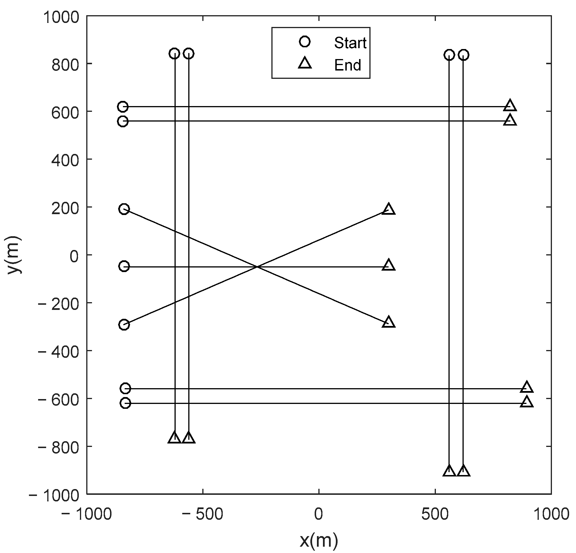
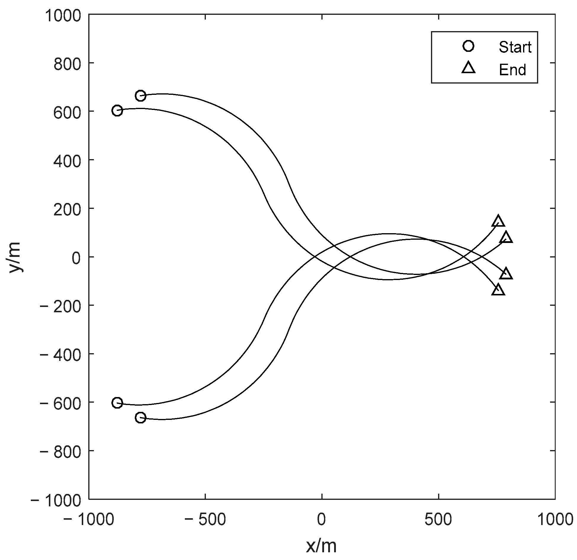
Example 1. 

We consider eleven objects in example 1. The initial states of objects 1, 2, 3, 4, 5, 6, 7, 8, 9, 10 and 11 are ${[-860,17,620,0]}^T$, ${[-860,17,560,0]}^T$, ${[-620,0,860,-17]}^T$, ${[-560,0,860,-17]}^T$, ${[-860,24,-620,0]}^T$, ${[-860,24,-560,0]}^T$,${[-860,19,200,-8]}^T$,${[-860,19,-50,0]}^T$, ${[-860,19,-300,8]}^T$, ${[620,0,860,-26]}^T$ and ${[560,0,860,-26]}^T$, respectively. They appear at $t=1 \mathrm{s}$, $1 \mathrm{s}$, $4 \mathrm{s}$, $4 \mathrm{s}$, $9 \mathrm{s}$, $9 \mathrm{s}$, $9 \mathrm{s}$, $27 \mathrm{s}$, $27 \mathrm{s}$, $32 \mathrm{s}$ and $32 \mathrm{s}$, respectively, and disappear at $t=100 \mathrm{s}$, $100 \mathrm{s}$, $100 \mathrm{s}$, $100 \mathrm{s}$, $68 \mathrm{s}$, $68 \mathrm{s}$, $68 \mathrm{s}$, $100\mathrm{s}$, $100 \mathrm{s}$, $100\mathrm{s}$ and $100 \mathrm{s}$, respectively. The eleven objects consist of close objects (such as objects 10 and 11, objects 8 and 9, objects 3 and 4, and objects 1 and 2) and crossing objects (such as objects 5, 6 and 7). Objects 5, 6 and 7 cross their paths at $t=39.25 \mathrm{s}$. The true trajectories of the eleven objects is given in Figure 1.

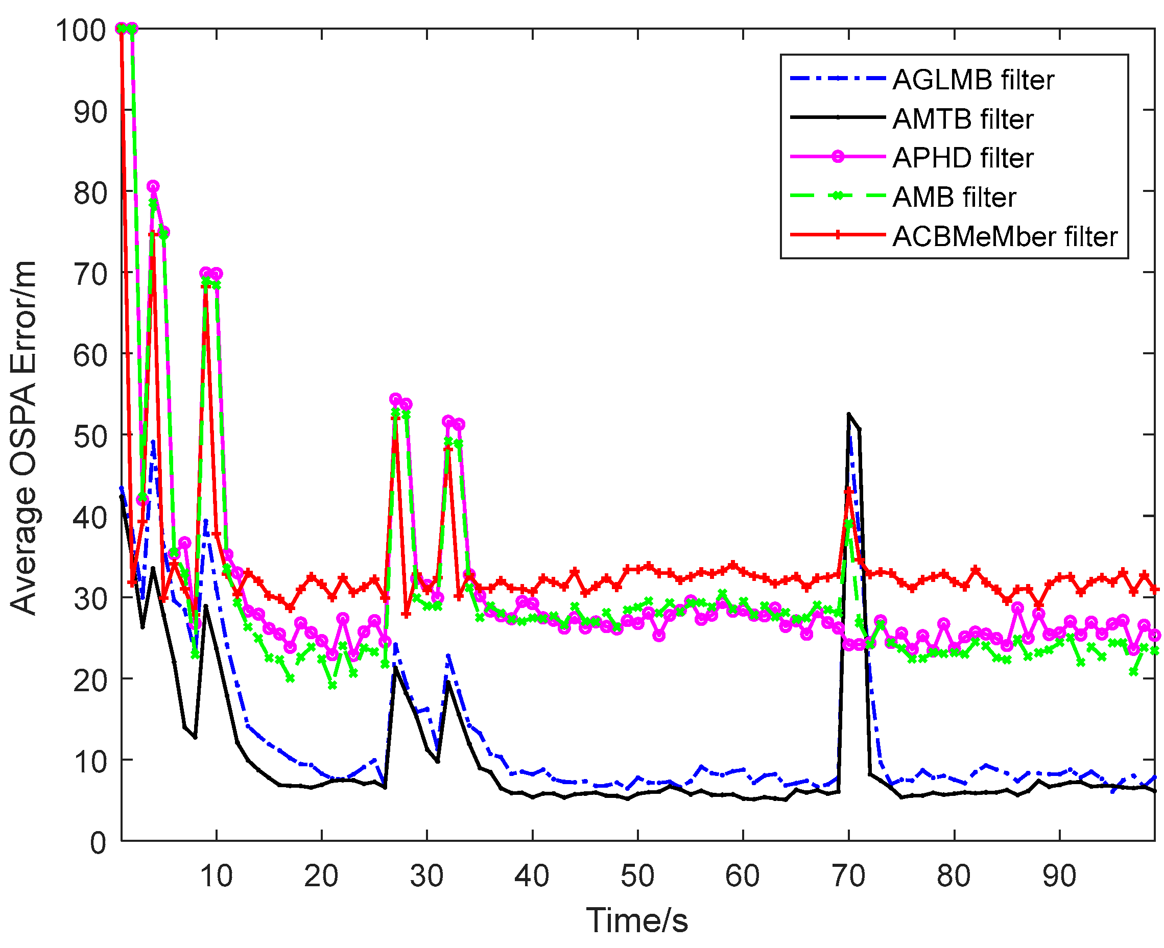
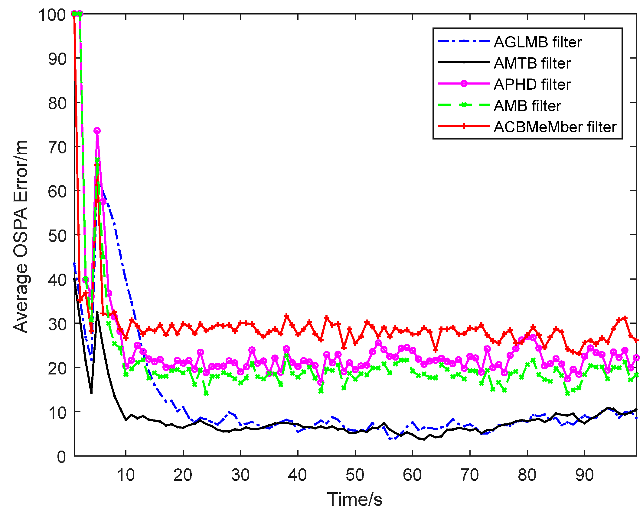
In the experiment, the relevant parameters of the AMTB filter were set to ${\tau }_r=0.005$, $q_a=7.824$, $v_{\max }=50 {\mathrm{ms}}^{-1}$ and $v_{\min }=5 {\mathrm{ms}}^{-1}$. Using the five adaptive filters to handle the simulated measurements for 200 Monte Carlo runs, we obtained their tracking results. According to the OSPA error in Figure 2 and

Table 1. OSPA and OSPA⁽²⁾ errors, cardinality error and performing time in Example 1.

Filter	ACMeMber	AMB	APHD	AGLMB	AMTB
OSPA error (m)	33.8873	30.6815	31.6086	12.8324	10.2323
OSPA(2) error (m)	NA	NA	NA	19.2660	15.4079
Cardinality error	0.3165	0.5113	1.0810	0.1954	0.1696
Performing time (s)	1.2703	0.6614	0.3933	9.0452	0.7310

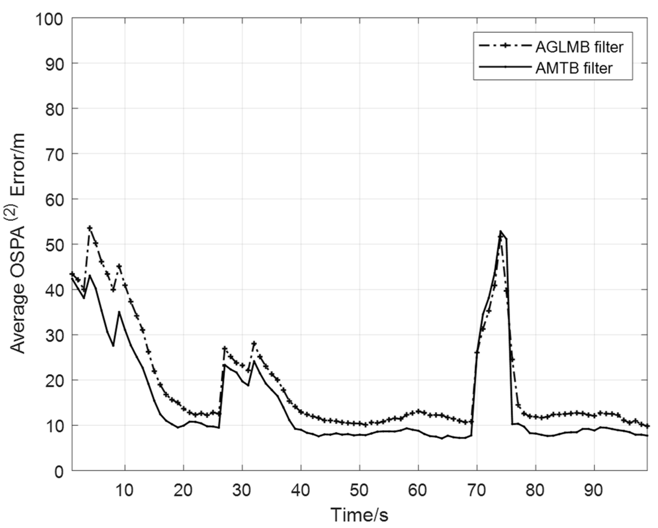
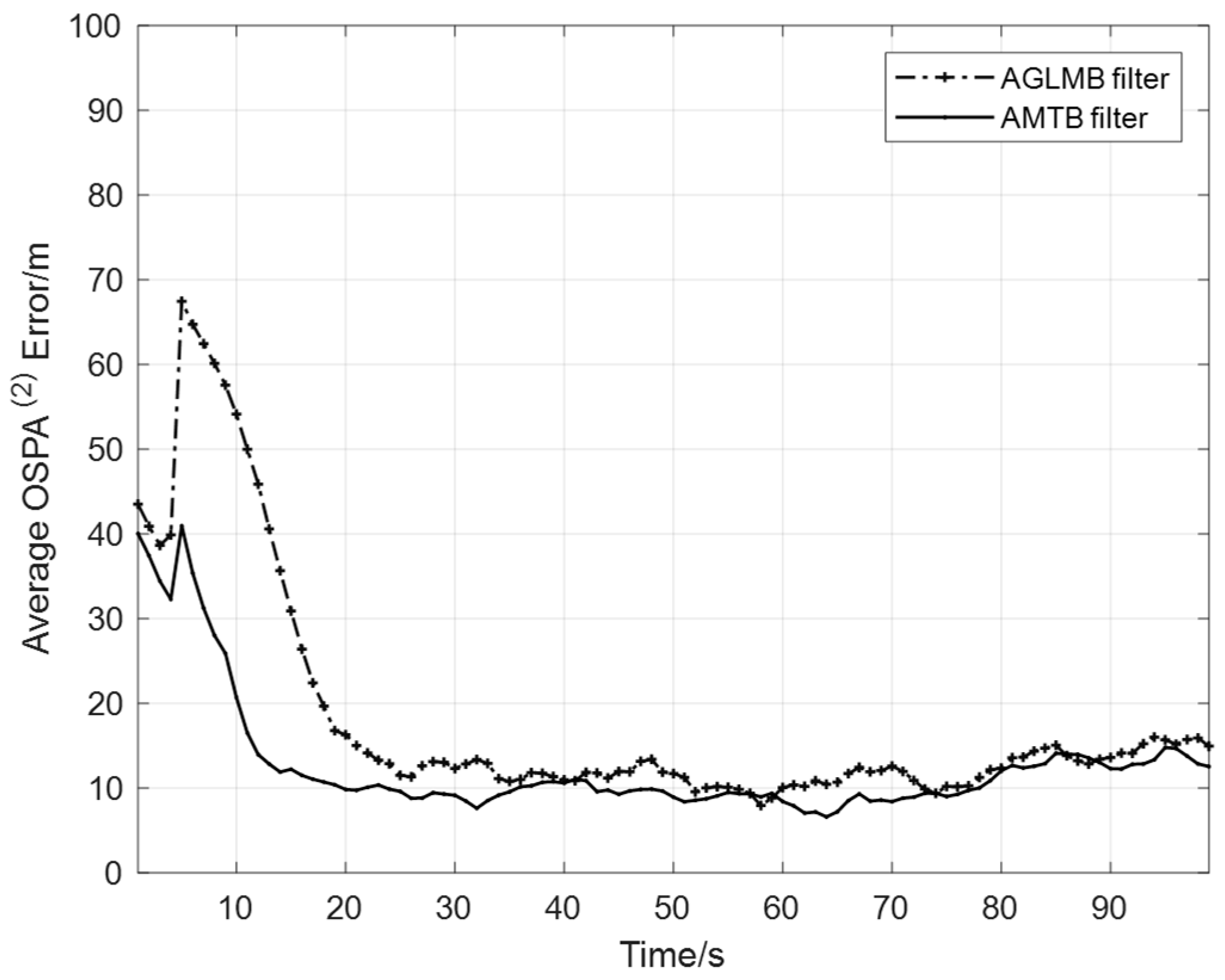
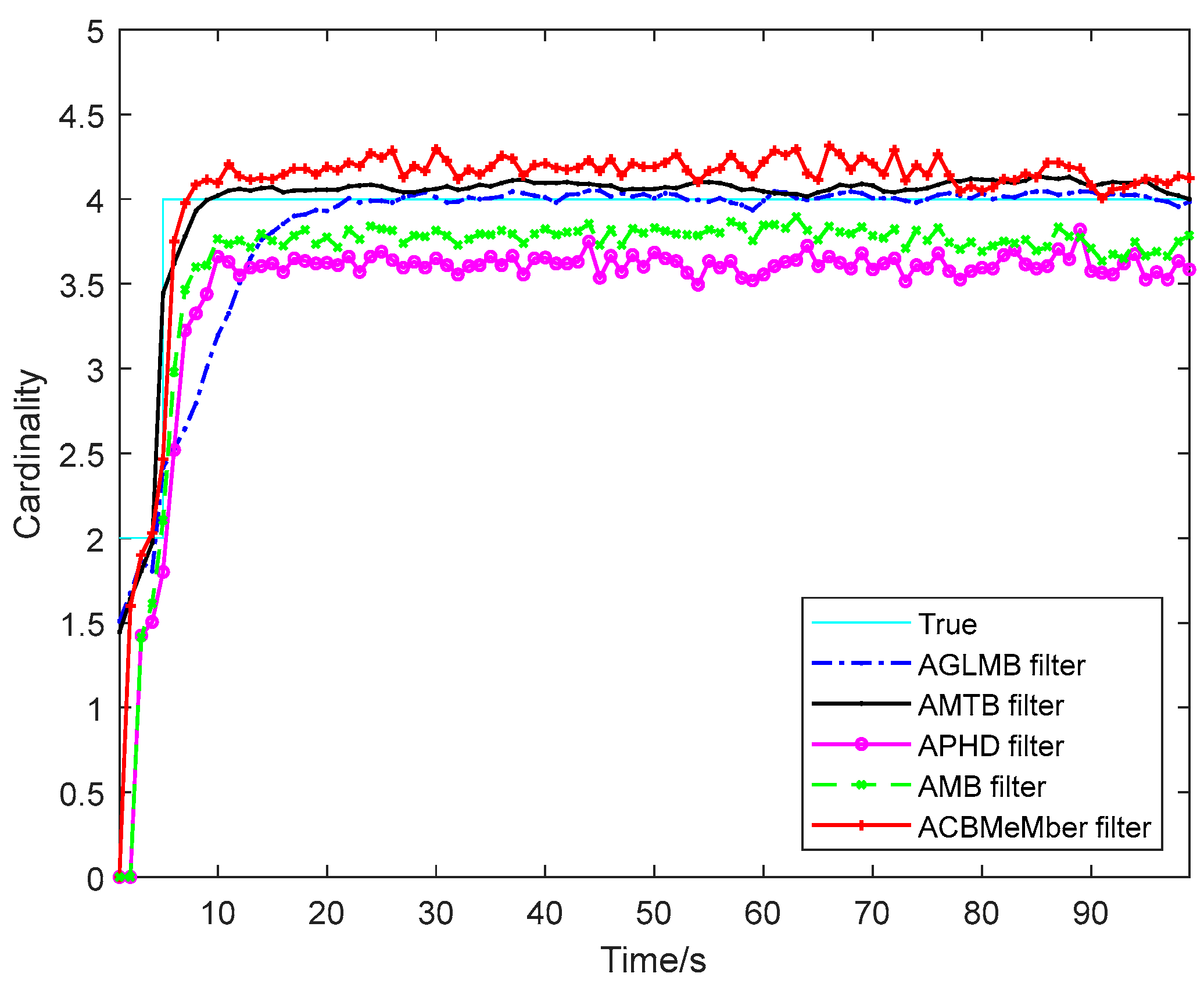
, the ACMeMber filter, AMB filter and APHD are inferior to the AMTB filter and AGLMB filter. This is because the former three filters require a high detecting probability, whereas the latter two filters avoid this requirement. As seen in Table 1 and Figure 2 and Figure 3, the AGLMB filter had larger OSPA and OSPA⁽²⁾ errors than the AMTB filter, which indicates that the AMTB filter performs better than the AGLMB filter although it obviates the requirement for clutter density. 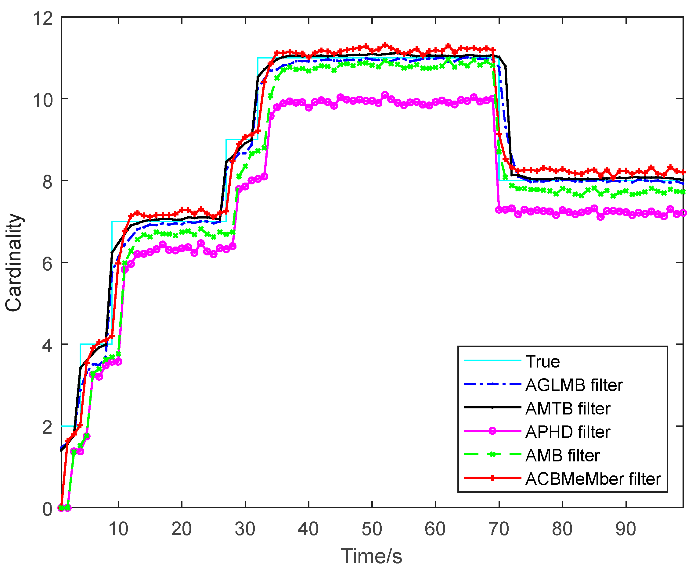The cardinality error in Table 1 and cardinality estimation in Figure 4 reveal that the cardinality error of the AMTB filter is the lowest and its cardinality estimation is the most accurate. As seen in Table 1, the AMTB filter requires significantly less computation time than the AGLMB filter. Several peaks appear in Figure 2 and Figure 3 because of the delayed response of the filter to the object appearing and disappearing.

The experimental results for different noisy standard deviations, different detecting probabilities and different clutter densities over 200 Monte Carlo runs are exhibited in

Table 2. Effect of clutter density on OSPA error at $p_D^{}=0.9$.

${\mathit{N}}_{\mathit{c}}$	ACMeMber	AMB	APHD	AGLMB	AMTB
5	28.8650	29.6414	31.2185	11.1668	8.2281
10	31.2189	29.9661	31.2191	11.2753	8.5712
15	33.8873	30.6815	31.6086	12.8324	10.2323
20	36.0720	31.2233	31.7726	14.0930	12.6169
25	38.0561	31.5900	32.0667	16.7082	16.2992

,

Table 3. Effect of detection probability on OSPA error at $N_c=15$.

${\mathit{p}}_{\mathit{D}}$	ACMeMber	AMB	APHD	AGLMB	AMTB
1.00	12.3744	11.1873	10.9080	5.9300	5.1357
0.95	24.3627	21.6667	22.2138	8.8006	8.0763
0.90	33.8873	30.6815	31.6086	12.8324	10.2323
0.85	38.9061	38.0461	39.1806	13.9446	12.8517
0.80	42.3854	41.9417	45.7909	17.5125	14.9649
0.75	45.3814	45.2975	51.9196	20.7581	18.1959

and

Table 4. Effect of noisy deviation on OSPA error at $p_D^{}=0.9$ and $N_c=15$.

${\mathit{\sigma }}_{\mathit{\alpha }}$ (°)	${\mathit{\sigma }}_{\mathit{r}}$ (m)	ACMeMber	AMB	APHD	AGLMB	AMTB
0.2	2	33.2311	29.6021	30.9143	10.9250	8.5825
0.3	3	33.9630	30.7171	31.6724	13.0685	10.8013
0.4	4	34.4782	31.6870	32.5023	16.2794	13.3886
0.5	5	34.8680	32.2220	32.9217	21.0756	15.7999
0.6	6	35.4487	33.1801	33.9049	26.6639	18.7992
0.7	7	36.1280	33.9897	34.8693	34.5188	21.6057

, which reveal that the AMTB filter had the lowest OSPA error at each pair of noisy standard deviations, each detecting probability and each clutter density. The above fact demonstrates the robustness of the AMTB filter.

Example 2. 

We consider four maneuvering objects. Objects 1, 2, 3 and 4 appear at $t=1 \mathrm{s}$, $1 \mathrm{s}$, $5 \mathrm{s}$ and $5 \mathrm{s}$ and then disappear at $t=100 \mathrm{s}$. Objects 1 and 2 cross their tracks at $t=55.8 \mathrm{s}$ and $t=88.89 \mathrm{s}$, respectively. Objects 3 and 4 cross their tracks at $t=63.92 \mathrm{s}$ and $t=92.75 \mathrm{s}$, respectively. The real trajectories of maneuvering objects is given in Figure 5.

We used the five filters to handle the simulated measurements over 200 Monte Carlo runs. The OSPA and OSPA⁽²⁾ errors and cardinality error in

Table 5. OSPA and OSPA⁽²⁾ errors, cardinality error and performing time in Example 2.

Filter	ACMeMber	AMB	APHD	AGLMB	AMTB
OSPA error (m)	29.3956	21.5289	24.7589	12.2358	8.4621
OSPA(2) error (m)	NA	NA	NA	18.1280	12.6685
Cardinality error	0.2029	0.2976	0.4577	0.1287	0.0908
Performing time (s)	1.0739	0.4489	0.2995	5.0927	0.4370

and Figure 6 and Figure 7 and cardinality in Figure 8 indicate that the AMTB filter performed the best among these five filters. As seen in Table 5, the AMTB filter required significantly less computation time than the AGLMB filter.

5. Conclusions

To track multiple targets in the presence of unknown clutter density, unknown survival probability and unknown initial state and error covariance, we propose an adaptive marginal multi-target Bayes filter without the need for clutter density. This filter delivers the track label, existence probability and PDF of the object. It uses the least squares technique to deal with two consecutive scans of the unused measurements to establish the potential birth target, uses the gating technique to remove the clutter-originated measurements, and uses the 2-dimensional assignment to associate the measurements with the existing targets. In terms of the assignment result, the AMTB filter selects either one of multiple updated PDFs of an existing object or its predicted PDF as its PDF. It establishes newborn targets by using the 2-dimensional assignment to associate the unused measurements with the potential birth targets. A newborn target is established if an unused measurement is assigned to a potential birth target. The simulation results demonstrate that higher tracking accuracy can be acquired by the AMTB filter than by the adaptive RFS-based filters. Its OSPA and OSPA⁽²⁾ errors, and cardinality error were lower than those of the adaptive RFS-based filters. The AMTB filter achieved higher tracking accuracy than the adaptive RFS-based filters, and therefore it has potential applications in real-world multi-target tracking systems, especially in situations where obtaining the clutter density and survival probability is difficult. This article involves the application of the AMTB filter in radar MTT. Further research and real-world testing may help solidify its practical utility in various applications.