Underwater Target Recognition via Cayley-Klein Measure and Shape Prior Information in Hyperspectral Imaging

Abstract

Underwater target detection plays a vital role in various application scenarios, ranging from scientific research to military and industrial operations. In this paper, a detection method via the Cayley–Klein measure and a prior information of shape is proposed for the issue of hyperspectral underwater target identification. Firstly, by analyzing the data features of underwater targets and backgrounds, a background suppression algorithm based on Cayley–Klein measure is developed to enhance the differentiation between underwater targets and backgrounds. Then, a local peak-based algorithm is designed to discriminate potential underwater target points based on the local peak features of underwater targets. Finally, pseudo-target points are eliminated based on the priori shape information of underwater targets. Experiments show that the algorithm proposed is efficient and can effectively detect underwater targets from hyperspectral images.

1. Introduction

Generally, the process of classical method of target detection for hyperspectral remote sensing images can be expressed as follows: the spectral features of the image data points are projected onto a given plane by a certain criterion (i.e., detector) to ensure that the target and the backgrounds are located at different positions in this detection result plane, and then the target is separated from the background by a method of threshold segmentation [1]. During the detection process of hyperspectral targets, different models describing the background lead to different classifications of hyperspectral target detection methods. The classical methods of target detection for hyperspectral remote sensing images are divided into two categories: structured and unstructured backgrounds [2]. Three mathematical models exist to describe the spectral variation of pixels in hyperspectral images for structured background target detection: the probability density model, the subspace model, and the linear spectral hybrid model. Apart from the structured background model, a small number of hybrid detectors that combine the advantages of both have been investigated, and have been developed for both hybrid structured and unstructured detectors. Unlike the structured background method, the unstructured background detectors do not adopt this structured model of endmember signals with corresponding components to express background information. Instead, the background is treated as a statistical model conforming to a multivariate Gaussian distribution, and uniformly models the background and noise as the background. Typical methods include Generalized Likelihood Ratio (GLR), Adaptive Coherence Estimator (ACE), and Adaptive Matching Filter (AMF).

In recent years, several new methods of pattern recognition and machine learning have emerged in the field of hyperspectral remote sensing image target detection, including the Kernel Method [3], Sparse Representation Model [4], Discriminant Subspace Analysis [5,6] and Deep Learning Model [7]. For instance, a hyperspectral image anomaly detection method based on Support Vector Data Description (SVDD) was proposed by Li et al. [8], which can describe the image background depending on a few pixels without requiring the prior knowledge of data distribution. However, the shortcoming of this method mainly lies in the fact that the selection of kernel parameters of the algorithm is too dependent on human experience, and no scientific method of parameter selection is proposed. Wu et al. proposed a Collaborative Representation based Detector (CRD) algorithm for anomaly detection in hyperspectral images [9], assuming that background pixels can be expressed as linear combinations of neighboring pixels, while anomalous pixels do not follow this property, and using this property for anomalous target detection. The algorithm is a non-parametric method that does not require estimation of the background covariance matrix and has a closed solution.

Although algorithms such as deep learning have been progressively applied to hyperspectral target extraction, they also suffer from several bottlenecks: Firstly, the establishment of models in deep learning methods often requires certain numbers of reliable training samples, which is generally not satisfied in the field of hyperspectral target detection since the prior knowledge of hyperspectral target detection problem is only a single target spectrum, and the generalization and migration of the model is poor [10]. Secondly, it also possesses numerous parameters for deep learning methods to determine, and there is not enough data for cross-validation of multiple parameters in hyperspectral target detection [11]. Lastly, the computational complexity of machine learning methods tends to increase dramatically along with the expansion of problem scale, and the sample sets in hyperspectral target detection often reach megapixels, making it difficult to meet the requirements in real-time.

The above analysis shows that the existing hyperspectral target detection algorithms are mainly oriented to land domain scenarios, and there are few research cases for underwater target detection. Underwater target detection is a very interesting problem: many authors have proved that hyperspectral imagery could enable to retrieve efficiently bathymetry, coral reefs and sea grass [12,13,14,15]. However, only a few ones have dealt with the detection problem in such a context. For example, in [16], the purpose of the authors is more to classify pixels rather than to detect spared target pixels among the background. Most similarity criteria of hyperspectral pixels consider a single spectral dimension, and multi-source information including global, local, spectral, shape and other information is less comprehensive consideration. Afterward, it is difficult for the existing hyperspectral target detection algorithms to strike a balance between efficiency and accuracy, and further research is still required to improve the detection efficiency while meeting the accuracy requirements.

In this paper, we try to present a new method of detecting underwater targets in hyperspectral imaging, which not only guarantees the detection probability but also considers the efficiency. The development of the new algorithm is based on the hyperspectral images of underwater targets acquired by an unmanned airborne hyperspectral camera.

2. Study Area and Data

The hyperspectral remote sensing monitor employed in this experiment is the HY-9010-U unmanned aerial vehicle (UAV)-mounted hyperspectral imaging equipment, which was developed and produced by Hangzhou Spectral Imaging Technology Co., Ltd. (Hangzhou, China), as shown in Figure 1a, the details can be seen in

Table 1. Parameters of the HY-9010-U UAV -mounted hyperspectral imaging instrument.

Imaging Mode	Dispersive Push-Broom Mode
Spectral range	400–1000 nm
Spectral resolution	2.8 nm
Spatial resolution	7 cm
Number of spatial pixels	1920 (1×), 480 (4×)
Number of spectral bands	1200 (1×), 300 (4×)
Slit	25 μm
Relative aperture	F2.6
Output pixel bit depth	12 bits
Maximum frame rate (full spectrum acquisition)	128 fps
Lens focal length	12.5 mm/35 mm interchangeable.
Height of UAV	100 m

. The site of data collection is near the coast of Yantai, with favorable aquatic conditions. The seawater in this area is 1–20 m in depth, crystal-clear, and free from various obstructions such as high-rise buildings. Also, the flat terrain along the coast is conducive to taking off and landing of the UAV. During the experiment, the weather was sunny, and the lighting conditions were good, ranging from 700 to 895 lux, which was conducive to the collection of hyperspectral images by the unmanned aerial vehicle. The data were collected on 9 October 2022, by deploying the UAV that mounted with a hyperspectral camera to perform aerial detection of the sea surface, the unmanned underwater vehicle (UUV) (Figure 1b) was used as the underwater loading platform, and the acquired hyperspectral data of underwater targets are shown in Figure 1c. The experimental area is an aquaculture zone where suspended particles in the water can reduce light penetration and may have an adverse effect on the experiment.

The UUV shown in Figure 1b is approximately 50 cm in length and 50 cm in width. As can be seen from Figure 1c, the channels of R, G, and B correspond to the 111th, 60th, and 32nd bands, respectively. The red area is the real reference of the UUV on the ground. To evaluate the impact of the UUV on target detection performance at different water depths, the hyperspectral dataset at four different water depths: 0.1 m, 1.5 m, 3.0 m, and 5 m were collected in this study. The number of samples at different depths is listed in

Table 2. The number of the underwater target at different depths.

Depth of the Target	Number of the Samples
0.1 m	65
1.5 m	23
3 m	17
5 m	53

. Light waves of different wavelengths are absorbed to varying degrees when penetrating water, showing a significant variation in the intensity of absorption. Since there is a valley in the absorption spectrum of water at 300 nm to 900 nm, it is favorable for light waves of this wave band to penetrate water, while those of other wave bands cannot penetrate due to the absorption by water.

3. Method of Recognition

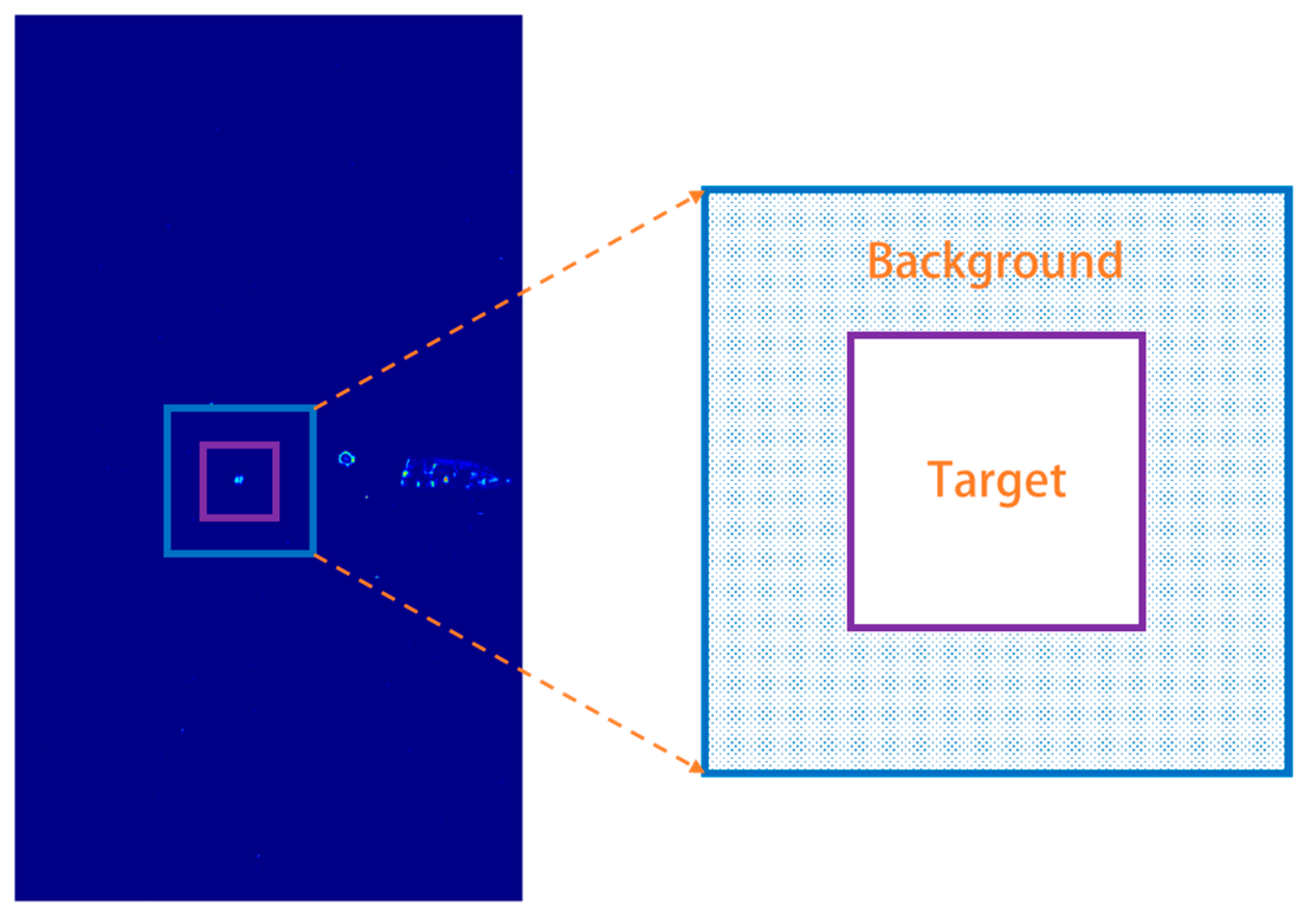
3.1. Hyperspectral Background Field Suppression Based on Cayley–Klein Measure

Let $\mathrm{I}\in {\mathrm{R}}^{{\mathrm{d}}_1\times {\mathrm{d}}_2\times {\mathrm{d}}_3}$ be a hyperspectral image, where $\mathrm{I}$ refers to the original data, while ${\mathrm{d}}_1$, ${\mathrm{d}}_2$, and ${\mathrm{d}}_3$ represent the height, width, and number of spectral bands of the hyperspectral image, respectively. Let $\mathrm{x}\in {\mathrm{R}}^{{\mathrm{d}}_3}$ be the spectral vector corresponding to each pixel. A number ($\mathrm{N}$) of samples are randomly selected from the original hyperspectral image to comprise a dataset of $\left\{{\mathrm{x}}^{\mathrm{k}}\right\}\subset \mathrm{I}$, where $\mathrm{k}=\mathrm{1,2},\dots ,\mathrm{N}$. Let $\mathrm{m}$ and $\sum$ represent the mean and covariance matrix of the dataset, respectively. In this study, given the extremely small proportion of the target of the UUV in the entire image, it can be approximated that $\left\{{\mathrm{x}}^{\mathrm{k}}\right\}$ represents the background field dataset. To calculate the discriminability of any spectral vector and the background field, the Mahalanobis distance is taken as a measure of similarity [17]. The Mahalanobis distance is expressed as follows:

$$d_M\left({\mathsf{x}}_o,{\mathsf{x}}_p\right)={\left({\mathsf{x}}_o-{\mathsf{x}}_p\right)}^T\sum \left({\mathsf{x}}_o+{\mathsf{x}}_p\right)$$

(1)

where ${\mathrm{d}}_{\mathrm{M}}$ represents the Mahalanobis distance measure, ${\mathrm{x}}_{\mathrm{o}}$ and ${\mathrm{x}}_{\mathrm{p}}$ are referred to as the two spectral vectors, and T denotes the transpose. The Mahalanobis distance plays a role in mitigating the impact of the background field, enhancing the discriminability between the target and the background field, and improving the accuracy of target detection. In addition, the Mahalanobis distance can be used to transform the high-dimensional space in an image into a low-dimensional space, thus improving the efficiency of data processing. The calculation of the Mahalanobis distance requires the inversion of the covariance matrix, which is in essence a linear measure. However, hyperspectral image data usually have high dimensionality, and the estimated covariance matrix is ill-conditioned in high-dimensional space, thus making its inversion unstable or impractical. Previous studies show that the Cayley–Klein metric matrix is capable to approximate the Mahalanobis distance in extreme cases [18]. Thus, this study introduces the Cayley–Klein measure to define the pixel similarity of the hyperspectral image. In order to obtain the Cayley–Klein measure, $\mathrm{m}$ and $\sum$ are used in this study to define two invertible symmetric matrices ${\mathrm{G}}^{\pm }$ as follows:

$${\mathit{G}}^{\pm }=\left(\begin{array}{cc}\sum & -\sum \mathit{m}\\ -{\mathit{m}}^T\sum & {\mathit{m}}^T\sum \mathit{m}\pm k^2\end{array}\right)\left(k>0\right)$$

(2)

where ${\mathrm{G}}^{+}$ and ${\mathrm{G}}^{-}$ denote positive definite matrix and positive indefinite matrix, respectively. The bilinear form of ${\mathrm{G}}^{\pm }$ is expressed as follows:

$${\sigma }^{\pm }\left({\mathit{x}}_o,{\mathit{x}}_p\right)=\left({\mathit{x}}_o^T,1\right){\mathit{G}}^{\pm }\left(\begin{array}{c}{\mathit{x}}_p\\ 1\end{array}\right)={\left({\mathit{x}}_o-\mathit{m}\right)}^T\sum \left({\mathit{x}}_p-\mathit{m}\right)\pm k^2\left(k>0\right)$$

(3)

According to Equation (3), Cayley–Klein measures can be combined such as ${\mathrm{d}}_{\mathrm{E}}({\mathsf{x}}_{\mathrm{o}},{\mathsf{x}}_{\mathrm{p}})$, ${\mathrm{d}}_{\mathrm{H}}({\mathsf{x}}_{\mathrm{o}},{\mathsf{x}}_{\mathrm{p}})$:

$$d_E\left({\mathsf{x}}_o,{\mathsf{x}}_p\right)=\frac{k}{2i}\log \left(\frac{{\sigma }_{{\mathsf{x}}_o{\mathsf{x}}_p}^{+}+\sqrt{{\sigma }_{{\mathsf{x}}_o{\mathsf{x}}_p}^{+2}-{\sigma }_{{\mathsf{x}}_o{\mathsf{x}}_o}^{+}\cdot {\sigma }_{{\mathsf{x}}_p{\mathsf{x}}_p}^{+}}}{{\sigma }_{{\mathsf{x}}_o{\mathsf{x}}_p}^{+}-\sqrt{{\sigma }_{{\mathsf{x}}_o{\mathsf{x}}_p}^{+2}-{\sigma }_{{\mathsf{x}}_o{\mathsf{x}}_o}^{+}\cdot {\sigma }_{{\mathsf{x}}_p{\mathsf{x}}_p}^{+}}}\right)$$

(4)

$$d_H\left(x_o,x_p\right)=-\frac{k}{2}\log \left(\frac{{\sigma }_{{\mathsf{x}}_o{\mathsf{x}}_p}^{-}+\sqrt{{\sigma }_{{\mathsf{x}}_o{\mathsf{x}}_p}^{-2}-{\sigma }_{{\mathsf{x}}_o{\mathsf{x}}_o}^{-}\cdot {\sigma }_{{\mathsf{x}}_p{\mathsf{x}}_p}^{-}}}{{\sigma }_{{\mathsf{x}}_o{\mathsf{x}}_p}^{-}-\sqrt{{\sigma }_{{\mathsf{x}}_o{\mathsf{x}}_p}^{-2}-{\sigma }_{{\mathsf{x}}_o{\mathsf{x}}_o}^{-}\cdot {\sigma }_{{\mathsf{x}}_p{\mathsf{x}}_p}^{-}}}\right)$$

(5)

According to experimental experience, ${\mathrm{d}}_{\mathrm{E}}({\mathbf{x}}_{\mathrm{o}},{\mathbf{x}}_{\mathrm{p}})$ is conducive to the processing of hyperspectral image and the Cayley–Klein measure is selected with the value of $\mathrm{k}$ being set to 0.5. For the subsequent judgment of the underwater target, it is necessary to take the neighboring pixels around a certain pixel for similarity discrimination. At this time, $\mathrm{m}$ and $\sum$ can be obtained by using the local pixel set. To make use of both global and local information simultaneously, a new measure of ${\mathrm{d}}_{\mathrm{F}}\left({\mathbf{x}}_{\mathrm{o}},{\mathbf{x}}_{\mathrm{p}}\right)$ is proposed as follows:

$$d_F\left(x_o,x_p\right)=\frac{1}{\sqrt{d_E^{global}\left({\mathsf{x}}_o,{\mathsf{x}}_p\right)\cdot d_E^{local}\left({\mathsf{x}}_o,{\mathsf{x}}_p\right)}}$$

(6)

In Equation (6), ${\mathrm{d}}_{\mathrm{E}}^{\mathrm{g}\mathrm{l}\mathrm{o}\mathrm{b}\mathrm{a}\mathrm{l}}\left({\mathbf{x}}_{\mathrm{o}},{\mathbf{x}}_{\mathrm{p}}\right)$ and ${\mathrm{d}}_{\mathrm{E}}^{\mathrm{l}\mathrm{o}\mathrm{c}\mathrm{a}\mathrm{l}}\left({\mathbf{x}}_{\mathrm{o}},{\mathbf{x}}_{\mathrm{p}}\right)$ represent the Cayley–Klein measures created by using the global and local sample sets, respectively. Global sample set are randomly selected in the whole hypespectral image, while local sample set are randomly selected within the local area of the target pixel. For more information, we recommend the reader to [19,20].

Figure 2 shows the comparative results of the three measures, and it can be found out that ${\mathrm{d}}_{\mathrm{E}}^{\mathrm{g}\mathrm{l}\mathrm{o}\mathrm{b}\mathrm{a}\mathrm{l}}$ performs better than ${\mathrm{d}}_{\mathrm{E}}^{\mathrm{l}\mathrm{o}\mathrm{c}\mathrm{a}\mathrm{l}}$ in discriminating the target from the background. Compared with ${\mathrm{d}}_{\mathrm{E}}^{\mathrm{g}\mathrm{l}\mathrm{o}\mathrm{b}\mathrm{a}\mathrm{l}}$ and ${\mathrm{d}}_{\mathrm{E}}^{\mathrm{l}\mathrm{o}\mathrm{c}\mathrm{a}\mathrm{l}}$, ${\mathrm{d}}_{\mathrm{F}}$ shows greater homogeneity in the target area, while maintaining the discrimination between the target and background. This results in a good balance between inter-class and intra-class dispersion.

To address the impact of random sampling on the algorithm, the sampling process was repeated multiple times, with the average of the Cayley–Klein measure as the final result.

3.2. Local Peak Detection Algorithm for Target Points

Underwater robots and water bodies exhibit different features in hyperspectral imaging, which means local peaks appear in some particular regions. Allowing for this, a local peak detection algorithm is applied to screen out the pixels that may belong to the underwater autonomous vehicle. Let $\mathrm{C}\in {\mathrm{R}}^{{\mathrm{d}}_1\times {\mathrm{d}}_2\times 1}$ be the Cayley–Klein measurement matrix corresponding to the hyperspectral image $\mathrm{I}\in {\mathrm{R}}^{{\mathrm{d}}_1\times {\mathrm{d}}_2\times {\mathrm{d}}_3}$. For any point of $\left(\mathrm{x},\mathrm{y}\right)$ in the measurement matrix, the measurement of $\mathrm{C}\left(\mathrm{x},\mathrm{y}\right)$ can be decomposed into:

$$C\left(x,y\right)=c_t\left(x,y\right)+c_b\left(x,y\right)+\epsilon \left(x,y\right)$$

(7)

where ${\mathrm{c}}_{\mathrm{t}}$, ${\mathrm{c}}_{\mathrm{b}}$, and $\mathsf{\epsilon }$ represent the target component, background component and noise, respectively. Assuming that there is a spectral difference between the UUV and the water, and there is supposed to be a local peak in the corresponding Cayley–Klein measurement, which is similar to the features of the point spread function (SPF), as can be described by a two-dimensional Gaussian function. For the local bright spot-shaped targets, the gray values in the locality are expected to show a peak that can be roughly described by a two-dimensional Gaussian distribution. That is, the target component of ${\mathrm{c}}_{\mathrm{t}}(\mathrm{x},\mathrm{y})$ can be approximately expressed as:

$$f_t(x,y)=\left\{\begin{array}{cc}{I}_i\exp \{-\frac{1}{2}\left[\frac{{(x-x_{oi})}^2}{{\partial }_{1i}^2}+ \frac{{(y-y_{oi})}^2}{{\partial }_{2i}^2}\right]\}& ,(x,y)\in {\mathsf{\Omega }}_i\\ 0& ,(x,y)\notin {\mathsf{\Omega }}_i\end{array}\right.$$

(8)

In the above equation, $\left(\mathsf{\Omega }={\mathsf{\Omega }}_1\cup {\mathsf{\Omega }}_2\cup {\mathsf{\Omega }}_3\cup \cdots \cdots \cup {\mathsf{\Omega }}_n\right)$, where ${\mathsf{\Omega }}_i$ represents the $i$-th target area, $\mathrm{n}$ indicates the number of target areas, and ${\mathrm{I}}_{\mathrm{i}}$ denotes the Cayley–Klein measurement of the $\mathrm{i}$-th target. For those small targets, their small size can be expressed as any $\mathsf{\Delta }{\mathrm{x}}^2+\mathsf{\Delta }{\mathrm{y}}^2={\mathrm{w}}^2$, satisfying $\left({\mathrm{x}}_{\mathrm{o}\mathrm{i}}+\mathsf{\Delta }\mathrm{x},{\mathrm{y}}_{\mathrm{o}\mathrm{i}}+\mathsf{\Delta }\mathrm{y}\right)\notin {\mathsf{\Omega }}_{\mathrm{i}}$, where $\mathrm{w}$ represents a slightly larger value than the target size. By taken account into Equation (6), it can be known that:

$$\begin{array}{c}F(x_{ai},y_{ai})-F(x_{ai}+\mathsf{\Delta }x,y_{ai}+\mathsf{\Delta }y)=\\ \begin{array}{l}\begin{array}{l}{f}_{\mathrm{t}}(x_{oi},y_{oi})+\left[f_{\mathrm{b}}(x_{oi},y_{oi})-f_{\mathrm{b}}(x_{oi}+ \mathsf{\Delta }x,y_{oi}+\mathsf{\Delta }y)\right]+\\ \left[n(x_{oi},y_{oi})-n(x_{oi}+ \mathsf{\Delta }x,y_{oi}+\mathsf{\Delta }y)\right],\mathsf{\Delta }{x}^2+\mathsf{\Delta }{y}^2=w^2\end{array}\hfill \end{array}\end{array}$$

(9)

When the background changes at a relatively slow pace and the intensity of the noise is much lower than that of the target, the last two terms on the right-hand side of Equation (7) can be ignored, which means:

$$F(x_{ai},y_{ai})-F(x_{ai}+\mathsf{\Delta }x\cdot y_{ai}+\mathsf{\Delta }y)=f_{\mathrm{t}}(x_{oi},y_{oi})=I_i$$

(10)

Notably, the intensity level of noise must be lower compared with the target to satisfy the requirements of Equation (8). In case of salt-and-pepper noise, additional processing is required to apply the equation, which will be explained later.

The target must have a certain intensity, that is, ${\mathrm{I}}_{\mathrm{i}}>\mathrm{T}$, where T indicates a fixed threshold value. Therefore, the discriminant formula used for the selection of the peak features is expressed as:

$$F(x_{oi},y_{oi})-F(x_{oi}+\mathsf{\Delta }x,y_{oi}+\mathsf{\Delta }y)>T$$

(11)

In practice, noise is inevitably present in the Cayley–Klein measures, which causes the frequent deviations of local peaks. To reduce the impact of noise on local peak detection, it is proposed in this paper to denoise the Cayley–Klein measures through median filtering. Figure 3 shows the local peak detection algorithm intended for the target points. It can be seen that there is a local peak of ${\mathrm{d}}_{\mathrm{F}}$ in the target area rather than the background area, and there are multiple ${\mathrm{d}}_{\mathrm{F}}$ peaks in the surrounding areas. On this basis, it is possible to distinguish the target from the background areas.

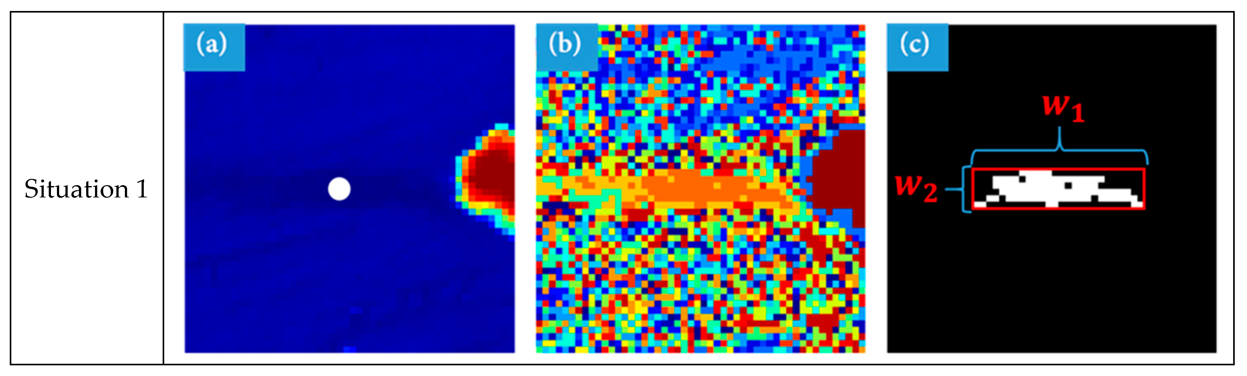
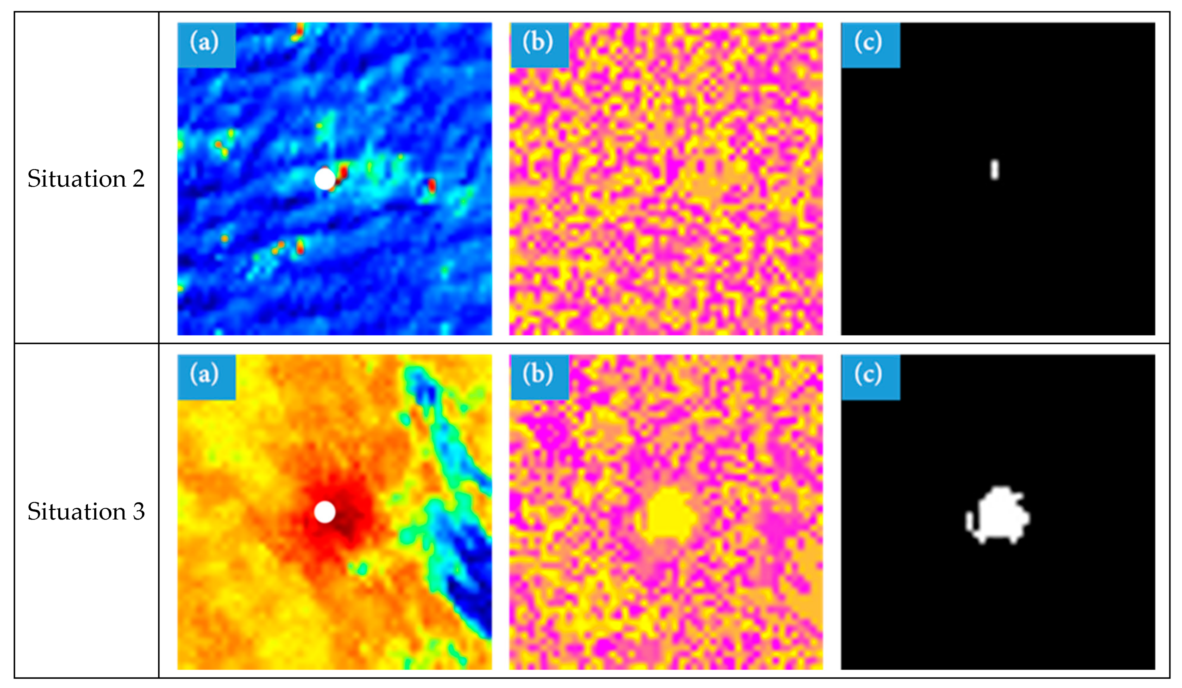
3.3. Pseudo-Target Criterion Based on Shape Prior Information

To distinguish the real underwater targets from the pseudo-targets as previously detected, the prior shape information of underwater targets is used to remove the pseudo-target points that contradict the prior shape information. The homogeneous region at any point is extracted from the local region of ${\mathrm{d}}_{\mathrm{F}}$, which can be achieved through methods such as binarization and clustering.

The methods of thresholding and clustering can be used to extract homogenous regions. The thresholding method is simple to operate, but its threshold value is difficult to determine. An improper threshold value will affect the accurate extraction of homogeneous regions, resulting in difficulties in the subsequent shape discrimination. Clustering is a common unsupervised method, which divides a group of objects into several categories, with the core concept of maximizing the inter-class distances while minimizing the intra-class distances [21]. The classical clustering algorithms include: partitioning [22], density [23], graph theory [19], and grid-based method [24]. The K-means [25] is a typical partitioned clustering algorithm, which is only applicable to spherical clustering, and the clustering results are easily affected by the initial clustering center. The density-based noise can be found by using the Density-Based Spatial Clustering of Application with Noise (DBSCAN) [26] algorithm, but the clustering results are easily affected by the threshold and neighborhood radius. Rodriguez et al. [27] proposed the Density Peak Clustering (DPC) algorithm, which believes that the density of the cluster center is higher than that of the surrounding data points and is far away from other high-density points. However, the DPC algorithm only calculates the density according to the distance between data points, which is not suitable for datasets with complex shapes and densities. When distributing data points based on distances, the robustness of the algorithm is poor, and the clustering results are sensitive to the value of the cut-off distance.

The Local Gravitation Model (LGM) [28] is a method for data clustering. It is different from the traditional gravity clustering model, where the modulus length and direction information of the resultant force of the local gravitation are used in the calculation of the local center measure. Considering the efficiency and accuracy of the algorithm, the local gravity gravitation clustering model [29] is used to extract the homogeneous regions from the measurements. The principle of the LGM clustering algorithm is as follows:

Inspired by Newton’s law of universal gravitation, the local gravitation of data points in the clustering process can reflect the relationship between data points and their neighbors. According to the law of universal gravitation, the attraction between two particles can be defined as:

$${\mathit{F}}_{ij}=G\frac{m_i{m}_j}{d_{ij}^2}{\mathit{D}}_{ij}$$

(12)

where ${\mathbf{F}}_{\mathrm{i}\mathrm{j}}$ represents the gravitation between the points of ${\mathrm{X}}_{\mathrm{i}}$ and ${\mathrm{X}}_{\mathrm{j}}$, $\mathrm{G}$ represents the coefficient of gravitation, $\mathrm{m}$ represents the mass of the point ${\mathrm{X}}_{\mathrm{i}}$, ${\mathrm{d}}_{\mathrm{i}\mathrm{j}}$ represents the distance between the points of ${\mathrm{X}}_{\mathrm{i}}$ and ${\mathrm{X}}_{\mathrm{j}}$, the unit vector ${\mathbf{D}}_{\mathrm{i}\mathrm{j}}$ is the direction of the line between the two points. Since the gravitation in the local neighborhood is calculated, there is no significant difference in the distance between the data points and the neighbors, so Equation (12) can be simplified as

$${\mathit{F}}_{ij}=G{m}_i{m}_j{\mathit{D}}_{ij}$$

(13)

The Local Resultant Force (LRF) on ${\mathrm{X}}_{\mathrm{i}}$ produced by its $\mathrm{k}$ nearest neighbor points can be simplified as:

$$\mathit{L}\mathit{R}\mathit{F}\left(i,k\right)={\displaystyle \sum }_{j=1}^k{\mathit{F}}_{ij}=G{m}_i{\displaystyle \sum }_{j=1}^k{m}_j{\mathit{D}}_{ij}$$

(14)

where $\mathrm{k}$ represents the number of the nearest neighbor points of ${\mathrm{X}}_{\mathrm{i}}$. According to Equation (14), the greater the mass of ${\mathrm{X}}_{\mathrm{i}}$, the greater the influence on the neighborhood. Similarly, the smaller the mass, the more susceptible it is to the influence of the nearest neighbor points. Therefore, the LRF can be simplified as:

$$\begin{array}{c}\mathit{L}\mathit{R}\mathit{F}\left(i,k\right)=\frac{1}{m_i}{\displaystyle \sum _{j=1}^k}{\mathit{D}}_{ij}\\ \mathrm{s}.\mathrm{t}.m_i=1/{\displaystyle \sum _{j=1}^k}{d}_{ij}\end{array}$$

(15)

On the basis of the above equations, the LGM clustering process includes the following: Firstly, the concentration of the data points is calculated using the LGM model, and the distance between each data point and the points with high concentration is determined based on the concentration. Secondly, the data points with high concentration and high distance values are selected as the clustering centers. Finally, the rest of the data points are allocated based on the principle that the concentration of the points inside the cluster is much higher than that of the boundary points, and the parameters are automatically adjusted by balancing the K-Nearest Neighbor.

The area of the homogeneous region at a point is denoted as ${\mathrm{A}}_{\mathrm{i}}$, which is supposed to satisfy the following conditions:

$$T_A^1<A_i<T_A^2$$

(16)

where ${\mathrm{T}}_{\mathrm{A}}^1$ and ${\mathrm{T}}_{\mathrm{A}}^2$ represent the lower and upper limits of the area threshold, respectively. Given a homogeneous region, the length of ${\mathrm{w}}_1$ and width of ${\mathrm{w}}_2$ of its minimum bounding rectangle can be obtained. Due to the impact of various factors, there may be some true target areas missing from the homogeneous regions, but the proportion of true extractions is supposed to exceed a certain limit of ${\mathrm{T}}_{\mathrm{h}}$.

$$\frac{A_i}{w_1\times w_2}>T_h$$

(17)

Since the underwater targets, which are treated as the focus of this study are squares, the aspect ratio of the minimum bounding rectangle should be close to 1. However, due to the inability to extract the true target area completely, the threshold ${\mathrm{T}}_{\mathrm{l}}$ of the aspect ratio can be appropriately relaxed.

$$\frac{w_1}{w_2}<T_l$$

(18)

Based on the prior experience, the value of ${\mathrm{T}}_{\mathrm{A}}^1$ and ${\mathrm{T}}_{\mathrm{A}}^2$ are set to 30 and 200, respectively; ${\mathrm{T}}_{\mathrm{h}}$ and ${\mathrm{T}}_{\mathrm{l}}$ are set to 0.4 and 1.6, respectively. When the conditions as set out in Equations (16)–(18) are not satisfied in the homogeneous region at a point, this point is treated as a pseudo-target point. The threshold values depend on the spatial resolution of the hyperspectral image. To make the threshold more applicable, we can apply the spatial resolution of the image used in this study as a reference, and the ratio of the resolution of new images to the reference image resolution can be used as a scaling factor for the threshold.

Figure 4 lists the shape information of the candidate target points in the three situations: Situation 1 indicates that although the area of the homogeneous region of the candidate target point meets the requirements of Equation (16), its aspect ratio is higher than ${\mathrm{T}}_{\mathrm{l}}$, indicating that the candidate point is more inclined to linear features (such as cables), which is not consistent with the shape of the underwater target in our work. Situation 2 indicates that the homogeneous area of the candidate target point is smaller than the lower limit ${\mathrm{T}}_{\mathrm{A}}^1$ of the area threshold, indicating that the candidate point tends to be a noise point, which is inconsistent with the area information of the underwater target in this work, and is not a potential underwater target point. Situation 3 indicates that the homogenous region of the candidate target points satisfies Equations (16)–(18), indicating that the candidate points are in good agreement with the shape of the underwater targets in this work, and can be judged as potential underwater target points.

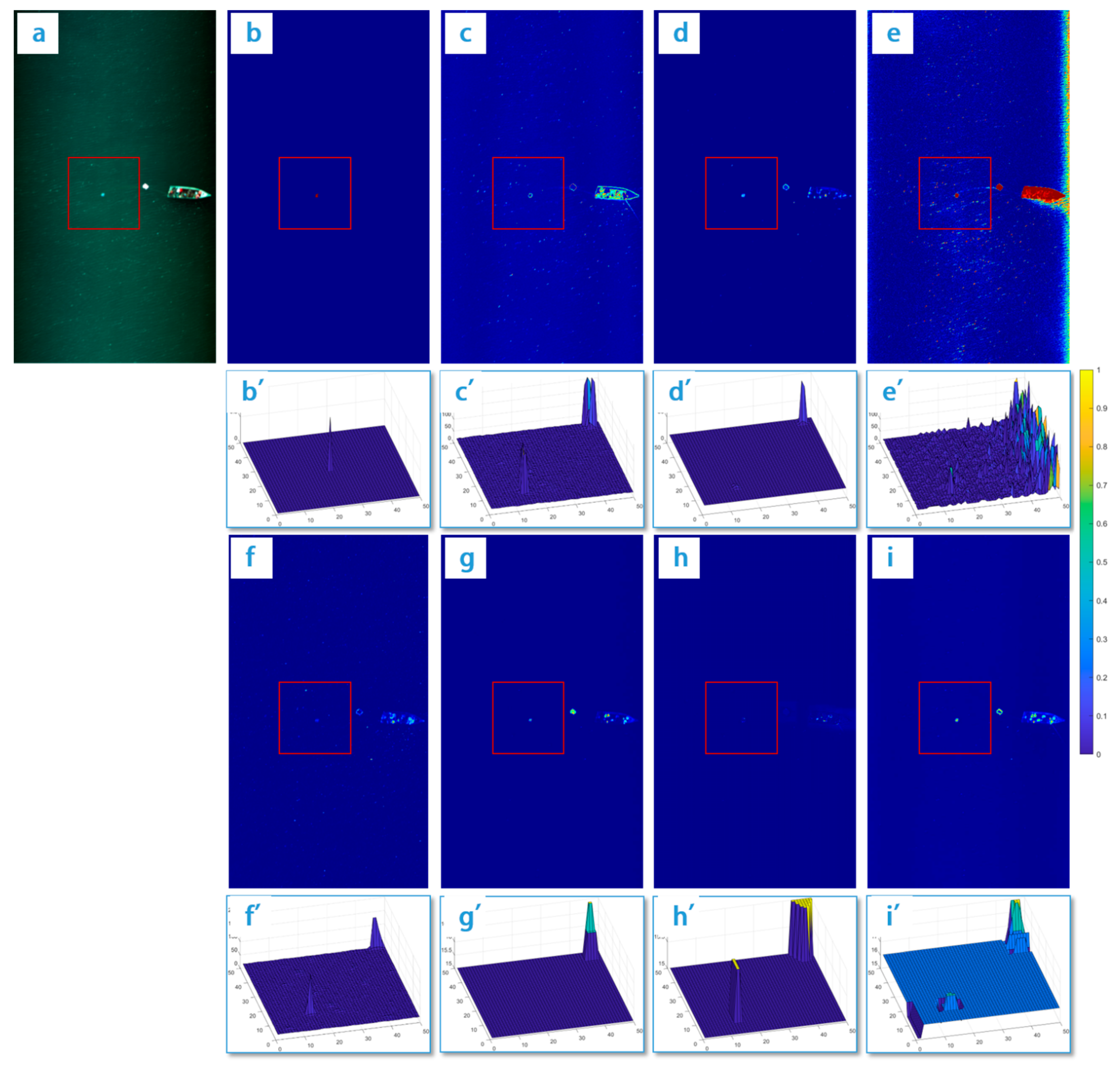
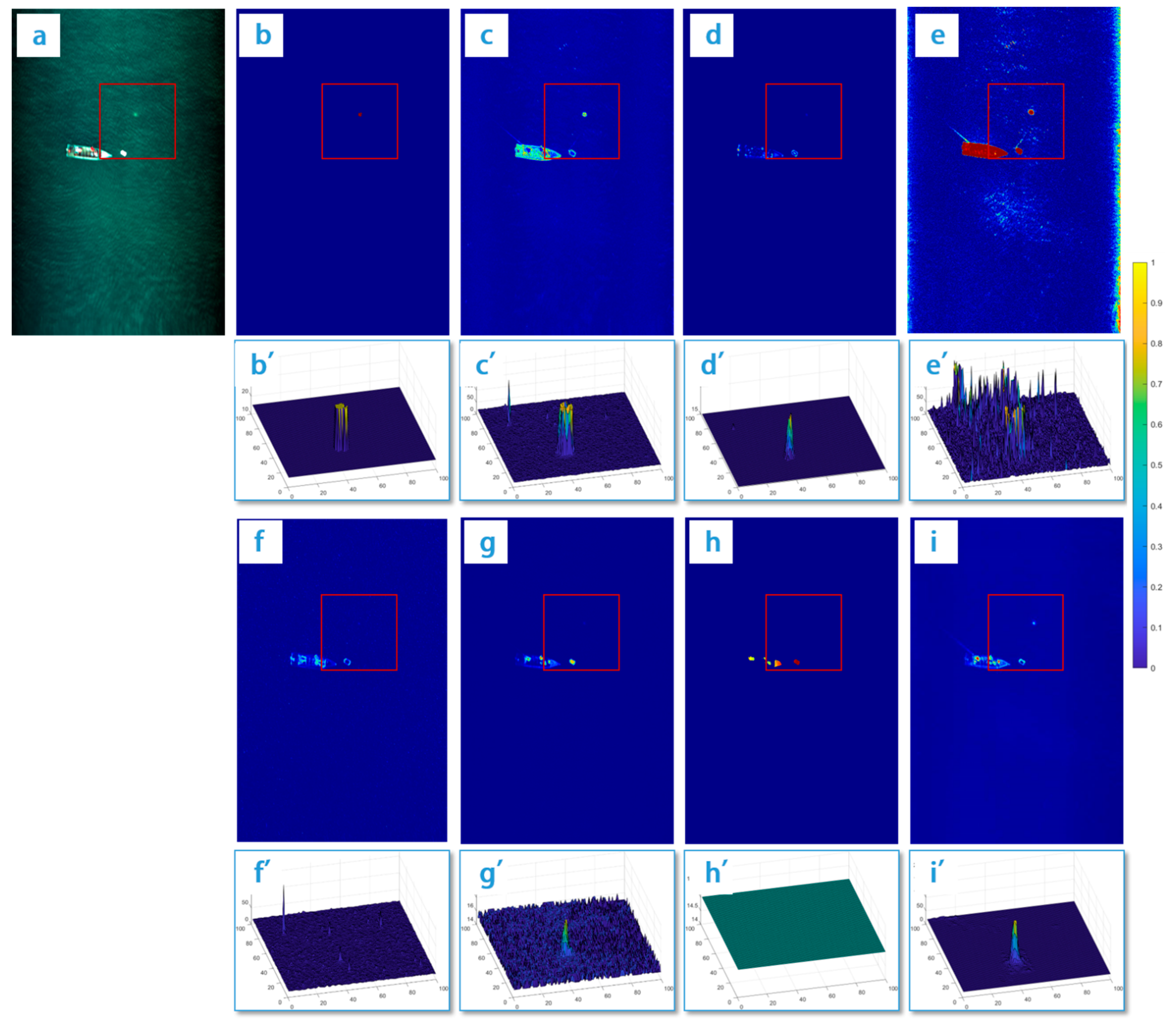
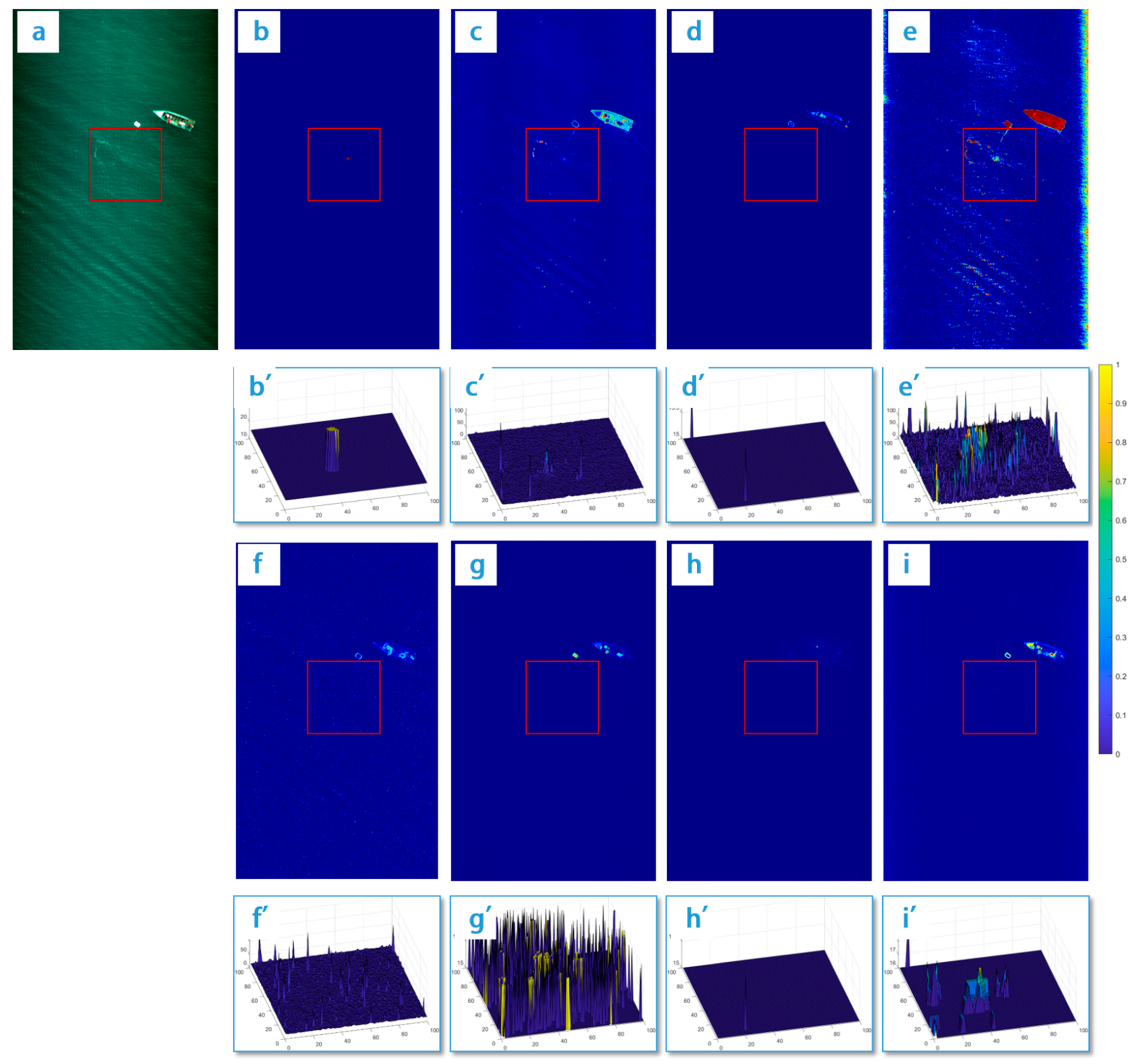
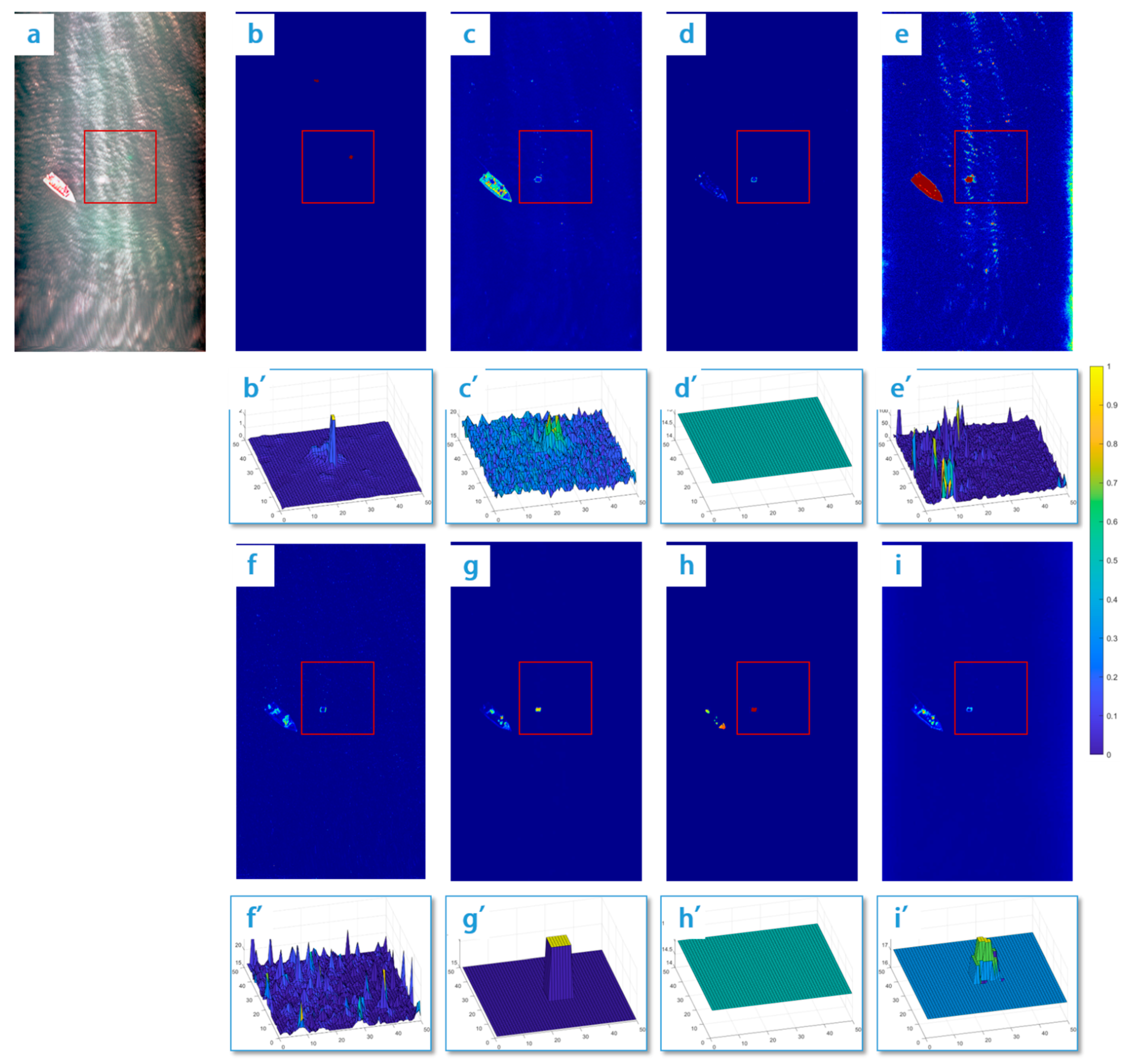
4. Results and Analysis

Considering the particularity of the scene in this work and combining it with the existing literature, existing evaluation indexes are adopted and improved in this work to objectively evaluate the recognition accuracy of underwater targets. TP (True Positive), FP (False Positive), TN (True Negative), and FN (False Negative) are assumed as four indexes calculated from the confusion matrix, which can be used to calculate the False Negatives Rate (FNR) and the False Positive Rate (FPR).

FNR represents the ability of the target detection model to correctly predict the purity of negative samples and reduces the prediction of positive samples as negative samples, that is, the proportion of positive samples predicted as negative samples in the total positive samples. The smaller the FNR value, the better the target detection performance.

$$FNR=\frac{FN}{P}$$

(19)

FPR represents the ability of the target detection model to correctly predict the purity of positive samples, and reduces the prediction of negative samples to positive samples, that is, the proportion of negative samples predicted as positive samples to the total number of negative samples. The smaller the FPR value, the better the target detection performance.

$$FPR=\frac{FP}{N}$$

(20)

The Signal-to-Clutter Ratio (SCR) is defined in Equation (21), where the higher the SCR for the target, the easier it will be detected.

$$SCR=\frac{\left|{\mu }_t-{\mu }_b\right|}{{\sigma }_b}$$

(21)

where ${\mathsf{\mu }}_{\mathrm{t}}$ is the average pixel value of the target, ${\mathsf{\mu }}_{\mathrm{b}}$ and ${\mathsf{\sigma }}_{\mathrm{b}}$ are the average pixel value and the standard deviation value of the pixel value for the adjacent area of the target, respectively.

Since the area of background is much larger than that of target in the research image, the number of the background and the target samples will be unbalanced, (i.e., the positive and negative samples are unbalanced), when all the background areas are used in accuracy evaluation, which reduces the efficiency of evaluating SCR and ROC (Receiver Operating Characteristic). In order to reduce the impact, the target window and background window are set to $20\times 20$ pixels and 4$0\times 40$ pixels, respectively, as shown in Figure 5. The resetting of the calculation area is just for the comparison of the performance of the algorithms.

In general, the FNR and FPR are global indicators, while the improved SCR and ROC in our work belong to local indicators. Therefore, the evaluation system in this work is reasonable by comprehensively evaluating the target detection accuracy from both the global and local areas.

In order to verify the performance and advantages of the proposed algorithms of underwater target detection, seven target detection algorithms for hyperspectral images are compared and analyzed, including Kernel Isolation Forest (KIF) [30], Visual Attention and Background Subtraction (VABS) [31], Sub-Features Grouping and Binary Accumulation (SFBA) [32], Spectral–Spatial Fusion Anomaly Detection Method (SSFAD) [33], Global Reed–Xiaoli (GRX) [34], Local Reed–Xiaoli (LRX) [35] and Low Rank and Sparse Representation (LRASR) [36]. Table 2 shows the comparison results of the precision in different algorithms.

Figure 6, Figure 7, Figure 8 and Figure 9 show the results of experiments 1 to 4, respectively. As can be seen from Figure 9b–i, the background regions of KIF, SFBA and SSFAD are much rougher than those of the algorithms in our work, including VABS, GRX, LRX and LRASA. Figure 6b–i show that the anomalous points detected by some algorithms are located at the central region of the target, while in some other algorithms the points are located at the edge region. For experiment 1, multiple peaks appear in both the target and background regions of SFBA, with the peak values of the target region lower than those in the background region, which leads to the misdetection in experiment 1.

At the same time, with the increase of the depth of the UUV, the background areas of KIF, SFBA and SSFAD become rougher, indicating that the increase in the depth of water will aggravate the mixed pixel phenomenon, which is unfavorable in the target detection. Meanwhile, Figure 9c’,g’ show that the background and target of VABS and LRX become indistinguishable at the water depth of 5 m, indicating a failure in detection efficiency. In addition, the size of the peak value of the target region detected by most algorithms begins to weaken with the increase of water depth, indicating that the distinction between the underwater target and water decreases, which is also detrimental to the recognition of underwater targets. The weakening of water depth on target detection performance is also verified in

Table 3. Comparison results of the precision in different algorithms.

Image	Indicators	Proposed Algorithm	Kernel IF	VABS	SFBA	SSFAD	Global RX	SRX_LOCAL	LRASR
#1 Depth: 0.1 m	FNR	0	0	0	1	0	0	0	0
	FPR	0	0.95	0.95	0.99	0.93	0.94	0.94	0.92
	SCR	0.39	5.23	\	0.82	4.06	228.71	26.82	112.52
#2 Depth: 1.5 m	FNR	0	0	0	0	0	0	1	0
	FPR	0	0.96	0.95	0.94	0.94	0.92	0.83	0.99
	SCR	4.95	4.34	12.12	1.13	0.80	2.71	\	9.95
#3 Depth: 3.5 m	FNR	0	0	1	0	1	1	1	1
	FPR	0	0.97	0.95	0.95	0.88	0.95	0.95	0.94
	SCR	3.66	0.10	\	0.12	0.08	0.14	0.47	\
#4 Depth: 5.0 m	FNR	0	0	1	1	1	0	1	1
	FPR	0.5	0.97	1	1	1	0.98	1	1
	SCR	1.59	0.80	\	0.04	0.04	\	\	\

The symbol ‘\’ represents that the standard deviation value of the pixel value of the adjacent area of the target is 0 or does not exist, which leads to the failure of the calculation of SCR.

. For example, when the water depth is 0.1 m, all the algorithms successfully detect underwater targets except SFBA. However, when the water depth is 5 m, the VABS, SFBA, SSFAD, LRX, and LRASR all fail in the underwater target detection. Table 3 also shows that the algorithms proposed in our work achieve the best performance in the comparison of the FNR and FPR, and the SCR is also close to the best performance of similar algorithms, which demonstrates the advantages and strong detection performance of the proposed algorithm.

The test environment created in this work for a comparative analysis of the efficiency achieved by these algorithms is the Intel(R) Xeon(R) processor with a main frequency of 3.60 GHZ and an internal storage of 32 G. The software environment is MATLAB R2019b. To begin with, the computation is repeated five times for each experimental image, with the average time taken for each computation as the final result. As shown in

Table 4. Comparison of processing efficiency between different algorithms.

Experimental Area	Repeated Times	Computational Cost (s)
		Proposed Algorithm	Kernel IF	VABS	SFBA	SSFAD	Global RX	SRX_LOCAL	LRASR
#1 Water depth: 0.1 m	1st	55.11	724.40	88.85	3.26	1404.55	1.88	2421.82	2799.84
	2nd	53.84	726.09	96.75	3.07	1504.59	1.70	2439.65	3099.21
	3rd	32.06	778.06	90.03	3.40	1390.04	1.81	2355.66	2762.05
	4th	50.43	807.57	90.59	3.20	1454.75	1.74	2121.74	2814.04
	5th	40.73	770.78	97.46	3.23	1552.87	2.14	2488.19	3010.86
	Mean value	46.43	761.38	92.74	3.23	1461.36	1.85	2365.41	2897.20
	Variance	9.81	35.75	4.05	0.12	68.19	0.17	144.26	148.65
#2 Water depth: 1.5 m	1st	40.50	615.51	77.93	3.01	1108.57	1.66	2002.57	2520.30
	2nd	36.58	650.14	80.00	2.99	1248.18	1.98	1970.78	2390.84
	3rd	43.65	600.27	65.13	3.09	1149.64	1.96	2112.07	2371.72
	4th	34.13	705.45	65.93	2.99	1335.02	2.20	1815.17	2384.53
	5th	36.49	617.42	76.43	3.07	1168.50	1.98	2045.39	2199.38
	Mean value	38.27	637.76	73.08	3.03	1201.98	1.96	1989.20	2373.35
	Variance	3.78	41.98	7.02	0.05	90.02	0.19	110.75	114.34
#3 Water depth: 3.0 m	1st	82.76	586.69	67.53	3.01	1061.49	1.52	1602.40	2122.90
	2nd	84.46	574.11	61.41	3.02	1098.43	1.43	1607.27	1910.10
	3rd	85.83	543.97	80.64	3.30	970.73	1.67	1656.37	2055.71
	4th	67.14	547.13	71.56	3.15	1020.24	1.85	1559.98	1952.88
	5th	78.78	588.93	76.66	3.01	1034.11	1.48	1599.74	2133.14
	Mean value	79.79	568.17	71.56	3.10	1037.00	1.59	1605.15	2034.95
	Variance	7.55	21.43	7.55	0.13	47.58	0.17	34.30	100.16
#4 Water depth: 5.0 m	1st	91.83	676.29	92.23	3.17	1326.47	1.87	1926.32	2417.60
	2nd	82.01	677.01	101.58	3.10	1294.71	1.87	1834.17	2337.64
	3rd	89.96	656.63	87.33	3.50	1342.93	2.06	1711.87	2447.91
	4th	82.88	673.32	90.10	3.42	1155.07	1.52	1785.97	2020.00
	5th	92.32	668.77	98.83	3.20	1207.06	1.69	1855.56	2504.81
	Mean value	87.80	670.40	94.01	3.28	1265.25	1.80	1822.78	2345.59
	Variance	4.98	8.35	5.99	0.17	80.90	0.21	79.97	191.75

, the algorithm proposed in this work leads to a significant improvement compared with those of Kernel IF, SSFAD, SRX_LOCAL and LRASR, which makes the processing faster. roughly over 16–60 times It is comparable with VABS, but slightly outperformed by SFBA and Global RX. This algorithm can be refined to further improve computational efficiency. As can be seen above, this algorithm improves accuracy on the basis of ensuring efficiency. Compared with other mainstream ones, the algorithm proposed in this work performs better in balancing accuracy and efficiency.

5. Conclusions

In this work, a detection method based on Cayley–Klein measure and a prior shape information is proposed for better reorganization of underwater targets, which leads to satisfactory outcomes in processing the hyperspectral images captured by UAV. Then, both experiments and comparative analysis are conducted to draw the following conclusions.

Firstly, the Mahalanobis distance can mitigate the impact of background on target identification. Meanwhile, the hyperspectral images are mapped from the high-dimensional space to the low-dimensional space, thus improving the efficiency of data processing. However, this distance is effectively a linear mapping, which means it can fail in high-dimensional space. To address the constraint on processing high-dimensional data with the Mahalanobis distance, we propose to use the Cayley–Klein measure to improve efficiency.

Secondly, the Cayley–Klein measure proposed in this study takes full advantage of global and local information to suppress the background, which enhances the discrimination between the target and the background while improving the heterogeneity of the target area. This is conducive to the identification of targets. Compared with traditional algorithms, the algorithm proposed in this work is applicable to detect the targets at a water depth of up to 5 m.

Thirdly, based on the prior shape information of the underwater target, a false target detection algorithm is developed to improve the accuracy of target identification, which reduces the impact of the false positive rate.

Lastly, the proposed algorithm achieves a high computational efficiency that is comparable with other mainstream target detection algorithms, and a good balance is reached between efficiency and accuracy.

There are limitations of the algorithms proposed in this work because only spectral information is used to conduct underwater target detection and given the account of properties of electromagnetic wave transmission in water. Therefore, it is worthwhile to further explore how to make use of the combined information about spectrum, the intensity of light, and polarization. Another research direction would be to research the relationship between the detected water depth of the underwater target and the water quality.

References

1. Zhang, L. Advance and Future Challenges in Hyperspectral Target Detection. Geomat. Inf. Sci. Wuhan Univ. 2014, 39, 1387–1400. [Google Scholar]
2. Nasrabadi, N.M. Hyperspectral target detection: An overview of current and future challenges. IEEE Signal Process. Mag. 2013, 31, 34–44. [Google Scholar] [CrossRef]
3. Kwon, H.; Nasrabadi, N.M. Kernel matched subspace detectors for hyperspectral target detection. IEEE Trans. Pattern Anal. Mach. Intell. 2005, 28, 178–194. [Google Scholar] [CrossRef]
4. Zhu, D.; Du, B.; Zhang, L. Target dictionary construction-based sparse representation hyperspectral target detection methods. IEEE J. Sel. Top. Appl. Earth Obs. Remote Sens. 2019, 12, 1254–1264. [Google Scholar] [CrossRef]
5. Sun, S.; Liu, J.; Sun, S. Hyperspectral Subpixel Target Detection Based on Interaction Subspace Model. Pattern Recognit. 2023, 139, 109464. [Google Scholar] [CrossRef]
6. Zhou, Y.; Chen, P.; Liu, N.; Yin, Q.; Zhang, F. Graph-Embedding Balanced Transfer Subspace Learning for Hyperspectral Cross-Scene Classification. IEEE J. Sel. Top. Appl. Earth Obs. Remote Sens. 2022, 15, 2944–2955. [Google Scholar] [CrossRef]
7. Hu, X.; Xie, C.; Fan, Z.; Duan, Q.; Zhang, D.; Jiang, L.; Wei, X.; Hong, D.; Li, G.; Zeng, X. Hyperspectral anomaly detection using deep learning: A review. Remote Sens. 2022, 14, 1973. [Google Scholar] [CrossRef]
8. Li, K.; Ling, Q.; Qin, Y.; Wang, Y.; Cai, Y.; Lin, Z.; An, W. Spectral-spatial deep support vector data description for hyperspectral anomaly detection. IEEE Trans. Geosci. Remote Sens. 2022, 60, 5522316. [Google Scholar] [CrossRef]
9. Wu, Z.; Su, H.; Tao, X.; Han, L.; Paoletti, M.E.; Haut, J.M.; Plaza, J.; Plaza, A. Hyperspectral anomaly detection with relaxed collaborative representation. IEEE Trans. Geosci. Remote Sens. 2022, 60, 5533417. [Google Scholar] [CrossRef]
10. Zhang, H.-K.; Li, Y.; Jiang, Y.-N. Deep Learning for Hyperspectral Imagery Classification: The State of the Art and Prospects. Acta Autom. Sin. 2018, 44, 961–977. [Google Scholar]
11. Jia, S.; Jiang, S.; Lin, Z.; Li, N.; Xu, M.; Yu, S. A survey: Deep learning for hyperspectral image classification with few labeled samples. Neurocomputing 2021, 448, 179–204. [Google Scholar] [CrossRef]
12. Lee, Z.; Carder, K.; Mobley, C.; Steward, R.; Patch, J. Hyperspectral remote sensing for shallow waters. ii. deriving bottom depths and water properties by optimization. Appl. Opt. 1999, 38, 3831–3843. [Google Scholar] [CrossRef] [Green Version]
13. Adler-Golden, S.; Acharya, P.; Berk, A.; Matthew, M.; Gorodetzky, D. Remote bathymetry of the littoral zone from A VIRIS, LASH and QuickBird imagery. IEEE Trans. Geosci. Remote Sens. 2005, 43, 337–347. [Google Scholar] [CrossRef]
14. Kallio, K.; Kutser, T.; Hannonen, T.; Koponen, S.; Pul-liainen, J.; Vepsäläinen, J.; Pyhälahti, T. Retrieval of water quality from airborne imaging spectrometry of various lake types in different seasons. Sci. Total Environ. 2001, 268, 59–77. [Google Scholar] [CrossRef] [PubMed]
15. Vahtmäe, E.; Kutser, T.; Martin, G.; Kotta, J. Feasibility of hyperspectral remote sensing for mapping benthic macroalgal cover in turbid coastal waters—A baltic sea case study. Remote Sens. Environ. 2008, 101, 342–351. [Google Scholar] [CrossRef]
16. David, G. An Underwater Target Detection Framework for Hyperspectral Imagery. IEEE J. Sel. Top. Appl. Earth Obs. Remote Sens. 2020, 13, 1798–1810. [Google Scholar]
17. De Maesschalck, R.; Jouan-Rimbaud, D.; Massart, D.L. The Mahalanobis distance. Chemomeasures Intell. Lab. Syst. 2000, 50, 1–18. [Google Scholar] [CrossRef]
18. Struve, H.; Struve, R. Projective spaces with Cayley-Klein metrics. J. Geom. 2004, 81, 155–167. [Google Scholar] [CrossRef]
19. Bi, Y.; Fan, B.; Wu, F. Beyond Mahalanobis metric: Cayley-Klein metric learning. In Proceedings of the IEEE Conference on Computer Vision and Pattern Recognition, Boston, MA, USA, 7–12 June 2015; pp. 2339–2347. [Google Scholar]
20. Bi, Y.; Fan, B.; Wu, F. Multiple Cayley-Klein metric learning. PLoS ONE 2017, 12, e0184865. [Google Scholar] [CrossRef] [Green Version]
21. Mika, S.; Ratsch, G.; Weston, J.; Scholkopf, B.; Mullers, K.-R. Fisher discriminant analysis with kernels. Neural Networks for Signal Processing IX. In Proceedings of the 1999 IEEE Signal Processing Society Workshop (Cat. No. 98th8468), Madison, WI, USA, 25 August 1999; pp. 41–48. [Google Scholar]
22. Patibandla, R.S.M.; Veeranjaneyulu, N. A SimRank based ensemble method for resolving challenges of partition clustering methods. J. Sci. Ind. Res. 2022, 79, 323–327. [Google Scholar]
23. Kriegel, H.; Kröger, P.; Sander, J.; Zimek, A. Density-based clustering. Wiley Interdiscip. Rev. Data Min. Knowl. Discov. 2011, 1, 231–240. [Google Scholar] [CrossRef]
24. Liu, Y.; Tu, W.; Zhou, S.; Liu, X.; Song, L.; Yang, X.; Zhu, E. Deep graph clustering via dual correlation reduction. In Proceedings of the AAAI Conference on Artificial Intelligence, Virtual, 22 February–1 March 2022; Volume 36, pp. 7603–7611. [Google Scholar]
25. Cheng, M.; Ma, T.; Ma, L.; Yuan, J.; Yan, Q. Adaptive grid-based forest-like clustering algorithm. Neurocomputing 2022, 481, 168–181. [Google Scholar] [CrossRef]
26. Zhao, X.; Nie, F.; Wang, R.; Li, X. Improving projected fuzzy K-means clustering via robust learning. Neurocomputing 2022, 491, 34–43. [Google Scholar] [CrossRef]
27. Ouyang, T.; Shen, X. Online structural clustering based on DBSCAN extension with granular descriptors. Inf. Sci. 2022, 607, 688–704. [Google Scholar] [CrossRef]
28. Rodriguez, A.; Laio, A. Clustering by fast search and find of density peaks. Science 2014, 344, 1492–1496. [Google Scholar] [CrossRef] [Green Version]
29. Wang, Z.; Yu, Z.; Chen CL, P.; You, J.; Gu, T.; Wong, H.-S.; Zhang, J. Clustering by local gravitation. IEEE Trans. Cybern. 2017, 48, 1383–1396. [Google Scholar] [CrossRef]
30. Campbell, J.B.; Wynne, R.H. Introduction to Remote Sensing; Guilford Press: New York, NY, USA, 2011. [Google Scholar]
31. Li, S.; Zhang, K.; Duan, P.; Kang, X. Hyperspectral anomaly detection with kernel isolation forest. IEEE Trans. Geosci. Remote Sens. 2019, 58, 319–329. [Google Scholar] [CrossRef]
32. Xiang, P.; Song, J.; Qin, H.; Tan, W.; Li, H.; Zhou, H. Visual attention and background subtraction with adaptive weight for hyperspectral anomaly detection. IEEE J. Sel. Top. Appl. Earth Obs. Remote Sens. 2021, 14, 2270–2283. [Google Scholar] [CrossRef]
33. Yuan, S.; Shi, L.; Yao, B.; Li, F.; Du, Y. A hyperspectral anomaly detection algorithm using sub-features grouping and binary accumulation. IEEE Geosci. Remote Sens. Lett. 2022, 19, 6007505. [Google Scholar] [CrossRef]
34. Hou, Z.; Cheng, S.; Hu, T. A spectral-spatial fusion anomaly detection method for hyperspectral imagery. arXiv 2022, arXiv:2202.11889. [Google Scholar]
35. Guo, Q.; Zhang, B.; Ran, Q.; Gao, L.; Li, J.; Plaza, A. Weighted-RXD and linear filter-based RXD: Improving background statistics estimation for anomaly detection in hyperspectral imagery. IEEE J. Sel. Top. Appl. Earth Obs. Remote Sens. 2014, 7, 2351–2366. [Google Scholar] [CrossRef]
36. Xu, Y.; Wu, Z.; Li, J.; Plaza, A.; Wei, Z. Anomaly detection in hyperspectral images based on low-rank and sparse representation. IEEE Trans. Geosci. Remote Sens. 2015, 54, 1990–2000. [Google Scholar] [CrossRef]
Figure 1. (a) HY-9010-U UAV -mounted hyperspectral imaging instrument; (b) UUV; (c) The visible light image corresponding to the hyperspectral image where the red area indicates the location of UUV.
Applsci 13 07854 g001
Figure 2. (a) The pseudo-color image corresponding to the hyperspectral image, where the red box indicates the underwater target region; (bd) show the results of d E g l o b a l , d E l o c a l , and d F , respectively; (eg) show the 3D views of d E g l o b a l , d E l o c a l , and d F , respectively.
Applsci 13 07854 g002aApplsci 13 07854 g002b
Figure 3. The first column including (a,d,g) shows the false-color images corresponding to the hyperspectral images, (a) represents the target area where the red box indicates the underwater target region, and (d) represents the background area; The second column including (b,e,h) shows the d F results, and the third column including (c,f,i) shows the 3D view of d F .
Applsci 13 07854 g003
Figure 4. (a) The result of d F ; (b) The result of local gravity clustering corresponding to d F ; (c) The homogeneous region corresponding to the center pixel.
Applsci 13 07854 g004aApplsci 13 07854 g004b
Figure 5. Diagram of the target and background window size setting involved in SCR and ROC calculation.
Applsci 13 07854 g005
Figure 6. Results of experiment 1: (a) A red box indicating the location of the underwater target for test on the image of visible light in Region 1. (bi) show results of the algorithm proposed in this study, Kernel IF, VABS, SFBA, SSFAD, Global RX, SRX_LOCAL and LRASR, respectively. (b’i’) show a partial 3D view of the surrounding region of the underwater target detected by the presented method, Kernel IF, VABS, SFBA, SSFAD, Global RX, SRX_LOCAL and LRASR, respectively.
Applsci 13 07854 g006
Figure 7. Results of experiment 2: (a) A red box indicating the location of the underwater target for test on the image of visible light in Region 1. (bi) show results of the algorithm proposed in this study, Kernel IF, VABS, SFBA, SSFAD, Global RX, SRX_LOCAL and LRASR, respectively. (b’i’) show a partial 3D view of the surrounding region of the underwater target detected by the presented method, Kernel IF, VABS, SFBA, SSFAD, Global RX, SRX_LOCAL and LRASR, respectively.
Applsci 13 07854 g007
Figure 8. Results of experiment 3: (a) A red box indicating the location of the underwater target for test on the image of visible light in Region 1. (bi) show results of the algorithm proposed in this study, Kernel IF, VABS, SFBA, SSFAD, Global RX, SRX_LOCAL and LRASR, respectively. (b’i’) show a partial 3D view of the surrounding region of the underwater target detected by the presented method, Kernel IF, VABS, SFBA, SSFAD, Global RX, SRX_LOCAL and LRASR, respectively.
Applsci 13 07854 g008
Figure 9. Results of experiment 4: (a) A red box indicating the location of the underwater target for test on the image of visible light in Region 1. (bi) show results of the algorithm proposed in this study, Kernel IF, VABS, SFBA, SSFAD, Global RX, SRX_LOCAL and LRASR, respectively. (b’i’) show a partial 3D view of the surrounding region of the underwater target detected by the presented method, Kernel IF, VABS, SFBA, SSFAD, Global RX, SRX_LOCAL and LRASR, respectively.
Applsci 13 07854 g009