SbMBR Tree—A Spatiotemporal Data Indexing and Compression Algorithm for Data Analysis and Mining

Abstract

In the field of data analysis and mining, adopting efficient data indexing and compression techniques to spatiotemporal data can significantly reduce computational and storage overhead for the abilities to control the volume of data and exploit the spatiotemporal characteristics. However, traditional lossy compression techniques are hardly suitable due to their inherently random nature. They often impose unpredictable damage to scientific data, which affects the results of data mining and analysis tasks that require certain precision. In this paper, we propose a similarity-based minimum bounding rectangle (SbMBR) tree, a tree-based indexing and compression method, to address the aforementioned problem. Our method can hierarchically select appropriate minimum bounding rectangles according to the given maximum acceptable errors and use the average value contained in each selected MBR to replace the original data to achieve data compression with multi-layer loss control. This paper also provides the corresponding tree construction algorithm and range query processing algorithm for the indexing structure mentioned above. To evaluate the data quality preservation in cross-domain data analysis and mining scenarios, we use mutual information as the estimation metric. Experimental results emphasize the superiority of our method over some of the typical indexing and compression algorithms.

1. Introduction

With the development of data acquisition technology, the sources of spatiotemporal data are becoming increasingly complex and diverse [1]. For example, because of the wide range and variety of data sources in ocean data, the volume of data has increased to petabytes [2], so the storage, transmission, and execution overhead have increased dramatically as well. In the data analysis and mining domain, researchers are eager to find an effective way to manage massive spatiotemporal data [3,4,5,6]. Therefore, research on data indexing and compression is of great importance to pave the way for advancing data analysis and mining techniques.

Lossy or lossless compression algorithms can significantly reduce data storage and transmission costs, improve data processing efficiency, and make it easier to extract and transform information from massive data sets [7]. Along with these benefits, combining the data indexing technique with compression has great potential to further improve query efficiency. Nevertheless, knowing how to achieve volume reduction with desired information loss control is still a challenging task. A quadrant-based minimum bounding rectangle (QbMBR) tree is proposed in [8] and considered to be a solution to this problem. It uses a method similar to quadtree to divide the space and index the spatial data based on it. Although the QbMBR tree can compress data to a certain extent, it only divides the data in space, and does not consider the similarity of the data itself, nor can it bound error rates [9]. Dimensionality reduction techniques retain some meaningful properties while reducing the volume of data. Unfortunately, they are more suitable to deal with data generated from semantic segmentation rather than from spatiotemporal partitioning since the latter one tends to produce partitions with arbitrary patterns. Therefore, the dimensionality reduction techniques are not directly compatible with the spatiotemporal indexing methods. Zip and 7z represent traditional lossless compression, and their weakness is the low compression ratio as compared to the aforementioned lossy compression methods.

Our previous investigation has found that the compression and indexing tasks can be resolved simultaneously [10]. In this paper, we extend our previous study and propose a similarity-based minimum bounding rectangle (SbMBR) tree, a tree-based indexing and compression method to address the aforementioned problems. The main idea of this method is that it divides the space into minimum bounding rectangles according to the similarity of data value and constructs an index tree on this basis. For certain data analysis and mining tasks, the delineated minimum bounding rectangles can not only be queried, decompressed, and restored to the original data, but also be used as low-dimensional features. The main contributions of this paper are listed below:

• We introduce a hierarchical indexing structure, which takes full advantage of the feature that adjacent information in some spatiotemporal regions is similar. Building a tree based on local data similarity measurement allows us to control errors precisely for data compression and range query.
• We propose the tree-building algorithm and range query processing algorithm on the indexing structure mentioned above. We also propose to merge MBRs with the Hilbert curve [11,12], which further improves the effectiveness of the tree-building process.
• For particular cross-domain data mining and analysis scenarios, the lossy effect on data utility is effectively estimated via a comparison of mutual information calculated before compression and after reconstruction.
• We evaluate the proposed algorithms based on actual datasets. To further demonstrate the advantages of our algorithms, we also compared them to some of the typical indexing and compression algorithms. The results provide reasonable shreds of evidence to support all the advantages we claimed.

The rest of this paper is organized as follows: in Section 2, we mainly provide a review of related works. In Section 3, our indexing structure and its corresponding algorithms are described. Section 4 shows experimental results, and the performance of our indexing methods is evaluated. Our conclusions are given in Section 5.

2. Related Work

2.1. Data Compression Methods

Advances in computer technology for mass storage and digital processing have accelerated to the implementation of advanced data compression techniques to improve the efficiency of transmission and storage [13].

A Huffman code [14] is an algorithm for computing minimum-redundancy prefix-free codes, which has almost legendary status in the computing disciplines. Huffman coding is often used as a step in compression algorithms, such as the JPEG algorithm.

The JPEG algorithm is a well-known lossy compression algorithm. In 2005, John W. O’Brien introduce the JPEG algorithm, which is based on the Discrete Cosine Transform (DCT) [15]. In 2008, Jin Li, Jarmo Takala, Moncef Gabbouj, and Hexin Chen used a detection algorithm for zero quantized DCT coefficients in the JPEG algorithm. The experimental results show that the proposed algorithm can significantly reduce the redundant computation and speed up the JPEG algorithm [16]. In 2012, Bheshaj Kumar, Kaviat Thakur, and G. R. Sinha introduced a performance evaluation method of the JPEG algorithm based on symbol reduction [17].

LZ77 is a universal algorithm for sequential data compression. It is a kind of lossless algorithm and is proposed by Jacob Ziv in 1977. In that paper, the compression algorithm is described in detail, and experiment results show that the performance of LZ77 is comparable to certain optimal fixed codebook schemes designed for completely specified sources [18].

In addition to the algorithms mentioned above, there are also many compression algorithm schemes, such as Deflate [19], GZIP [20], LZO [21], LZ4 [22], and Delta-encoding [23]. Most of them are based on the LZ77 algorithm and Huffman coding. For example, Delta-encoding is a traditional solution to reduce communication or storage costs. It can reduce data size and improve compression proportion by calculating the difference between adjacent samples. Delta-encoding will significantly improve response size and speed for an important subset of HTTP content types [23]. However, the disadvantage of Delta-encoding is that it is very sensitive to noise in the data, which can result in large differences between adjacent samples, leading to unsatisfactory compression results.

These traditional compression algorithms mentioned above tend to achieve only higher compression ratios, compression efficiency, or better universality, but this is often not conducive to data indexing and querying. These issues motivate the research presented in this paper.

2.2. Tree-Based Data Indexing Methods

The tree index structure is usually used in data storage and query scenarios, such as distributed databases. They usually need to solve the problems of storage efficiency optimization and query efficiency optimization, so a lot of researchers have designed various tree index structures to meet the needs of different scenarios.

R-tree is a height-balanced tree similar to B-tree. In 1984, Antonin Guttman introduced the R-tree index structure. The paper gave algorithms for searching, inserting, deleting, and updating, and demonstrated that the R-tree structure is useful for indexing spatial data [24].

R*-tree is an improvement for R-tree. In 1990, Norbert Beckmann introduced the R*-tree index structure. In this paper, the author designed a new R-tree variant, the R*-tree, which outperforms the known R-tree variants under all experiments [24,25].

The parallel R-tree was introduced by Ibrahim Karnel and Christos Faloutsos in 1992 [26]. The parallel R-tree promotes the traditional R-tree so that it can support a multi-disk environment. Then, in 1994, they improved the R-tree structure with the Hilbert curve and introduced corresponding algorithms in detail [27]. Experiment results show that the Hilbert R-tree with a ‘2-to-3’ split policy on real data gives up 28% savings over R*-tree [26].

In 1996, David A. White and Ramesh Jain introduced similarity indexing problems and a new dynamic structure for similarity indexing called SS-tree [28]. Their tests show that the SS-tree is more suitable for approximate queries than the R*-tree.

In 2020, Jizhe Xia and others proposed a new distributed spatial data indexing scheme to support Digital Earth initiatives whose name is DAPR-tree. Compared to traditional distributed indexing schemes, the DAPR-tree has a more balanced indexing structure [29,30].

The above tree index structure is mostly optimized for distributed systems, with a small portion optimized for approximate queries. Based on these existing structures, we hope to study a structure that can compress with different compression ratios and index these compressed data for range querying.

3. Proposed Methodology

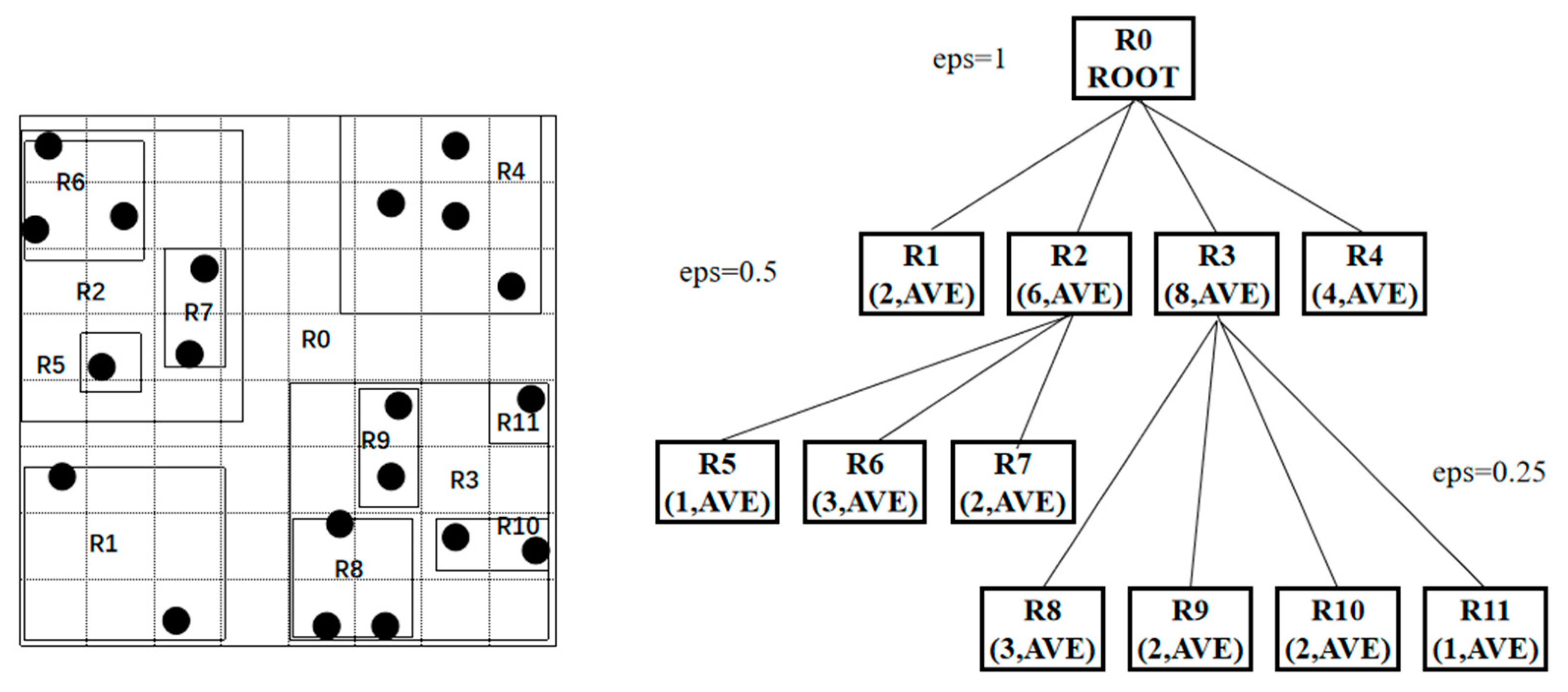
3.1. Structure of SbMBR Tree

To achieve lossy compression of spatial data according to a given maximum error, we use MBRs (minimum bounding rectangles) to partition the spatial data. An MBR contains data within a certain space range, as well as information about the average value of these data and the maximum error of these data [8]. In the process of compression, we select appropriate MBRs according to the given maximum acceptable error and use the average value contained in each selected MBR to replace the original data.

To realize the above-mentioned selection process quickly, we constructed an index tree for these MBRs. We call the index tree SbMBR tree. The structure of the SbMBR tree is similar to that of the R-tree. Each node in the SbMBR tree contains an MBR. The MBR in the child node is completely contained by the MBR of the parent node. The maximum error value contained in nodes at the same layer in the SbMBR tree is the same. The maximum error value contained in the node in the deeper position in the tree is smaller than that of the node in the shallow position. In particular, the root node contains the entire spatial data, and its maximum error value is the largest in the tree. An example of the structure of an SbMBR tree is shown in Figure 1.

The structure of the SbMBR tree will be described more formally below. Let $S=\left\{R_1,R_2,\dots ,R_n\right\}$ be a set of n MBRs in the plane. Each MBR contains six properties, namely, the x-coordinate of the bottom left corner $x_{\min }\left(R_i\right)$, the y-coordinate of the bottom left corner $y_{\min }\left(R_i\right)$, the x-coordinate of the top right corner $x_{\max }\left(R_i\right)$, the y-coordinate of the top right corner $y_{\max }\left(R_i\right)$, as well as the average value $\mu \left(R_i\right)$ and the maximum error $\epsilon \left(R_i\right)$ of the data in the area denoted by the bottom left and top right corners.

Definition 1. 

The union MBR P of two MBRs, $R_1,R_2$, is denoted by $P=R_1\cup R_2$; P satisfies:

$$x_{\min }\left(P\right)=\min \left(x_{\min }\left(R_1\right),x_{\min }\left(R_2\right)\right)$$

(1)

$$y_{\min }\left(P\right)=\min \left(y_{\min }\left(R_1\right),y_{\min }\left(R_2\right)\right)$$

(2)

$$x_{\max }\left(P\right)=\max \left(x_{\max }\left(R_1\right),x_{\max }\left(R_2\right)\right)$$

(3)

$$y_{\max }\left(P\right)=\max \left(y_{\max }\left(R_1\right),y_{\max }\left(R_2\right)\right)$$

(4)

where $\mu \left(P\right)$ is the average value of the data in the area denoted by the bottom left corner $\left(x_{\min }\left(P\right),y_{\min }\left(P\right)\right)$ and the top right corner $\left(x_{\max }\left(P\right),y_{\max }\left(P\right)\right)$, and $\epsilon \left(P\right)$ is the maximum error of the data in the area denoted by the bottom left corner $\left(x_{\min }\left(P\right),y_{\min }\left(P\right)\right)$ and the top right corner $\left(x_{\max }\left(P\right),y_{\max }\left(P\right)\right)$.

The SbMBR tree $T_S$ on S is defined as follows: Each node of the SbMBR tree contains only one MBR. All the elements of S are leaf nodes in the SbMBR tree $T_S$. If S contains only one MBR, $T_S$ contains only one single leaf node; otherwise, we use some packing algorithm mentioned below to partition set S into some disjointed subsets. Without loss of generality, we assume that set S is partitioned into $S_1,S_2,\dots ,S_k$, where ${\displaystyle \underset{i=1}{\overset{k}{\cup }}{S}_i}=S$,$S_i\cap S_j=\varnothing ,i\ne j,i,j=1,2,\dots ,k$. Let $P_i={\displaystyle \underset{R\in S_i}{\cup }R}$, which means that $P_i$ is the union MBR of all elements in $S_i$. Let $P=\left\{P_1,P_2,\dots ,P_k\right\}$. $T_S$ is derived from the recursive SbMBR tree $T_P$. For each leaf node $P_i$ of the tree $T_P$, let all the elements in $S_i$ be the child nodes of $P_i$, so that $T_S$ is constructed, whose leaf nodes are all in the set $S$.

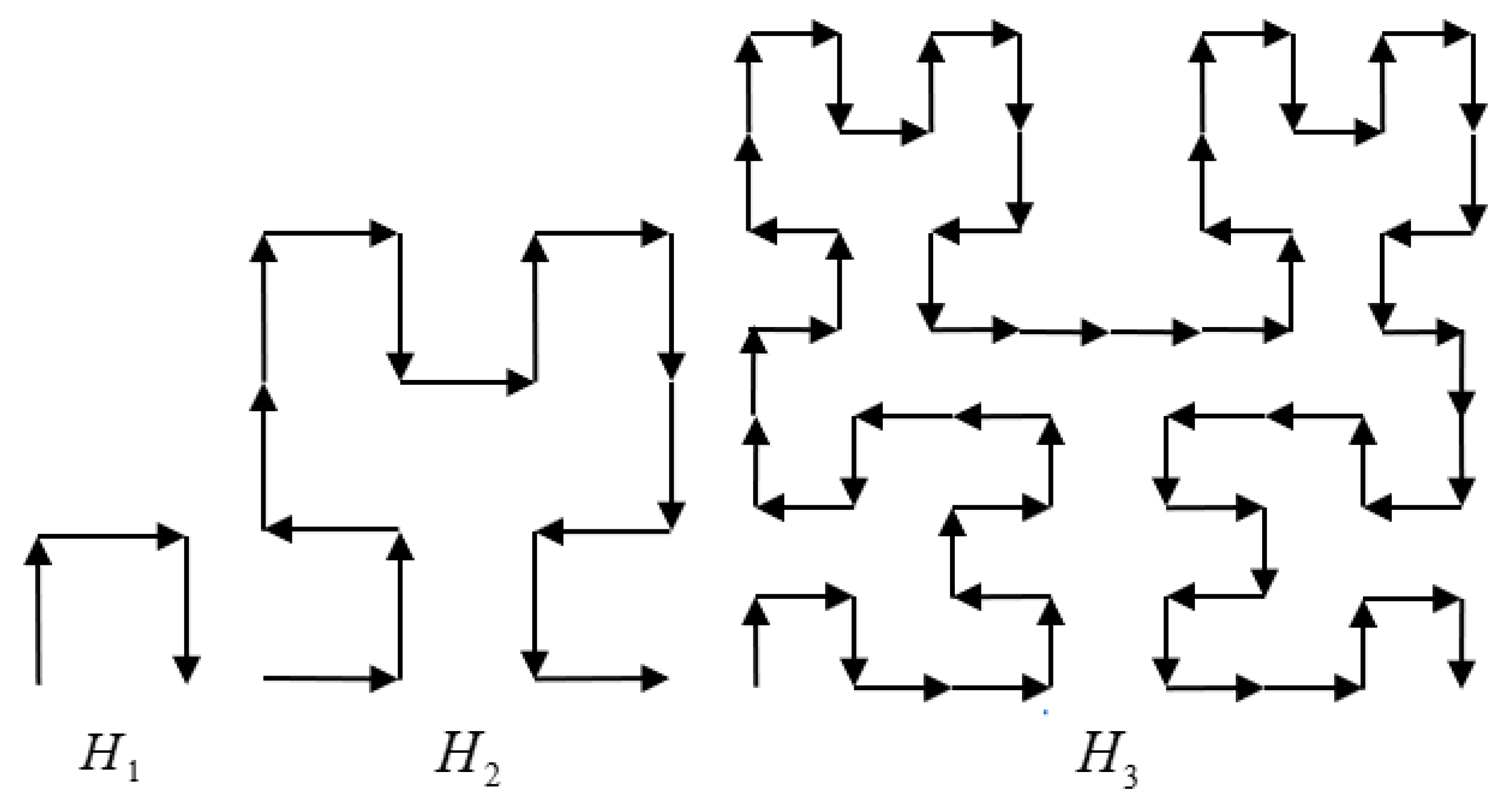
3.2. Construct MBRs with Hilbert Curve

In order to construct the SbMBR tree mentioned above, the key is to construct MBRs with larger maximum error values according to existing MBRs with smaller maximum error values. In this paper, we propose a heuristic method similar to the method used in Hilbert R-tree to realize it [31].

A Hilbert curve is a kind of space-filling curve which can visit all the points in a k-dimensional grid exactly once and never crosses. As shown in Figure 2, the basic Hilbert curve, also called the curve of order 1, is on a 2 × 2 grid, denoted by H₁. The curve of order i is derived from four curves of order i − 1 with different orientations. The second-order and third-order Hilbert curve are also shown in Figure 2. When the order of a Hilbert curve gradually increases until it reaches infinity, the curve becomes fractal [26].

The path of a Hilbert space-filling curve gives the multi-dimensional grid points a one-dimensional linear order, which makes it as easy to process the data in multi-dimensional space as in one-dimension space.

Next, we propose a method to construct MBRs with the Hilbert curve. It is assumed that the maximum error value of the MBRs to be constructed has been given. First, we sort the existing MBRs according to their centers in the order of the Hilbert curve. Second, we scan backward from the first MBR until the n-th MBR is scanned and the maximum error value of the first n MBRs is just greater than the given maximum error value. Therefore, the first n − 1 MBRs can be merged into a larger MBR whose error value is not larger than the given maximum error value. Then, we repeat the above operation with the n-th MBR as the first MBR until all the existing MBRs are processed. The specific algorithm pseudocode is shown in Algorithm 1.

Algorithm 1: Merge MBRs with the Hilbert curve

Input: A set of MBRs with the same maximum error value p, the maximum error of new MBRs to be obtained x Output: A set of new MBRs with given maximum error value; inclusion relationship between new MBRs to be obtained and existing MBRs

S←$\varnothing$ R←$\varnothing$ sort p according to their centers with the Hilbert curve i←0 j←0 while i < p.size do   while j < p.size do     y←calculate the maximum error of the MBR of pi, pi+1, …, pj     if y > x then       break     end if     j←j + 1   end while   m←calculate the MBR of pi, pi+1, …, pj−1   S.insert(m)   for k = i, i + 1, …, j − 1 do     R.insert(pk)$\subseteq m$   end for   i←j end while return (S, R)

Hilbert curves have good clustering properties, that is, they maintain locality between objects in a multidimensional space in a linear one-dimensional space [32]. Such good properties are very consistent with the requirements under the spatial data scenario. Similarly, the z-order curve is an alternative that possesses similar properties to the Hilbert curve. However, experiments show that the z-order curve underperforms the Hilbert curve in queries for a certain number of points with triangular regions [27].

The above is mainly about the two-dimensional Hilbert curve. A Hilbert curve can be conveniently extended to three dimensions or higher dimensions. A three-dimensional Hilbert curve is shown in Figure 3. The extension method is described in detail in [32].

3.3. Indexing Algorithm

Algorithm 2 presents the tree-building algorithm for an SbMBR tree. To implement it, we use the bottom-up tree construction method. First, we regard spatiotemporal data as several 1 × 1 MBRs. Then, Algorithm 1 is continuously used to merge MBR to the upper layer, where the maximum error of each layer increases in the form of multiplication. At the same time, the relationship between the upper and lower layers is established. Until all MBRs are merged into one MBR, the MBR is the root node of the SbMBR tree.

Algorithm 2: Build SbMBR tree

Input: spatial data D, the maximum error of leaf nodes x Output: the SbMBR tree

T←$\varnothing$ p←transform D into MBRs whose size is 1 × 1 and the maximum error is x T.addNode(p) while p.size > 1 do   x←2x   (q, R)←merge_MBR(p, x)    //Algorithm 1   T.addNode(q)   T.addEdge(R)   p←q end while return T

A range query receives a query rectangle range and maximum acceptable maximum error and returns a set of MBRs who can fill the space of the rectangle range and meet the requirement of maximum error.

Algorithm 3 describes the range query algorithm. We mainly use recursive methods to realize error-controllable range queries. I is the intersection of the MBR of the current node and the query range. When I is empty, no MBRs are meeting the query requirement, so an empty set is returned. When I is not empty and eps of the MBR of the current node is less than or equal to the given eps, I has satisfied the requirement, so I is returned. Notably, when the root node has no child, even if the error does not meet the condition, only I can be returned. After the above conditions are eliminated, recursion calling is required.

Algorithm 3: Range query

Input: the root node of a subtree root, rectangle range R, maximum error eps Output: A set of MBRs contained in range R

S←$\varnothing$ I←$R\cap root.MBR$ if $I=\varnothing$ then   return $\varnothing$ end if if $root.MBR.eps\le eps$ or the root node has no child then   return I end if for ch in all the children of root do   S←$S\cup$range_query(ch, R, eps)    //recursive function call end for return S

3.4. Error Estimation Method for Data Analysis

In order to better apply the methods mentioned above to data analysis, it is necessary to establish error estimation methods to estimate the errors after data analysis or prediction [33].

Assume that in a data analysis model, the input is X and the output is Y. This model essentially maps X to Y, and if this mapping is f, the model can be expressed as follows:

$$Y=f\left(X\right)$$

(5)

where X is the input and Y is the output.

When compressing the input X, the accuracy of the output Y will decrease. This section proposes a method for error estimation based on normalized mutual information.

3.4.1. Mutual Information

Mutual information is a measure of the mutual dependence between two random variables. The mutual information of two discrete random variables X and Y, namely,$I\left(X;Y\right)$, can be calculated as follows:

$$I\left(X;Y\right)={\displaystyle \sum _{y\in Y}{\displaystyle \sum _{x\in X}{P}_{\left(X,Y\right)}\left(x,y\right)}\log \left(\frac{P_{\left(X,Y\right)}\left(x,y\right)}{P_X\left(x\right)P_Y\left(y\right)}\right)}$$

(6)

where $P_{\left(X,Y\right)}$ is the joint probability mass function of X and Y, and $P_X$ and $P_Y$ are the marginal probability mass function of X and Y, respectively.

In this section, X is the result of compressing the input and Y is the original output.

3.4.2. Normalization

In order to make the metric for error estimation comparable to different data, it should be normalized.

The mutual information can be expressed in the form of entropy, as follows:

$$I\left(X;Y\right)=H\left(X\right)+H\left(Y\right)-H\left(X,Y\right)$$

(7)

where $H$ is the entropy function.

Therefore, the normalized mutual information of random variables X and Y can be defined as below:

$$U\left(X;Y\right)=\frac{2I\left(X;Y\right)}{H\left(X\right)+H\left(Y\right)}$$

(8)

where X and Y are both random variables.

In summary, the metric for error estimation can be calculated as follows:

$$U\left(X;Y\right)=\frac{2{\displaystyle \sum _{y\in Y}{\displaystyle \sum _{x\in X}{P}_{\left(X,Y\right)}\left(x,y\right)\log \left(\frac{P_{\left(X,Y\right)}\left(x,y\right)}{P_X\left(x\right)P_Y\left(y\right)}\right)}}}{{\displaystyle \sum _{x\in X}{P}_X\left(x\right)\log \left(P_X\left(x\right)\right)}+{\displaystyle \sum _{y\in Y}{P}_Y\left(y\right)\log \left(P_Y\left(y\right)\right)}}$$

(9)

where X is the input data, Y is the output data, $P_{\left(X,Y\right)}$ is the joint probability mass function of X and Y, and $P_X$ and $P_Y$ are the marginal probability mass function of X and Y, respectively.

The range of the normalized mutual information is from 0 to 1. The closer the normalized mutual information value is to 1, the higher the correlation is and vice versa.

Therefore, we will use U(X;Y), namely, normalized mutual information, as the indicator of error estimation.

3.5. Complexity Analysis

Lemma 1. 

The time complexity of merging n MBRs with the Hilbert curve is $O\left(n\right)$.

Proof. 

We assume that the cost of merging two MBRs is constant time. Because variables i and j in Algorithm 1 only increase in the loop, the maximum number of loops is $2n$, and the time complexity of Algorithm 1 is $O\left(n\right)$. □

Lemma 2. 

In the case where $k\left(k>1\right)$ MBRs can be merged into 1 MBR on average, the time complexity of building the SbMBR tree of data of scale n is $O\left(\frac{kn}{k-1}\right)$.

Proof. 

According to Lemma 1, all the operations in the loop of Algorithm 2 are linear in time. Therefore, the time cost can be denoted as the size of the SbMBR tree. The size of the SbMBR tree S can be estimated as below:

$$S={\displaystyle \sum _{i=0}^{⌈{\log }_{k}n⌉}\frac{n}{k^i}}\le n{\displaystyle \sum _{i=0}^{\infty }\frac{1}{k^i}=\frac{kn}{k-1}}$$

(10)

Therefore, the time complexity of building the SbMBR tree of data of scale n is $O\left(\frac{kn}{k-1}\right)$. □

Lemma 3. 

Under the circumstance that the compression ratio with an error of $\epsilon$ is denoted as $r\left(\epsilon \right)$, and $k\left(k>1\right)$ MBRs can be merged into 1 MBR on average, the time complexity of range query of size n is $O\left(r\left(\epsilon \right)n{\log }_{k}n\right)$.

Proof. 

The answer of Algorithm 3 can be considered to be a subset of MBRs in a certain layer. When the compression ratio is $r\left(\epsilon \right)$, the size of the result MBRs is $nr\left(\epsilon \right)$. According to the feature of the tree structure, the depth of the certain layer is ${\log }_{k}n$. In addition, the complexity of the recursive algorithm merging process is linear complexity. According to the master theorem, the time complexity is $O\left(r\left(\epsilon \right)n{\log }_{k}n\right)$. □

4. Experimentation and Results

4.1. Experimental Setup

To assess the merit of our proposed SbMBR tree with the Hilbert curve, we implemented and ran experiments on a two-dimensional space. The method was implemented in C++, under Linux. We compared our method against the quadtree [8] and brute R-tree. The brute R-tree method is a method that uses an index structure similar to the SbMBR tree but uses the $O\left(n^2\right)$ brute method instead of the Hilbert curve in the process of MBR merging. In addition, we also compared our method with the JPEG compression algorithm in machine learning scenarios.

The hardware specification is listed below:

• Processor: Intel© Core© i7-10875H CPU @ 2.30 GHz
• RAM: 16 GB
• OS: Ubuntu 22.04

The test data set used in the experiment is WorldClim version 2.1 climate data for 1970–2000 [34]. We mainly chose the data of the average temperature in July and solar radiation in April. Total

Table 1. Details of data for the experiment.

Name of the Data	Types of the Data	Location of the Data	Density of the Data	Scale of the Data
Test 1	Average temperature in July	31°40′ N–48°20′ N, 96°40′ W–80°00′ W	Dense	400 × 400
Test 2	Average temperature in July	30°00′ S–6°40′ N, 180°00′–138°20′ W	Sparse	880 × 1000
Test 3	Solar radiation in April	33°45′ N–50°25′ N, 100°50′ W–75°50′ W	Dense	600 × 400
Test 4	Solar radiation in April	30°00′ S–6°40′ N, 180°00′–138°20′ W	Sparse	880 × 1000

shows the details of the data for the experiment.

Table 2. Params used in all the methods.

Method	Param Name	Explanation	Value Range or Requirement
SbMBR tree	eps array	eps of different layers when building the SbMBR tree	$\left[0,+\infty \right)$, incremental
	query eps	eps of query area	$\left[0,+\infty \right)$
	query area	a rectangle area needed to query, containing the coordinate of the bottom left corner and top right corner	Coordinates of two real number points
brute R-tree	eps array	eps of different layers when building the tree	$\left[0,+\infty \right)$, incremental
	query eps	eps of query area	$\left[0,+\infty \right)$
	query area	a rectangle area needed to query, containing the coordinate of the bottom left corner and top right corner	Coordinates of two real number points
quadtree	query eps	eps of query area	$\left[0,+\infty \right)$
	query area	a rectangle area needed to query, containing the coordinate of the bottom left corner and top right corner	Coordinates of two real number points
JPEG	ratio	compression ratio	$\left[0,1\right]$

explains the details of the params used in all the methods when we experimented.

In our implementation, we used the coefficient of variation as eps in our algorithm. The specific definition is as follows:

$$eps=\frac{\sigma }{\mu }$$

(11)

where $\sigma$ is the standard deviation and $\mu$ is the average value. Different eps can also show the advantages and limitations of the methods.

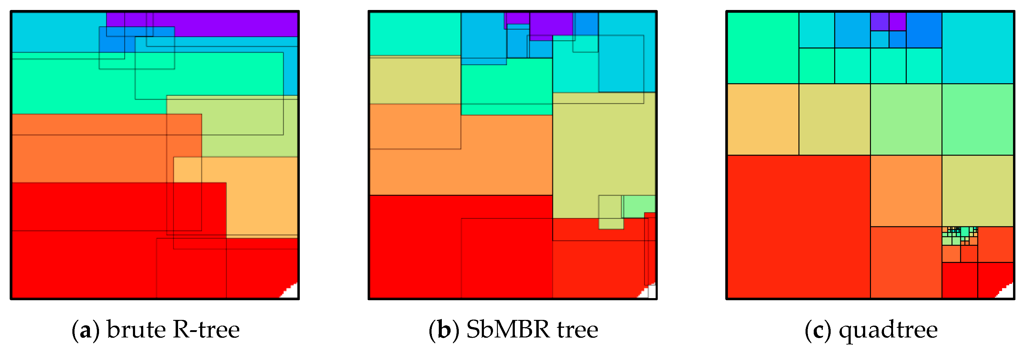
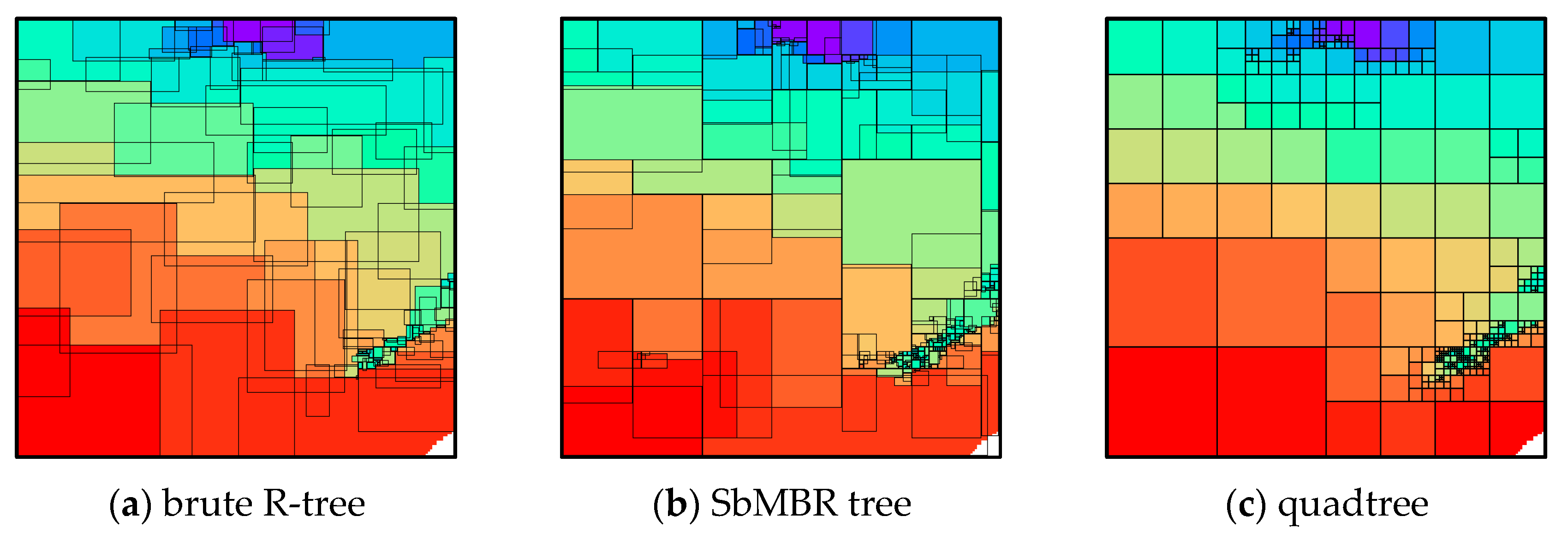
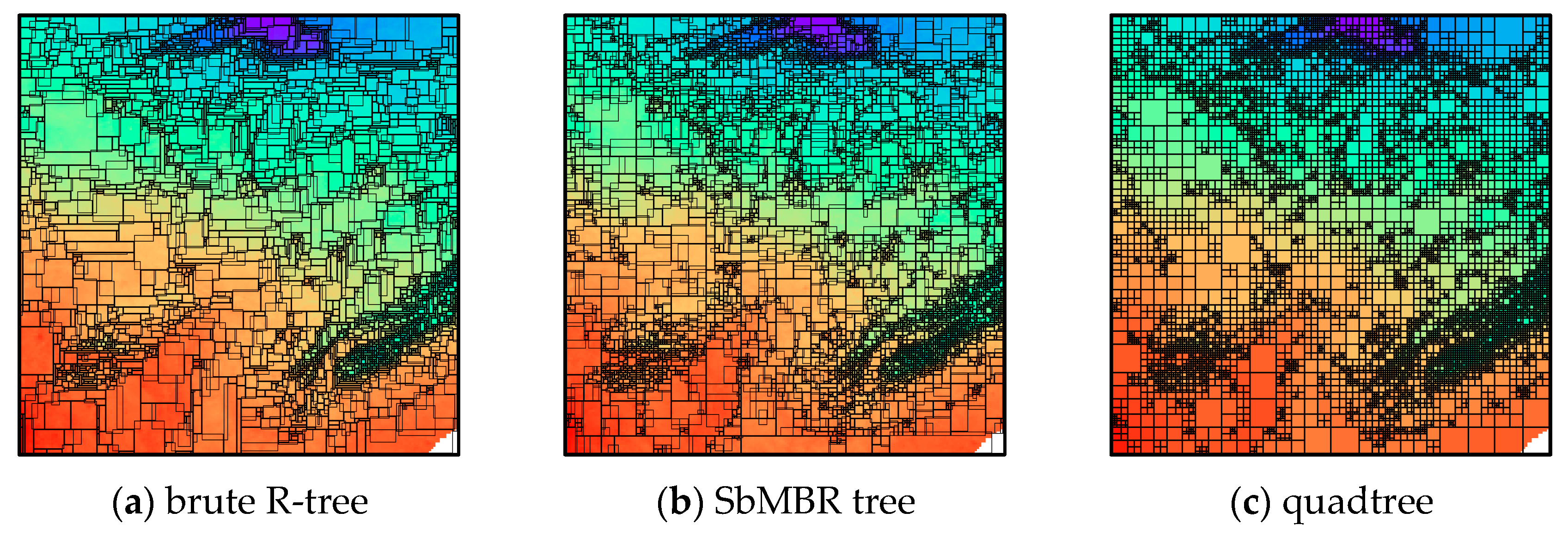
4.2. Visualization of Compression Results

Figure 4, Figure 5 and Figure 6 show the effect of drawing the compressed data back to the metadata. Each boxed area in the figure represents that all data in that area can be replaced by one data point, thus achieving the compression effect. The rectangular boxed-out intersection section then represents the location with a variety of different choices that are feasible for a given error range.

From Figure 4, Figure 5 and Figure 6, we can see that the major drawback of the quadtree is that all regions of its partition are square, which seriously affects the flexibility of compression and results in too many points in regions with more complex data, while the SbMBR tree and brute R-tree solve such a problem by rectangular partitioning. In addition, the SbMBR tree circumvents the overlapping of too many matrices, which increases the compression ratio and query speed.

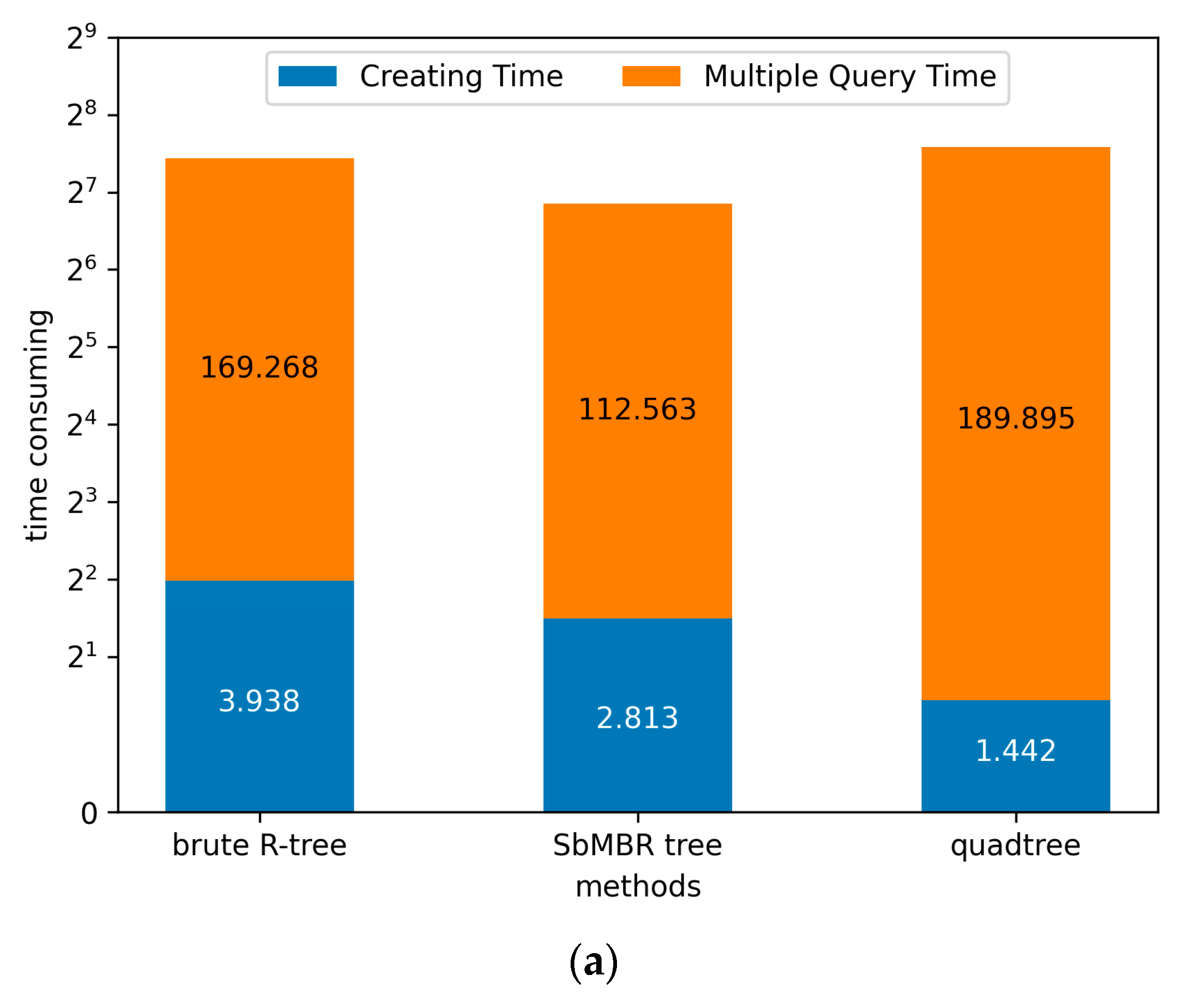
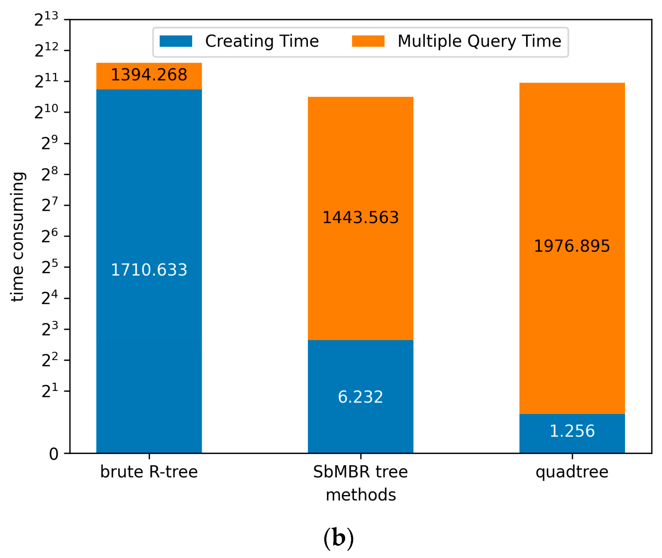
4.3. Comparison of Index Construction and Data Query Efficiency

To compare our proposed SbMBR tree with quadtree and brute R-tree, we performed about 150,000 random queries with an allowable error of 0.1% to 0.5% on data of different densities and recorded the creating time and query time for different methods. The temporal information is analyzed in Figure 7, where Figure 7a represents the performance of each method in sparse data and Figure 7b represents the performance of each method in dense data.

In the

Table 3. Relative time of different methods under the same sparse data.

Method	Relative Time of Creating Tree	Relative Time of Multiple Querying	Relative Total Time
quadtree	100.0%	100.0%	100.0%
SbMBR tree	195.1%	59.2%	60.2%
brute R-tree	273.1%	89.1%	90.5%

and

Table 4. Relative time of different methods under the same dense data.

Method	Relative Time of Creating Tree	Relative Time of Multiple Querying	Relative Total Time
quadtree	100.0%	100.0%	100.0%
SbMBR tree	496.1%	73.0%	73.2%
brute R-tree	136,196.9%	70.5%	156.9%

, relative time can be defined as follows:

$$RelativeTime=\frac{t}{t_0}$$

(12)

where t means the absolute time of different methods and t₀ means the fiducial time; in this case, the time scale of the quadtree is the fiducial time.

A comprehensive analysis of Figure 7 and Table 3 and Table 4 show that the brute R-tree always leads to more time spent than the SbMBR tree and quadtree in construction, and even more so in the case of dense data. In addition, although the quadtree shows a better construction speed, its query speed is slow and will be a serious shortcoming in large-scale queries, and the SbMBR tree seems to outperform the other methods in general.

From analyzing the reason, we can see that the bottleneck of the brute R-tree is that it needs to traverse all the neighboring information to calculate and update the MBR, which will lead to an order of magnitude increase in time complexity compared with other methods. Each internal node has exactly four children in a quadtree, so a quadtree should not spend time considering the surrounding data, but rather should keep recursion down. So, quadtree has the best construction consumption. However, although brute R-tree spends so much time in construction, the detailed nodes’ information makes it query recursive depth lower and more efficient to query. On the contrary, the simple splitting of the quadtree makes the overall depth higher, and the query must recurse more layers.

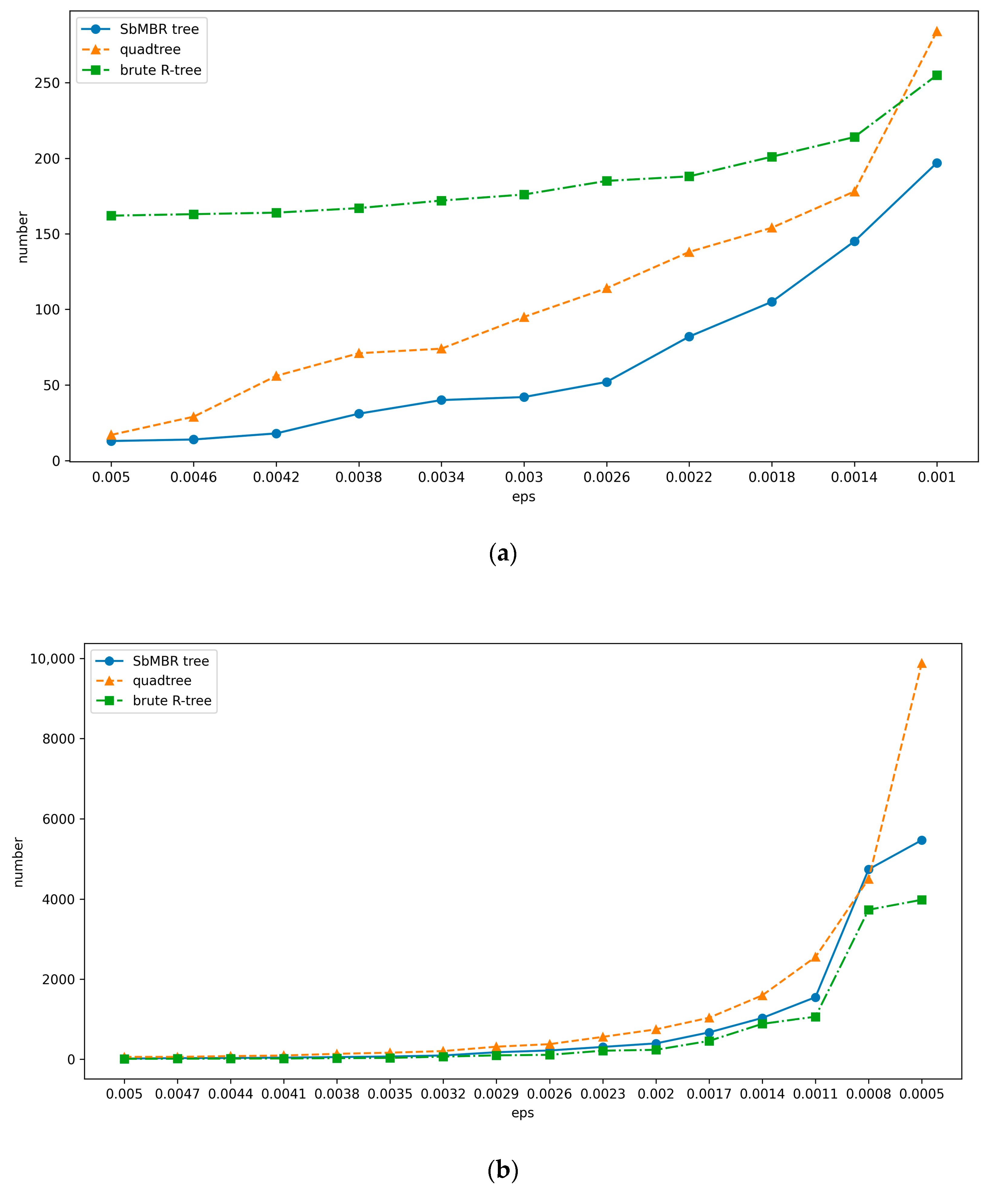
4.4. Comparison of Compression Ratio and Nodes Number

To further identify the advantages and disadvantages of different methods, we counted the number of nodes compressed with different data and different error ranges. The number of nodes will visually show the compression efficiency.

In

Table 5. Volume reduction ratio of different methods under the same sparse data.

eps	Method	Volume Reduction Ratio
0.005	SbMBR tree	0.000236
	brute R-tree	0.002945
	quadtree	0.000309
0.0046	SbMBR tree	0.000254
	brute R-tree	0.002963
	quadtree	0.000527
0.0042	SbMBR tree	0.000327
	brute R-tree	0.002981
	quadtree	0.001018
0.0038	SbMBR tree	0.000563
	brute R-tree	0.003036
	quadtree	0.001290
0.0034	SbMBR tree	0.000727
	brute R-tree	0.003127
	quadtree	0.001345
0.003	SbMBR tree	0.000763
	brute R-tree	0.003200
	quadtree	0.001727
0.0026	SbMBR tree	0.000945
	brute R-tree	0.003363
	quadtree	0.002072
0.0022	SbMBR tree	0.001490
	brute R-tree	0.003418
	quadtree	0.002509
0.0018	SbMBR tree	0.001909
	brute R-tree	0.003654
	quadtree	0.002800
0.0014	SbMBR tree	0.002636
	brute R-tree	0.003890
	quadtree	0.003236
0.001	SbMBR tree	0.003581
	brute R-tree	0.004636
	quadtree	0.005163

and

Table 6. Volume reduction ratio of different methods under the same dense data.

eps	Method	Volume Reduction Ratio
0.005	SbMBR tree	0.0018
	brute R-tree	0.0011
	quadtree	0.0060
0.0047	SbMBR tree	0.0030
	brute R-tree	0.0015
	quadtree	0.0060
0.0044	SbMBR tree	0.0032
	brute R-tree	0.0017
	quadtree	0.0080
0.0041	SbMBR tree	0.0042
	brute R-tree	0.0021
	quadtree	0.0100
0.0038	SbMBR tree	0.0056
	brute R-tree	0.0028
	quadtree	0.0140
0.0035	SbMBR tree	0.0071
	brute R-tree	0.0035
	quadtree	0.0170
0.0032	SbMBR tree	0.0096
	brute R-tree	0.0067
	quadtree	0.0210
0.0029	SbMBR tree	0.0176
	brute R-tree	0.0099
	quadtree	0.0320
0.0026	SbMBR tree	0.0221
	brute R-tree	0.0112
	quadtree	0.0380
0.0023	SbMBR tree	0.0309
	brute R-tree	0.0215
	quadtree	0.0560
0.002	SbMBR tree	0.0397
	brute R-tree	0.0237
	quadtree	0.0750
0.0017	SbMBR tree	0.0672
	brute R-tree	0.0459
	quadtree	0.1040
0.0014	SbMBR tree	0.1032
	brute R-tree	0.0885
	quadtree	0.1600
0.0011	SbMBR tree	0.1550
	brute R-tree	0.1064
	quadtree	0.2550
0.0008	SbMBR tree	0.4742
	brute R-tree	0.3733
	quadtree	0.4500
0.0005	SbMBR tree	0.5471
	brute R-tree	0.3982
	quadtree	0.9880

, volume reduction ratio can be defined as follows:

$$VolumeReductionRatio=\frac{sum}{su{m}_0}$$

(13)

where sum means the size of data after being compressed and sum₀ means the initial data size.

The results of our test are shown in Figure 8 and Table 5 and Table 6. The experimental comparison results for sparse data are in Figure 8a and for dense data are in Figure 8b. For the brute R-tree, it can be seen via the sparse and dense data that the number of nodes of the brute R-tree generally remains stable for different error ranges, with more nodes in the sparse data and fewer nodes in the dense data. The quadtree has a better compression ratio at a larger error tolerance. However, when the error tolerance becomes smaller, the number of nodes of the quadtree immediately grows massively, far exceeding the brute R-tree and SbMBR tree. The SbMBR tree has the best performance in sparse data, while guaranteeing the construction speed and compression ratio in dense data. Overall, it is the most stable and efficient.

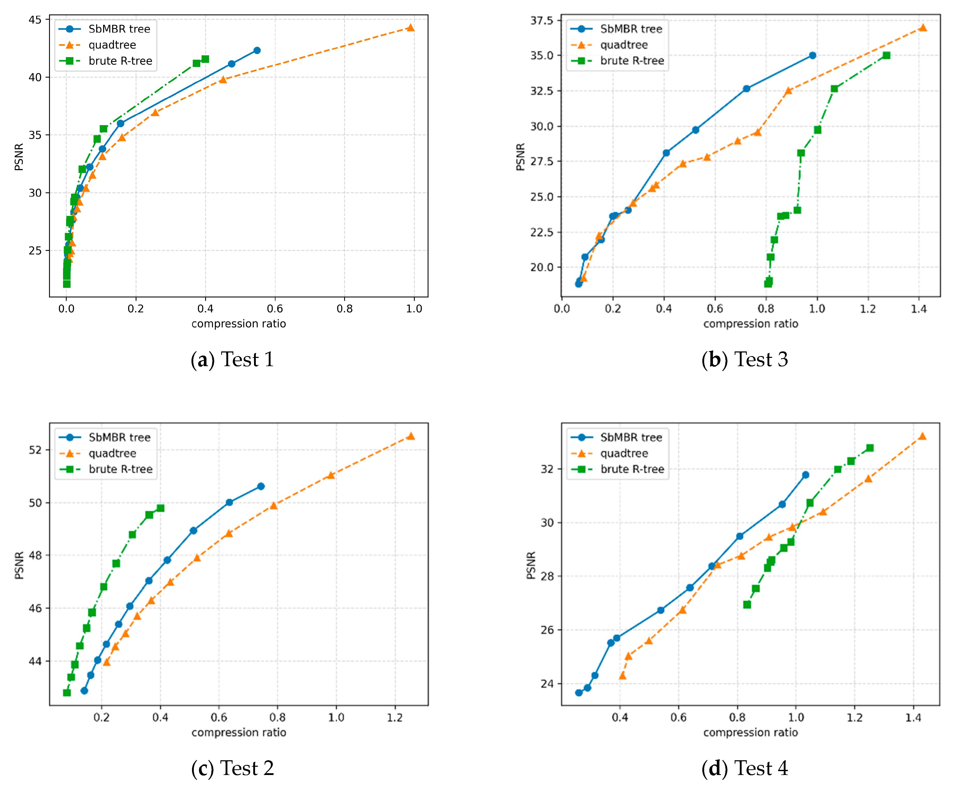
4.5. Comparison of Peak Signal-to-Noise Ratio (PSNR) under the Same Compression Ratio

The peak signal-to-noise ratio (PSNR) measures the difference between the original and compressed versions of an image or video in terms of the peak signal power and the amount of noise introduced during the compression process. The PSNR–compression ratio curve serves as a visual tool to understand the trade-offs between compression and quality in a compression algorithm and to evaluate its performance compared to other algorithms.

PSNR can be defined as follows:

$$PSNR=10\cdot {\log }_{10}\left(\frac{{\left(m-n\right)}^2}{e}\right)$$

(14)

where m means the max value in the data set, n means the min value in the dataset, and e means the mean-square error between the compressed data and the origin data.

Figure 9 shows the comparison results between methods based on the SbMBR tree, quadtree, and brute R-tree. The meanings of Test 1, Test 2, Test 3, and Test 4 are described in detail in Section 4.1.

The data used in Test 1 and Test 3 are dense, while the data used in Test 2 and Test 4 are sparse. In sparse data, the method based on the SbMBR tree is generally superior to the method based on quadtree and brute R-tree. And in dense data, the method based on the SbMBR tree is generally superior to the method based on quadtree, but inferior to the method based on brute R-tree.

4.6. Case Study of Using SbMBR Tree in Data Analysis

To demonstrate the effectiveness of the error control method, we provided a case study where the SbMBR tree is applied in a typical data analysis scenario. The typical data we used is the precipitation in January, February, March, and April from 2017 to 2019 in WorldClim version 2.1 climate data for 1970–2000 [34]. In this section, we always regard the compressed data of the precipitation in January, February, and March as the model input, and the precipitation in April as the model output.

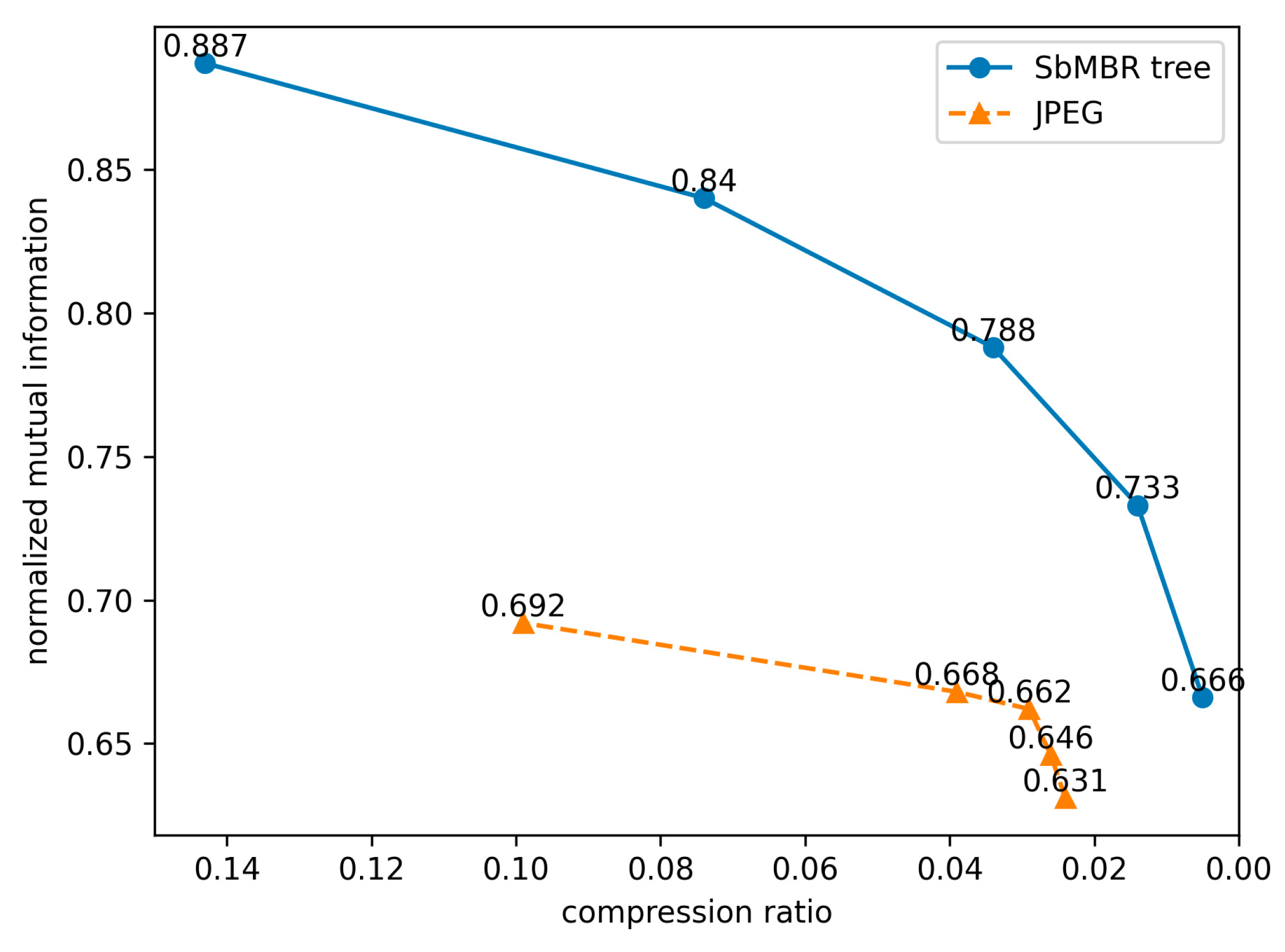
4.6.1. Results of Error Estimations

We used the SbMBR tree algorithm and JPEG algorithm with different parameters to compress the precipitation in January, February, and March. Then, we used the error estimation method mentioned in Section 3.3 to calculate the normalized mutual information. The result is shown in Figure 10 in the form of the normalized mutual information–compression ratio curve.

From Figure 10, it can be concluded that with the compression ratio decreasing, the mutual dependence between compressed data and real data decreases, which means a low compression ratio leads to high error. In addition, using the SbMBR tree will result in higher similarity than using the JPEG algorithm at the same compression ratio.

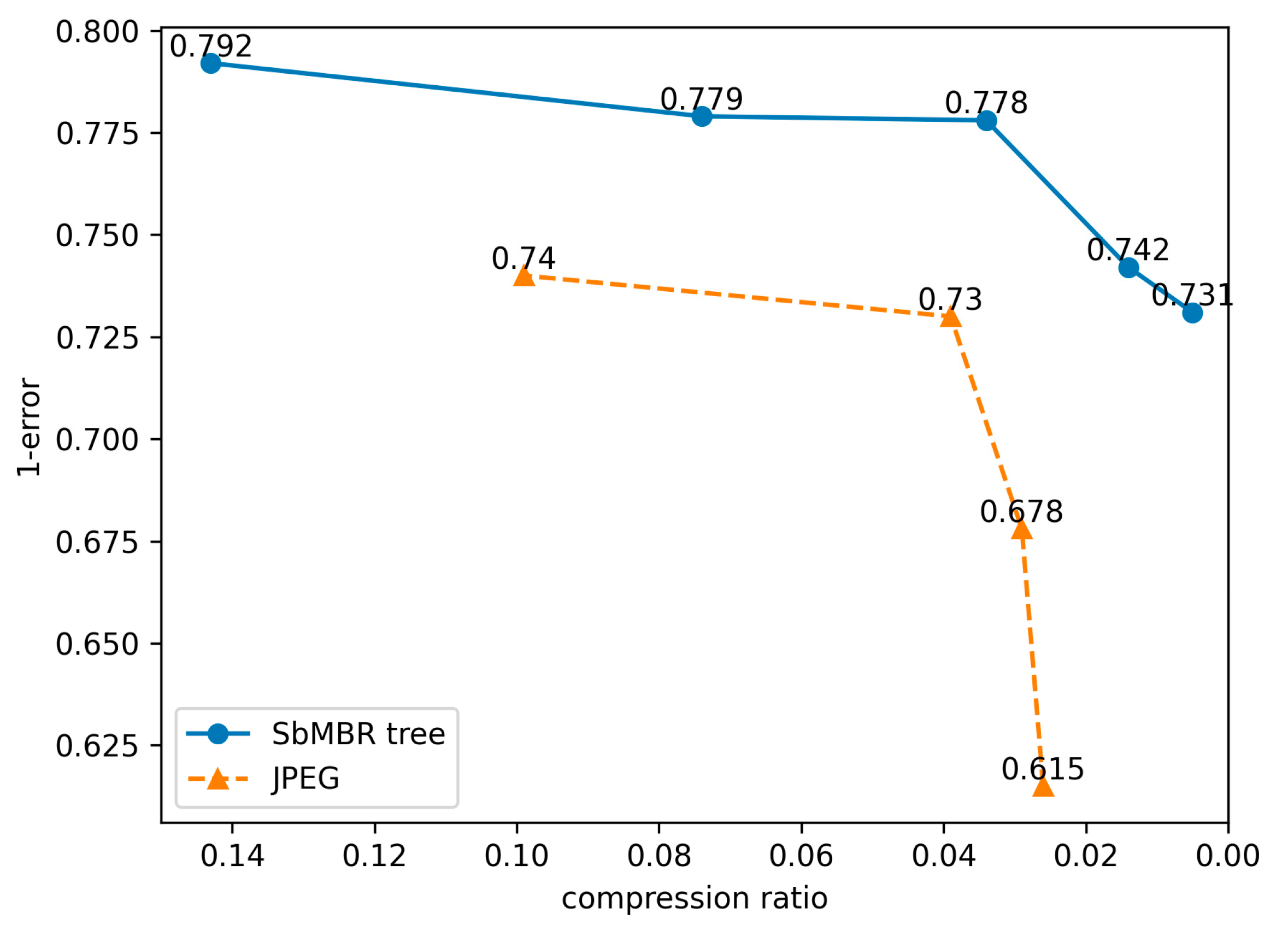
4.6.2. Validation of Error Estimation Method

To further validate our error estimation method, we used the ConvLSTM [35] model to predict the precipitation in April by the precipitation after compression in January, February, and March. The parameters of the ConvLSTM model are shown in

Table 7. Params used in ConvLSTM.

Param Name	Value
Convolution kernel	3 × 3
Number of Convolutional layers	4
Number of nodes per layer	{1,16,32,64}
Optimizer	AdamW
Loss Function	L1Loss

.

Firstly, we used the SbMBR tree algorithm and JPEG algorithm, respectively, to compress the data of the precipitation in January, February, March, and April in 2017, 2018, and 2019.

Secondly, we spitted the rasterized data into many 216 × 216 submatrices. Then, we used the precipitation in January, February, and March as the input and used the compressed precipitation in April as the output to train with the ConvLSTM model.

We simply defined $1-error$ as follows:

$$1-error=avg\left(\frac{\left|x-x_{org}\right|}{x_{org}+p}\right)$$

(15)

where $x_{org}$ is the original data, $x$ is the compressed data, $p$ is a small constant number used to avoid $x_{org}+p=0$, and $avg$ is the average value function.

After training, we obtained the predicted data from the compressed input. Then, we calculated the $1-error$ mentioned above for all the inputs. The result is shown in Figure 11 in the form of the $1-error$–compression ratio curve.

From Figure 11, it can be concluded that with the compression ratio growing, the 1–error between compressed data and real data increases, which is consistent with the result in Section 4.6.1. In addition, the curve of the SbMBR tree is overall above the curve of JPEG, which is also consistent with the result in Section 4.6.1.

To sum up, our error estimation method is effective on these meteorological data, and our compression method performs better than the JPEG algorithm on these meteorological data.

5. Conclusions

In this paper, we propose the SbMBR tree, a novel indexing and error-bounded lossy compression method for spatiotemporal data. The proposed method hierarchically divides the data space into several MBRs through Hilbert curves and builds an indexing structure on this basis. The range query algorithm in the SbMBR tree is also presented. For cross-domain data mining and analysis scenarios, mutual information is used to estimate information loss. We evaluate the performance of our proposed methods on three of the most important aspects, including computational efficiency, compression ratio, and data utility. The results are compared with some of the typical indexing and compression algorithms, and the summaries are: (1) the loss control mechanism is unique among existing tree-indexed lossy compression algorithms; (2) the compression algorithm based on the SbMBR tree has slightly better compression performance compared to the quadtree and JPEG algorithms; (3) the overall efficiency of the building and querying SbMBR trees is slightly better than that of quadtree and brute R-tree; (4) the error estimation method based on mutual information proposed in this paper is consistent with the real error. Overall, our results are promising in that the SbMBR tree might be more efficient if it is applied to data sets that contain larger spatiotemporal regions with high local similarities.

References

1. Foster, I.; Ainsworth, M.; Allen, B.; Bessac, J.; Cappello, F.; Choi, J.Y.; Constantinescu, E.; Davis, P.E.; Di, S.; Di, W.; et al. Computing Just What You Need: Online Data Analysis and Reduction at Extreme Scales. In Proceedings of the European Conference on Parallel Processing (Euro-Par 2017), Jaipur, India, 23 June 2017; pp. 3–19. [Google Scholar]
2. Lee, J.-G.; Kang, M. Geospatial big data: Challenges and opportunities. Big Data Res. 2015, 2, 74–81. [Google Scholar] [CrossRef]
3. Huo, H.; Long, P.; Vitter, J.S. Practical High-Order Entropy-Compressed Text Self-Indexing. IEEE Trans. Knowl. Data Eng. 2023, 35, 2943–2960. [Google Scholar] [CrossRef]
4. Ghosh, S.; Eldawy, A. AID*: A Spatial Index for Visual Exploration of Geo-Spatial Data. IEEE Trans. Knowl. Data Eng. 2022, 34, 3569–3582. [Google Scholar] [CrossRef]
5. Kim, M.; Liu, L.; Choi, W. Multi-GPU Efficient Indexing for Maximizing Parallelism of High Dimensional Range Query Services. IEEE Trans. Serv. Comput. 2022, 15, 2910–2924. [Google Scholar] [CrossRef]
6. Andrés, F.-R.; Eduardo, R.-M.; Carlos, A.-C.; Fidel, L.-S. Image Retrieval System based on a Binary Auto-Encoder and a Convolutional Neural Network. IEEE Lat. Am. Trans. 2020, 18, 1925–1932. [Google Scholar] [CrossRef]
7. Moon, A.; Kim, J.; Zhang, J.; Son, S.W. Lossy compression on IoT big data by exploiting spatiotemporal correlation. In Proceedings of the 2017 IEEE High Performance Extreme Computing Conference (HPEC), Waltham, MA USA, 12–14 September 2017; IEEE: Piscataway, NJ, USA, 2017. [Google Scholar]
8. Jo, B.; Jung, S. Quadrant-based minimum bounding rectangle-tree indexing method for similarity queries over big spatial data in HBase. Sensors 2018, 18, 3032. [Google Scholar] [CrossRef] [PubMed]
9. Error-controlled lossy compression optimized for high compression ratios of scientific datasets. In Proceedings of the 2018 IEEE International Conference on Big Data (Big Data), Seattle, WA, USA, 10–13 December 2018; IEEE: Piscataway, NJ, USA, 2018.
10. Wang, Z.; Guan, R.; Pan, X.; Song, B.; Zhang, X.; Tian, Y. Efficient Spatiotemporal Big Data Indexing Algorithm with Loss Control. In Proceedings of the International Conference on Big Data and Security, Osaka, Japan, 17–20 December 2022; Springer Nature: Singapore, 2022; pp. 524–533. [Google Scholar]
11. Ainsworth, M.; Tugluk, O.; Whitney, B.; Klasky, S. Multilevel techniques for compression and reduction of scientific data—The univariate case. Comput. Vis. Sci. 2018, 19, 65–76. [Google Scholar] [CrossRef]
12. Lindstrom, P. Fixed-Rate Compressed Floating-Point Arrays. IEEE Trans. Vis. Comput. Graph. 2014, 20, 2674–2683. [Google Scholar] [CrossRef] [PubMed]
13. Jain, A.K. Image data compression: A review. Proc. IEEE 1981, 69, 349–389. [Google Scholar] [CrossRef]
14. Huffman, D.A. A method for the construction of minimum-redundancy codes. Proc. IRE 1952, 40, 1098–1101. [Google Scholar] [CrossRef]
15. Al-Ani, M.S.; Awad, F.H. The JPEG image compression algorithm. Int. J. Adv. Eng. Technol. 2013, 6, 1055–1062. [Google Scholar]
16. Li, J.; Takala, J.; Gabbouj, M.; Chen, H. A detection algorithm for zero-quantized DCT coefficients in JPEG. In Proceedings of the 2008 IEEE International Conference on Acoustics, Speech and Signal Processing, Las Vegas, NV, USA, 31 March–4 April 2008; IEEE: Piscataway, NJ, USA, 2008. [Google Scholar]
17. Kumar, B.; Thakur, K.; Sinha, G.R. Performance evaluation of JPEG image compression using symbol reduction technique. In Proceedings of the First International Conference on Information Technology Convergence and Services (ITCS 2012), Bangalore, India, 3–4 January 2012. [Google Scholar]
18. Ziv, J.; Lempel, A. A universal algorithm for sequential data compression. IEEE Trans. Inf. Theory 1977, 23, 337–343. [Google Scholar] [CrossRef]
19. Oswal, S.; Singh, A.; Kumari, K. Deflate compression algorithm. Int. J. Eng. Res. Gen. Sci. 2016, 4, 430–436. [Google Scholar]
20. Gailly, J.L. GNU Gzip. Available online: https://www.gnu.org/software/gzip/gzip.html (accessed on 2 July 2023).
21. Oberhumer, M.F.X.J. LZO-a Real-Time Data Compression Library. 2008. Available online: http://www.oberhumer.com/opensource/lzo/ (accessed on 2 July 2023).
22. Lee, K. LZ4 Compression and Improving Boot Time; LinuxCon: Tokyo, Japan, 2013. [Google Scholar]
23. Mogul, J.C.; Douglis, F.; Feldmann, A.; Krishnamurthy, B. Potential benefits of delta encoding and data compression for HTTP. In Proceedings of the ACM SIGCOMM’97 Conference on Applications, Technologies, Architectures, and Protocols for Computer Communication, New York, NY, USA, 14–18 September 1997; pp. 181–194. [Google Scholar]
24. Guttman, A. R-trees: A dynamic index structure for spatial searching. In Proceedings of the 1984 ACM SIGMOD International Conference on Management of Data, Boston, MA, USA, 18–21 June 1984. [Google Scholar]
25. Beckmann, N.; Kriegel, H.P.; Schneider, R.; Seeger, B. The R*-tree: An efficient and robust access method for points and rectangles. In Proceedings of the 1990 ACM SIGMOD International Conference on Management of Data, Atlantic City, NJ, USA, 23–25 May 1990. [Google Scholar]
26. Kamel, I.; Faloutsos, C. Parallel R-trees. ACM SIGMOD Rec. 1992, 21, 195–204. [Google Scholar] [CrossRef]
27. Kamel, I.; Faloutsos, C. Hilbert R-tree: An improved R-tree using fractals. In Proceedings of the VLDB Conference, Santiago, Chile, 12–15 September 1994. [Google Scholar]
28. White, D.A.; Jain, R. Similarity indexing with the SS-tree. In Proceedings of the Twelfth International Conference on Data Engineering, New Orleans, LO, USA, 26 February–1 March 1996; IEEE: Piscataway, NJ, USA, 1996. [Google Scholar]
29. Kumar, A.A.; Makur, A. Lossy compression of encrypted image by compressive sensing technique. In Proceedings of the TENCON 2009-2009 IEEE Region 10 Conference, Singapore, 23–26 November 2009; IEEE: Piscataway, NJ, USA, 2009. [Google Scholar]
30. Xia, J.; Huang, S.; Zhang, S.; Li, X.; Lyu, J.; Xiu, W.; Tu, W. DAPR-tree: A distributed spatial data indexing scheme with data access patterns to support Digital Earth initiatives. Int. J. Digit. Earth 2020, 13, 1656–1671. [Google Scholar] [CrossRef]
31. Griffiths, J.G. An algorithm for displaying a class of space-filling curves. Softw.-Pract. Exp. 1986, 16, 403–411. [Google Scholar] [CrossRef]
32. Moon, B.; Jagadish, H.V.; Faloutsos, C.; Saltz, J.H. Analysis of the clustering properties of the Hilbert space-filling curve. IEEE Trans. Knowl. Data Eng. 2001, 13, 124–141. [Google Scholar] [CrossRef]
33. Baker, A.H.; Xu, H.; Dennis, J.M.; Levy, N.; Nychka, D.; Mickelson, S.A.; Edwards, J.; Vertenstein, M.; Wegener, A. A methodology for evaluating the impact of data compression on climate simulation data. In Proceedings of the 23rd International Symposium on High-Performance Parallel and Distributed Computing HPDC’14, Vancouver, BC, Canada, 23–27 June 2014; pp. 203–214. [Google Scholar]
34. Fick, S.E.; Hijmans, R.J. WorldClim 2: New 1km spatial resolution climate surfaces for global land areas. Int. J. Climatol. 2017, 37, 4302–4315. [Google Scholar] [CrossRef]
35. Shi, X.; Chen, Z.; Wang, H.; Yeung, D.Y.; Wong, W.K.; Woo, W.C. Convolutional LSTM network: A machine learning approach for precipitation nowcasting. Adv. Neural Inf. Process. Syst. 2015, 28, 802–810. [Google Scholar]
Figure 1. An example of SbMBR tree.
Applsci 13 10562 g001
Figure 2. Hilbert curves of order 1, 2, and 3.
Applsci 13 10562 g002
Figure 3. Three-dimensional Hilbert curve.
Applsci 13 10562 g003
Figure 4. eps = 0.005, compression effect in different methods.
Applsci 13 10562 g004
Figure 5. eps = 0.0026, compression effect in different methods.
Applsci 13 10562 g005
Figure 6. eps = 0.0005, compression effect in different methods.
Applsci 13 10562 g006
Figure 7. Comparison of different methods under the same data. (a) Time comparison of different methods under the same sparse data. (b) Time comparison of different methods under the same dense data.
Applsci 13 10562 g007aApplsci 13 10562 g007b
Figure 8. Comparison of nodes number under the same data. (a) Nodes number comparison of different methods under the same sparse data. (b) Nodes number comparison of different methods under the same dense data.
Applsci 13 10562 g008
Figure 9. Comparison of PSNR–compression ratio curve between methods based on SbMBR tree, quadtree, and brute R-tree.
Applsci 13 10562 g009
Figure 10. Comparison of SbMBR tree and JPEG algorithm through normalized mutual information.
Applsci 13 10562 g010
Figure 11. Comparison of SbMBR tree algorithm and JPEG algorithm through by 1 - e r r o r .
Applsci 13 10562 g011