
Machine Learning Ensemble Modelling for Predicting Unemployment Duration

Abstract
:1. Introduction
Literature Review
2. Methodology and Data
- Stacking: This method involves training multiple models and then using a meta-model to combine their predictions. The meta-model takes the predictions from each base model as inputs and learns to weigh them appropriately to produce the final prediction;
- Competition: In this method, individual predictions are considered, and the prediction with the highest confidence is selected for each case in the data;
- Voting: This method combines the individual models by taking the average of their predictions;
- Weighted Voting: Similar to the voting method, this approach also involves taking the average of the predictions from each model. However, the predictions are weighted based on a specific metric, such as confidence.
2.1. CART Decision Tree
2.2. CHAID Decision Tree
2.3. Discriminant Analysis
2.4. Logistic Regression
2.5. Data
2.6. Evaluation of Results
- sensitivity—the row % of true positive predictions, calculated as follows:
- specificity—the row % of true negative predictions, calculated as follows:
- precision—the column % of true positive predictions, calculated as follows:
- F-measure—the harmonic mean of the accuracy and sensitivity, calculated as follows:
3. Results
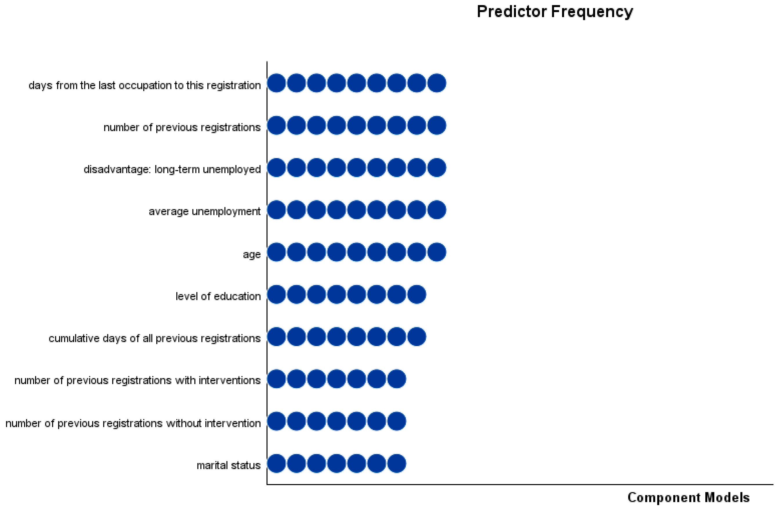
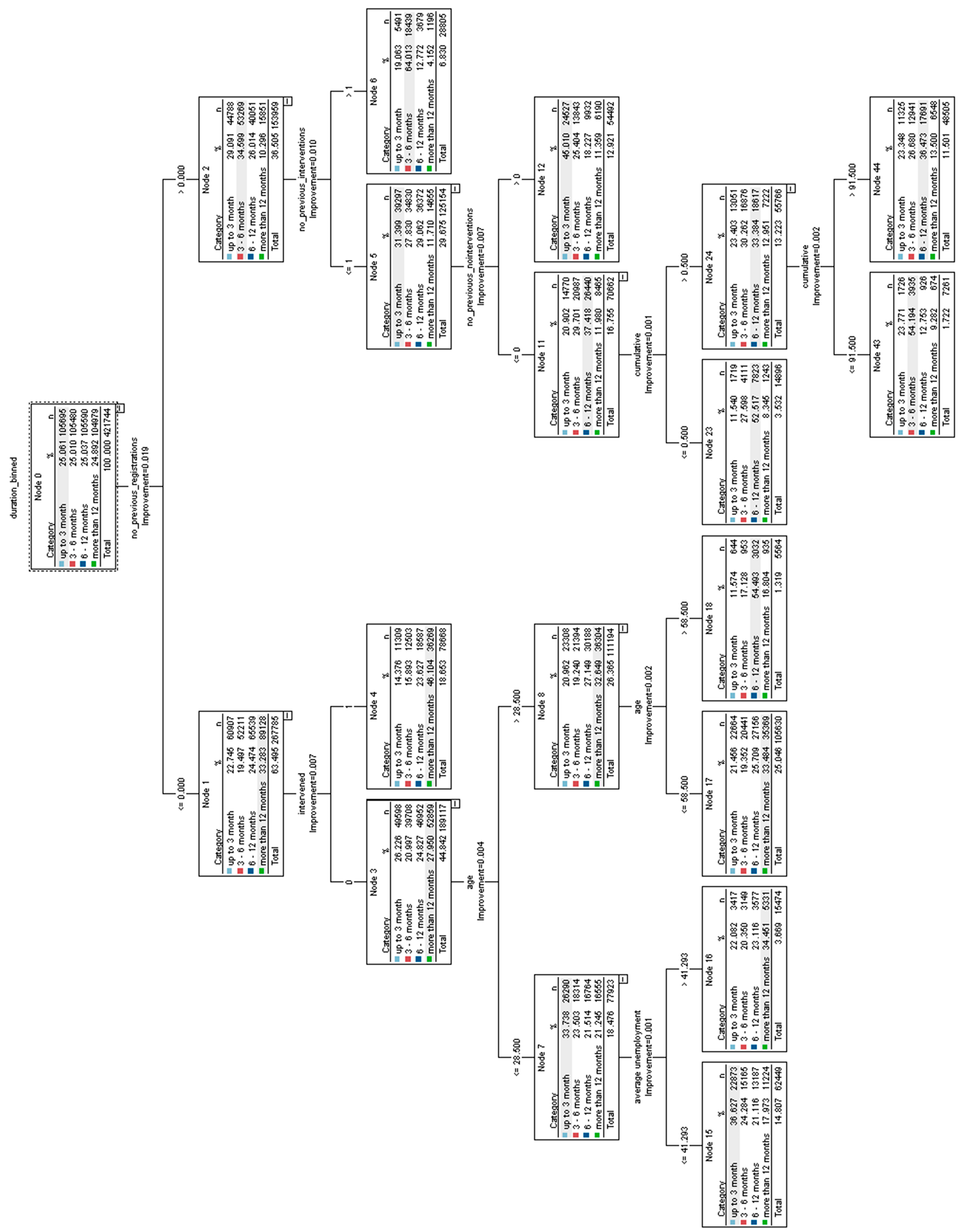
3.1. CART Model
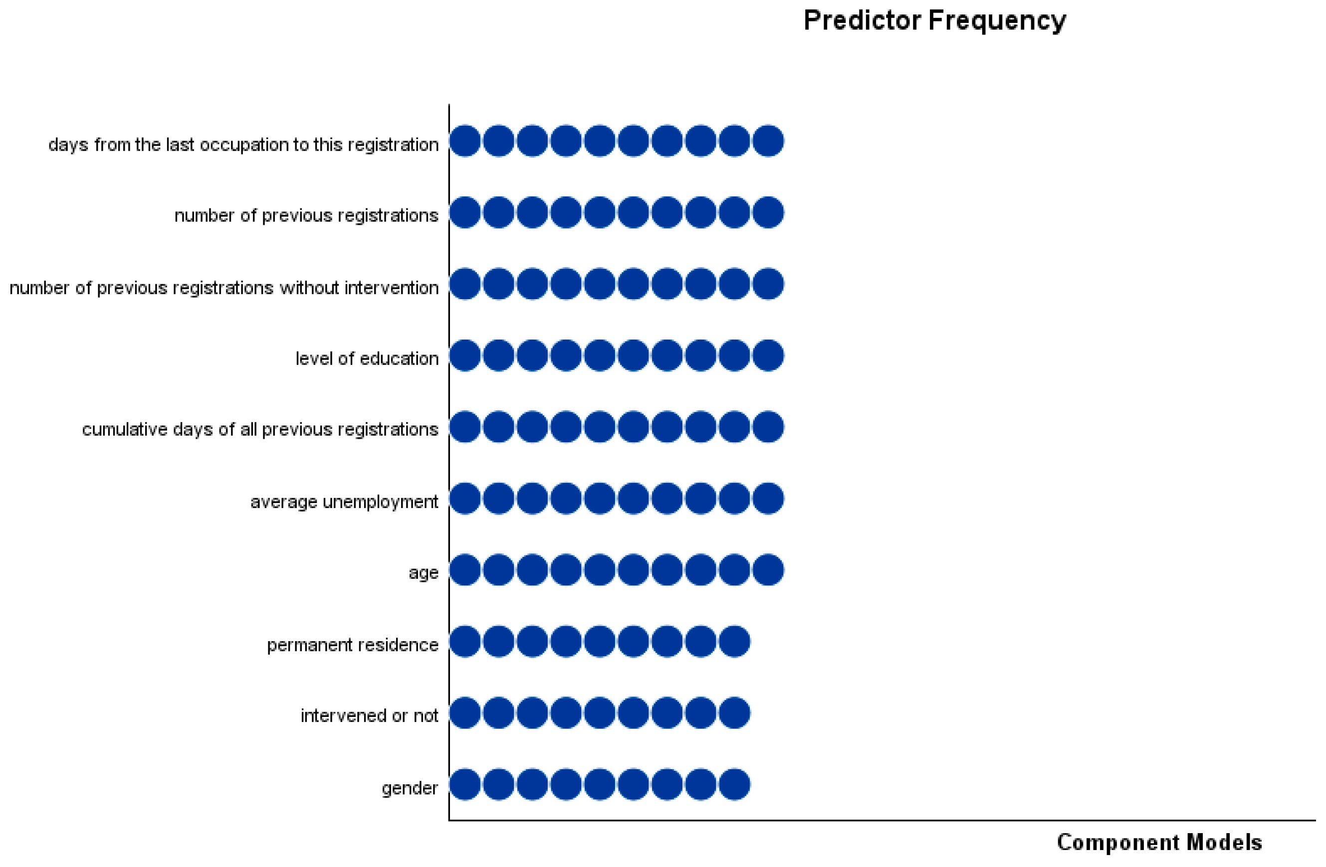
3.2. CHAID Model
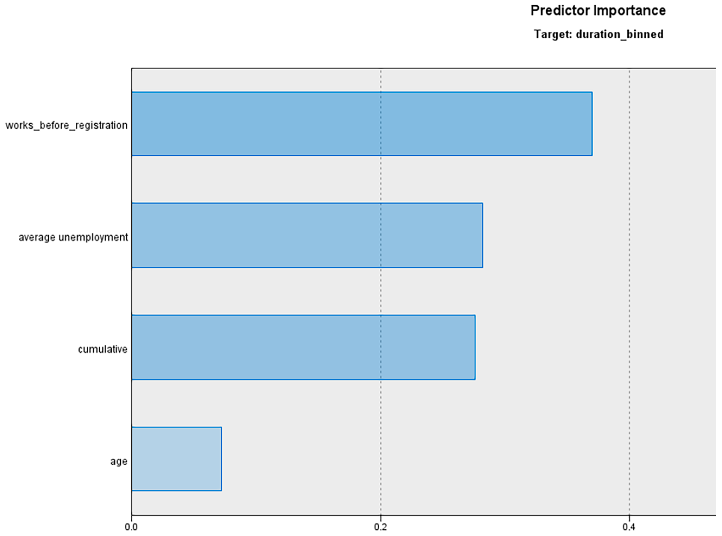
3.3. Discriminant Model
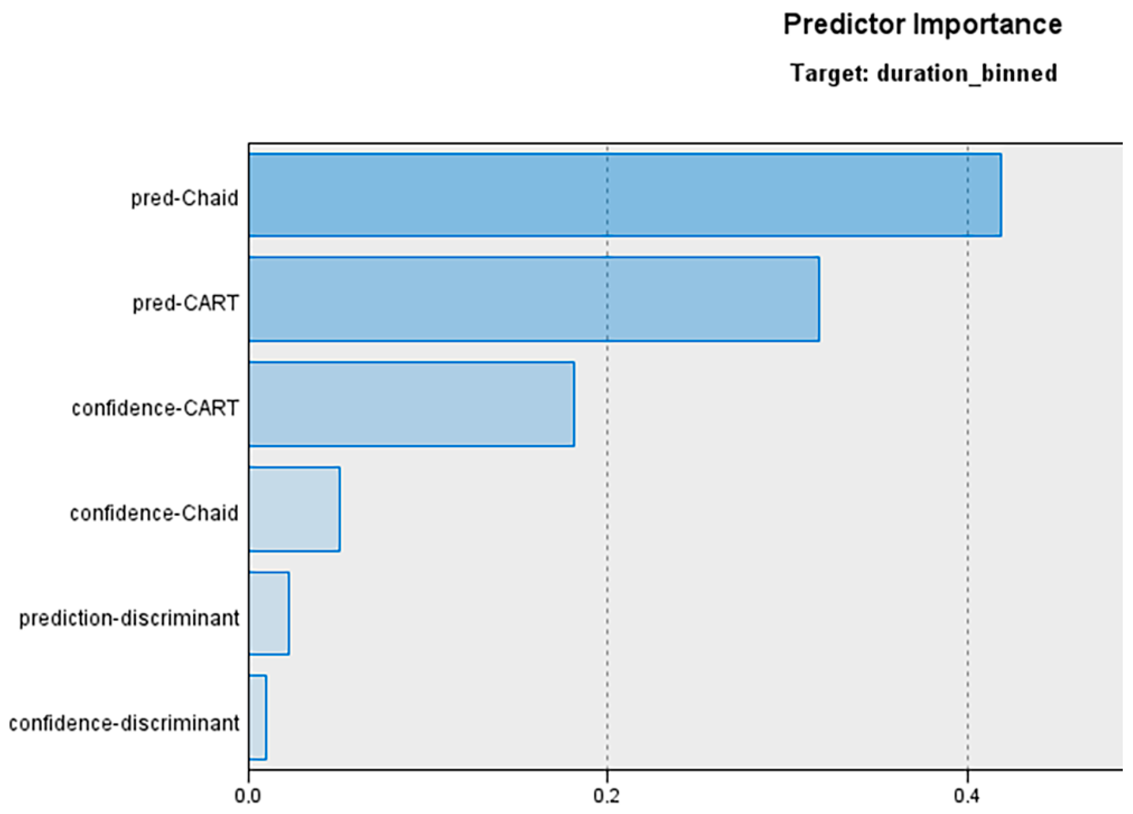
3.4. Logistic Regression Meta-Model
4. Discussion
5. Conclusions
Author Contributions
Funding
Institutional Review Board Statement
Informed Consent Statement
Data Availability Statement
Acknowledgments
Conflicts of Interest
Appendix A. Dendrogram of the CART Model

Appendix B. CART Model in Rules
Appendix C. CHAID Model in Rules
References
- Achdut, N.; Refaeli, T. Unemployment and Psychological Distress among Young People during the COVID-19 Pandemic: Psychological Resources and Risk Factors. Int. J. Environ. Res. Public Health 2020, 17, 7163. [Google Scholar] [CrossRef] [PubMed]
- Bennett, P.; Ouazad, A. Job Displacement, Unemployment, and Crime: Evidence from Danish Microdata and Reforms. J. Eur. Econ. Assoc. 2020, 18, 2182–2220. [Google Scholar] [CrossRef]
- Calmfors, L. Labour Market Policy and Unemployment. Eur. Econ. Rev. 1995, 39, 583–592. [Google Scholar] [CrossRef]
- Baliak, M.; Belin, M. The Current State of Unemployment and Its Short-Term Forecast [Aktualny Stav Nezamestnanosti a Jej Kratkodoba Prognoza]; Institute of Social Policy: Bratislava, Slovakia, 2020. [Google Scholar]
- Barcakova, M.; Janas, K. Youth Unemployment in Slovakia and in Slovenia. Izzivi Prihodnosti Chall. Future 2019, 4, 98–105. [Google Scholar]
- Caliendo, M.; Schmidl, R. Youth Unemployment and Active Labor Market Policies in Europe. IZA J. Labor Policy 2016, 5, 1. [Google Scholar] [CrossRef]
- Banociova, A.; Martinkova, S. Active Labour Market Policies of Selected European Countries and Their Competitiveness. J. Compet. 2017, 9, 5–21. [Google Scholar] [CrossRef]
- Card, D.; Kluve, J.; Weber, A. What Works? A Meta Analysis of Recent Active Labor Market Program Evaluations. J. Eur. Econ. Assoc. 2018, 16, 894–931. [Google Scholar] [CrossRef]
- Katris, C. Prediction of Unemployment Rates with Time Series and Machine Learning Techniques. Comput. Econ. 2020, 55, 673–706. [Google Scholar] [CrossRef]
- Viljanen, M.; Pahikkala, T. Predicting Unemployment with Machine Learning Based on Registry Data. In Research Challenges in Information Science; Springer International Publishing: Berlin, Germany, 2020; pp. 352–368. ISBN 978-3-030-50315-4. [Google Scholar]
- Niyadurupola, V.; Esposito, L. What Gets Them Going? The Effects of Activation Policies on Personal Change Processes of Unemployed Youth. J. Educ. Work 2021, 34, 590–609. [Google Scholar] [CrossRef]
- Prasasti, N.; Ohwada, H. Applicability of Machine-Learning Techniques in Predicting Customer Defection. In Proceedings of the 2014 International Symposium on Technology Management and Emerging Technologies, Bandung, Indonesia, 27–29 May 2014; pp. 157–162. [Google Scholar]
- Shinde, P.P.; Shah, S. A Review of Machine Learning and Deep Learning Applications. In Proceedings of the 2018 Fourth International Conference on Computing Communication Control and Automation (ICCUBEA), Pune, India, 16–18 August 2018; pp. 1–6. [Google Scholar]
- Kreiner, A.; Duca, J. Can Machine Learning on Economic Data Better Forecast the Unemployment Rate? Appl. Econ. Lett. 2020, 27, 1434–1437. [Google Scholar] [CrossRef]
- Werken, L.; Smit, V. Exploring the Use of Recurrent Neural Networks for Predicting Inflation and Unemployment. 2019. Available online: https://www.researchgate.net/profile/Victoria-Smit/publication/337171301_Exploring_the_Use_of_Recurrent_Neural_Networks_for_predicting_Inflation_and_Unemployment/links/5dc9bdfa299bf1a47b2ff69c/Exploring-the-Use-of-Recurrent-Neural-Networks-for-predicting-Inflation-and-Unemployment.pdf (accessed on 1 May 2023).
- Liu, X.; Li, L. Prediction of Labor Unemployment Based on Time Series Model and Neural Network Model. Comput. Intell. Neurosci. 2022, 2022, e7019078. [Google Scholar] [CrossRef] [PubMed]
- Kupets, O. Determinants of Unemployment Duration in Ukraine. J. Comp. Econ. 2006, 34, 228–247. [Google Scholar] [CrossRef]
- Arslan, H.; Senturk, I. Individual Determinants of Unemployment Duration in Turkey. 2018. Available online: https://hdl.handle.net/20.500.12881/3649 (accessed on 1 May 2023).
- Niragire, F.; Nshimyiryo, A. Determinants of Increasing Duration of First Unemployment among First Degree Holders in Rwanda: A Logistic Regression Analysis. J. Educ. Work. 2017, 30, 235–248. [Google Scholar] [CrossRef]
- Lim, H.-E. Predicting Low Employability Graduates: The Case of Universiti Utara Malaysia. Singap. Econ. Rev. 2010, 55, 523–535. [Google Scholar] [CrossRef]
- Bayrak, R.; Tatli, H. The Determinants of Youth Unemployment: A Panel Data Analysis of OECD Countries. Eur. J. Comp. Econ. 2018, 15, 231–248. [Google Scholar] [CrossRef]
- Logarusic, M.; Kristic, I.R. Determinants of Unemployment in the European Union. Ekon. Pregl. 2019, 70, 575–602. [Google Scholar]
- Bal-Domańska, B. The Impact of Macroeconomic and Structural Factors on the Unemployment of Young Women and Men. Econ. Change Restruct. 2022, 55, 1141–1172. [Google Scholar] [CrossRef]
- Gogas, P.; Papadimitriou, T.; Sofianos, E. Forecasting Unemployment in the Euro Area with Machine Learning. J. Forecast. 2022, 41, 551–566. [Google Scholar] [CrossRef]
- Gong, J.; Lee, C.-T. Research on Unemployment Rate Based on Machine Learning Method: A Case Study of United States from 1976 to 1986. In Proceedings of the International Conference on Cyber Security, Artificial Intelligence, and Digital Economy (CSAIDE 2022), Huzhou, China, 15–17 April 2022; Volume 12330, pp. 282–296. [Google Scholar]
- Kaya, C.; Bishop, M.; Torres, A. The Impact of Work Incentives Benefits Counseling on Employment Outcomes: A National Vocational Rehabilitation Study. J. Occup. Rehabil. 2023. [Google Scholar] [CrossRef]
- McMahon, B.T.; Hurley, J.E.; Chan, F.; Rumrill, P.D.; Roessler, R. Drivers of Hiring Discrimination for Individuals with Disabilities. J. Occup. Rehabil. 2008, 18, 133–139. [Google Scholar] [CrossRef]
- Ho, T.-W. Forecasting Unemployment via Machine Learning: The Use of Average Windows Forecasts. 2022. Available online: https://ssrn.com/abstract=3496138 (accessed on 1 July 2023).
- Papik, M.; Mihalova, P.; Papikova, L. Determinants of Youth Unemployment Rate: Case of Slovakia. Equilibrium. Q. J. Econ. Econ. Policy 2022, 17, 391–414. [Google Scholar] [CrossRef]
- Karsay, A. Structural and Cyclical Drivers of Unemployment Rate. NBS Work. Pap. 2020, 1, 1–12. [Google Scholar]
- Rublikova, E.; Lubyova, M. Estimating ARIMA–ARCH Model Rate of Unemployment in Slovakia. Progn. Pract. 2013, 5, 275–289. [Google Scholar]
- Maas, B. Short-Term Forecasting of the US Unemployment Rate. J. Forecast. 2020, 39, 394–411. [Google Scholar] [CrossRef]
- Vicente, M.R.; Lopez-Menendez, A.J.; Perez, R. Forecasting Unemployment with Internet Search Data: Does It Help to Improve Predictions When Job Destruction Is Skyrocketing? Technol. Forecast. Soc. Change 2015, 92, 132–139. [Google Scholar] [CrossRef]
- Yi, D.; Ning, S.; Chang, C.-J.; Kou, S.C. Forecasting Unemployment Using Internet Search Data via PRISM. J. Am. Stat. Assoc. 2021, 116, 1662–1673. [Google Scholar] [CrossRef]
- Ganaie, M.A.; Hu, M.; Malik, A.K.; Tanveer, M.; Suganthan, P.N. Ensemble Deep Learning: A Review. Eng. Appl. Artif. Intell. 2022, 115, 105151. [Google Scholar] [CrossRef]
- Parker, W.S. Ensemble Modeling, Uncertainty and Robust Predictions. WIREs Clim. Change 2013, 4, 213–223. [Google Scholar] [CrossRef]
- Kotsiantis, S.B.; Pintelas, P.E. Combining Bagging and Boosting. Int. J. Math. Comput. Sci. 2007, 1, 372–381. [Google Scholar]
- Kotsiantis, S.B. Supervised Machine Learning: A Review of Classification Techniques. Informatica 2007, 31, 249–268. [Google Scholar]
- Adamko, P.; Siekelova, A. An Ensemble Model for Prediction of Crisis in Slovak Companies. In Proceedings of the 17th International Scientific Conference Globalization and Its Socio-Economic Consequences: Proceedings, Rajecke Teplice, Slovakia, 4–5 October 2017; University of Zilina: Zilina, Slovakia, 2017. Part I. pp. 1–7. [Google Scholar]
- Kim, M.-J.; Kang, D.-K. Ensemble with Neural Networks for Bankruptcy Prediction. Expert Syst. Appl. 2010, 37, 3373–3379. [Google Scholar] [CrossRef]
- Pavlicko, M.; Durica, M.; Mazanec, J. Ensemble Model of the Financial Distress Prediction in Visegrad Group Countries. Mathematics 2021, 9, 1886. [Google Scholar] [CrossRef]
- Bhagia, D. Duration Dependence and Heterogeneity: Learning from Early Notice of Layoff. arXiv 2023, arXiv:2305.17344. [Google Scholar]
- Mueller, A.I.; Spinnewijn, J. The Nature of Long-Term Unemployment: Predictability, Heterogeneity and Selection. IZA Discuss. Pap. Ser. 2023, 15955, 1–41. [Google Scholar]
- Song, Y.; Lu, Y. Decision Tree Methods: Applications for Classification and Prediction. Shanghai Arch. Psychiatry 2015, 27, 130–135. [Google Scholar] [CrossRef] [PubMed]
- Breiman, L.; Friedman, J.H.; Olshen, R.A.; Stone, C.J. Classification and Regression Trees; The Wadsworth statistics/probability series; Wadsworth & Brooks/Cole Advanced Books & Software: Monterey, CA, USA, 1984; ISBN 978-1-351-46048-4. [Google Scholar]
- Rutkowski, L.; Jaworski, M.; Pietruczuk, L.; Duda, P. The CART Decision Tree for Mining Data Streams. Inf. Sci. 2014, 266, 1–15. [Google Scholar] [CrossRef]
- Priyam, A.; Gupta, R.; Rathee, A.; Srivastava, S. Comparative Analysis of Decision Tree Classification Algorithms. Int. J. Curr. Eng. Technol. 2013, 3, 334–337. [Google Scholar]
- Ozcan, M.; Peker, S. A Classification and Regression Tree Algorithm for Heart Disease Modeling and Prediction. Healthc. Anal. 2023, 3, 100130. [Google Scholar] [CrossRef]
- Kass, G.V. An Exploratory Technique for Investigating Large Quantities of Categorical Data. J. R. Stat. Society. Ser. C Appl. Stat. 1980, 29, 119–127. [Google Scholar] [CrossRef]
- Milanovic, M.; Stamenkovic, M. CHAID Decision Tree: Methodological Frame and Application. Econ. Themes 2016, 54, 563–586. [Google Scholar] [CrossRef]
- Ritschard, G. CHAID and Earlier Supervised Tree Methods. In Contemporary Issues in Exploratory Data Mining in Behavioral Sciences; McArdle, J.J., Ritschard, G., Eds.; Routeledge: New York, NY, USA, 2013; pp. 48–74. [Google Scholar]
- McLachlan, G.J. Discriminant Analysis and Statistical Pattern Recognition; John Wiley & Sons: Hoboken, NJ, USA, 2004; ISBN 978-0-471-69115-0. [Google Scholar]
- Fisher, R.A. The Use of Multiple Measurements in Taxonomic Problems. Ann. Eugen. 1936, 7, 179–188. [Google Scholar] [CrossRef]
- Bickel, P.J.; Levina, E. Some Theory for Fisher’s Linear Discriminant Function, “Naive Bayes”, and Some Alternatives When There Are Many More Variables than Observations. Bernoulli 2004, 10, 989–1010. [Google Scholar] [CrossRef]
- Tabachnick, B.G.; Fidell, L.S.; Ullman, J.B. Using Multivariate Statistic, 7th ed.; Pearson: New York, NY, USA, 2019; ISBN 978-0-13-479054-1. [Google Scholar]
- Gajdosikova, D.; Lăzăroiu, G.; Valaskova, K. How Particular Firm-Specific Features Influence Corporate Debt Level: A Case Study of Slovak Enterprises. Axioms 2023, 12, 183. [Google Scholar] [CrossRef]
- Hosmer, D.W., Jr.; Lemeshow, S.; Sturdivant, R.X. Applied Logistic Regression, 3rd ed.; Wiley: New York, NY, USA, 2013; ISBN 978-0-470-58247-3. [Google Scholar]
- Agresti, A. Foundations of Linear and Generalized Linear Models, 2nd ed.; Wiley: New York, NY, USA, 2015; ISBN 978-1-118-73003-4. [Google Scholar]
- Act No. 5/2004 Coll. on Employment Services and on Amending Certain Laws; Ministry of Labour, Social Affairs and Family, Slovakia: Bratislava, Slovakia, 2004; Volume 2004.
- Brownlee, J. Classification Accuracy Is Not Enough: More Performance Measures You Can Use; Machine Learning Mastery: San Juan, PR, USA, 2014. [Google Scholar]
- Kroft, K.; Lange, F.; Notowidigdo, M.J. Duration Dependence and Labor Market Conditions: Evidence from a Field Experiment. Q. J. Econ. 2013, 128, 1123–1167. [Google Scholar] [CrossRef]
- Babos, P.; Lubyova, M. Effect of Labour Code Reform on Unemployment Duration in the Course of Crisis: Evidence from Slovakia. Ekon. Cas. 2016, 64, 218–237. [Google Scholar]
- Lachiheb, A.B.A. Intermediation and Decision Support System for the Management of Unemployment: The Simulator of Duration. In Proceedings of the Digital Economy. Emerging Technologies and Business Innovation, Sidi Bou Said, Tunisia, 4–6 May 2017; Jallouli, R., Zaiane, O.R., Bach Tobji, M.A., Srarfi Tabbane, R., Nijholt, A., Eds.; Springer International Publishing: Cham, Switzerland, 2017; pp. 105–115. [Google Scholar]
- Marksoo, U.; Tammaru, T. Long-Term Unemployment in Economic Boom and Bust: The Case of Estonia. Trames 2011, 15, 215. [Google Scholar] [CrossRef]


| Variable | Description | Values | Proportion |
|---|---|---|---|
| gender | gender of jobseeker | male | 52.26% |
| female | 47.74% | ||
| nationality | nationality of jobseeker | Slovak | 89.31% |
| Hungarian | 9.35% | ||
| unknown or other | 0.80% | ||
| Czech | 0.37% | ||
| Roma | 0.16% | ||
| marital status | marital status of jobseeker | single | 51.51% |
| married | 37.21% | ||
| divorced | 9.36% | ||
| widow | 1.50% | ||
| unknown | 0.42% | ||
| permanent residence | permanent residence of the jobseeker (part of Slovakia) | Eastern Slovakia | 33.79% |
| Western Slovakia | 32.13% | ||
| Central Slovakia | 26.72% | ||
| Bratislava region | 7.36% | ||
| education | highest achieved education of the jobseeker | non-finished primary | 28.32% |
| primary | 30.03% | ||
| lower secondary vocational | 13.04% | ||
| secondary vocational | 5.16% | ||
| complete secondary | 0.72% | ||
| general secondary | 0.17% | ||
| higher vocational | 8.86% | ||
| university 1st | 0.57% | ||
| university 2nd | 2.55% | ||
| university 3rd | 9.25% | ||
| NA | 1.31% | ||
| disadvantage: school leaver | disadvantaged jobseeker | no | 84.53% |
| yes | 15.47% | ||
| disadvantage: over 50 years | disadvantaged jobseeker | no | 84.08% |
| yes | 15.92% | ||
| disadvantage: long-term unemployed | disadvantaged jobseeker | no | 68.18% |
| yes | 31.82% | ||
| disadvantage: health | disadvantaged jobseeker | no | 97.13% |
| yes | 2.87% | ||
| disadvantage: no paid job | disadvantaged jobseeker | no | 55.60% |
| yes | 44.40% | ||
| disadvantage: low education | disadvantaged jobseeker | no | 86.19% |
| yes | 13.81% | ||
| disadvantage: organisational reasons | disadvantaged jobseeker | no | 99.58% |
| yes | 0.42% | ||
| disadvantage: others | disadvantaged jobseeker | no | 99.70% |
| Yes | 0.30% | ||
| children | number of children of the jobseeker | 0 | 87.78% |
| 1 | 6.57% | ||
| 2 | 3.85% | ||
| 3 | 1.16% | ||
| 4 or more | 0.64% | ||
| reason of exclusion | reason of exclusion from the database of jobseekers | employment | 54.25% |
| relevant reason of exclusion | 34.78% | ||
| non-co-operation | 10.97% | ||
| intervention | intervened jobseeker | No | 65.95% |
| Yes | 34.05% | ||
| previous registrations | number of all previous registrations | 0 | 64.94% |
| 1 | 22.51% | ||
| 2 | 7.02% | ||
| 3 | 2.47% | ||
| 4 | 1.11% | ||
| 5 or more | 1.95% | ||
| previous non-interventions | number of previous registrations without intervention | 0 | 87.54% |
| 1 | 10.25% | ||
| 2 | 1.79% | ||
| 3 or more | 0.42% | ||
| previous interventions | number of previous registrations with intervention | 0 | 87.81% |
| 1 | 6.03% | ||
| 2 | 2.29% | ||
| 3 | 1.21% | ||
| 4 or more | 2.67% |
| Variable | Description | Mean | Min | Max | Range | Std. Deviation | Median | Mode |
|---|---|---|---|---|---|---|---|---|
| age | age of jobseeker at the beginning of registration | 34.9 | 15.0 | 78.0 | 63.0 | 12.5 | 32.0 | 24.0 |
| cumulative previous registrations | cumulative number of days of previous registrations before the period under review | 1155.1 | 0.0 | 33,722.0 | 33,722.0 | 1343.8 | 699.0 | 0.0 |
| work before registration | number of days from the last occupation to the current registration | 414.7 | 0.0 | 15,805.0 | 15,805.0 | 1068.4 | 1.0 | 0.0 |
| average unemployment | average number of days spent in unemployment per year from 15 years of age | 45.07 | 0.0 | 364.94 | 364.94 | 54.2 | 26.1 | 0.0 |
| duration of registration | duration of the current registration in days | 300.9 | 0.0 | 1365.0 | 1365.0 | 303.8 | 182.0 | 91.0 |
| Duration of Registration | Proportion of the Sample | Multiplication Factor for Balancing via Boosting |
|---|---|---|
| up to 3 months | 23.85% | 1.2036 |
| 3–6 months | 21.34% | 1.3453 |
| 6–12 months | 26.10% | 1.0998 |
| more than 12 months | 28.71% | 1.0000 |
| Unemployment Duration | Up to 3 Months | 3–6 Months | 6–12 Months | More than 12 Months | Sum | Correct [%] |
|---|---|---|---|---|---|---|
| up to 3 months | 86,484 | 10,519 | 25,631 | 2391 | 125,025 | 0.692 |
| 3–6 months | 54,710 | 25,734 | 29,698 | 1890 | 112,032 | 0.230 |
| 6–12 months | 64,445 | 8266 | 60,991 | 2974 | 136,676 | 0.446 |
| more than 12 months | 11,136 | 2691 | 22,551 | 114,202 | 150,580 | 0.758 |
| sum | 216,775 | 47,210 | 138,871 | 121,457 | 524,313 | 0.548 |
| Unemployment Duration | Sum Correct | Sum Incorrect | Sum | Correct [%] |
|---|---|---|---|---|
| sum correct | 287,411 | 236,902 | 524,313 | 54.82 |
| sum incorrect | 236,902 | 1,336,037 | 1,572,939 | 84.94 |
| sum | 524,313 | 1,572,939 | 2,097,252 | 77.41 |
| correct [%] | 54.82 | 15.06 |
| Evaluation Measure | Up to 3 Months | 3–6 Months | 6–12 Months | More than 12 Months | Macro-Average | Micro-Average |
|---|---|---|---|---|---|---|
| sensitivity | 69.17 | 22.97 | 44.62 | 75.84 | 53.15 | 54.82 |
| specificity | 67.37 | 94.79 | 79.91 | 98.06 | 85.03 | 84.94 |
| precision | 39.90 | 54.51 | 43.92 | 94.03 | 58.09 | 54.82 |
| F-measure | 50.61 | 32.32 | 44.27 | 83.96 | 52.79 | 54.82 |
| accuracy | 39.90 | 79.44 | 70.71 | 91.68 | 77.41 | 77.41 |
| Unemployment Duration | Up to 3 Months | 3–6 Months | 6–12 Months | More than 12 Months | Sum | Correct [%] |
|---|---|---|---|---|---|---|
| up to 3 months | 52,351 | 20,851 | 22,556 | 29,267 | 125,025 | 0.419 |
| 3–6 months | 30,143 | 35,092 | 22,129 | 24,668 | 112,032 | 0.313 |
| 6–12 months | 33,378 | 20,786 | 42,928 | 39,584 | 136,676 | 0.314 |
| more than 12 months | 30,784 | 16,771 | 26,399 | 76,626 | 150,580 | 0.509 |
| sum | 146,656 | 93,500 | 114,012 | 170,145 | 524,313 | 0.395 |
| Unemployment Duration | Sum Correct | Sum Incorrect | Sum | Correct [%] |
|---|---|---|---|---|
| sum correct | 206,997 | 317,316 | 524,313 | 39.48 |
| sum incorrect | 317,316 | 1,255,623 | 1,572,939 | 79.83 |
| sum | 524,313 | 1,572,939 | 2,097,252 | 69.74 |
| correct [%] | 39.48 | 20.17 |
| Evaluation Measure | Up to 3 Months | 3–6 Months | 6–12 Months | More than 12 Months | Macro-Average | Micro-Average |
|---|---|---|---|---|---|---|
| sensitivity | 41.87 | 31.32 | 31.41 | 50.89 | 38.87 | 39.48 |
| specificity | 76.38 | 85.83 | 81.66 | 74.98 | 79.71 | 79.83 |
| precision | 35.70 | 37.53 | 37.65 | 45.04 | 38.98 | 39.48 |
| F-measure | 38.54 | 34.15 | 34.25 | 47.78 | 38.68 | 56.60 |
| accuracy | 35.70 | 74.19 | 68.56 | 68.06 | 69.74 | 69.74 |
| Function | Up to 3 Months | 3–6 Months | 6–12 Months |
|---|---|---|---|
| age | −0.086 (−0.135) | 0.612 (0.723) | 0.149 (−0.062) |
| work before registration | 0.289 (0.113) | 0.488 (0.708) | −0.718 (−0.562) |
| cumulative previous registrations | 0.734 (0.723) | 0.298 (0.239) | 0.610 (0.612) |
| average unemployment | −0.692 (−0.614) | 0.306 (0.460) | 0.552 (0.422) |
| Unemployment Duration | Up to 3 Months | 3–6 Months | 6–12 Months | More than 12 Months | Sum | Correct [%] |
|---|---|---|---|---|---|---|
| up to 3 months | 80,095 | 11,131 | 7651 | 26,148 | 125,025 | 0.641 |
| 3–6 months | 58,857 | 20,914 | 7879 | 24,382 | 112,032 | 0.187 |
| 6–12 months | 71,058 | 15,161 | 10,756 | 39,701 | 136,676 | 0.079 |
| more than 12 months | 71,596 | 12,336 | 7016 | 59,632 | 150,580 | 0.396 |
| sum | 281,606 | 59,542 | 33,302 | 149,863 | 524,313 | 0.327 |
| Unemployment Duration | Sum Correct | Sum Incorrect | Sum | Correct [%] |
|---|---|---|---|---|
| sum correct | 171,397 | 352,916 | 524,313 | 32.69 |
| sum incorrect | 352,916 | 1,220,023 | 1,572,939 | 77.56 |
| sum | 524,313 | 1,572,939 | 2,097,252 | 66.34 |
| correct [%] | 32.69 | 22.44 |
| Evaluation Measure | Up to 3 Months | 3–6 Months | 6–12 Months | More than 12 Months | Macro-Average | Micro-Average |
|---|---|---|---|---|---|---|
| sensitivity | 64.06 | 18.67 | 7.87 | 39.60 | 32.55 | 32.69 |
| specificity | 49.53 | 90.63 | 94.18 | 75.86 | 77.55 | 77.56 |
| precision | 28.44 | 35.12 | 32.30 | 39.79 | 33.91 | 32.69 |
| F-measure | 39.39 | 24.38 | 12.66 | 39.70 | 29.03 | 32.69 |
| accuracy | 28.44 | 75.25 | 71.68 | 65.44 | 66.34 | 66.34 |
| Unemployment Duration | Up to 3 Months | 3–6 Months | 6–12 Months | More than 12 Months |
|---|---|---|---|---|
| age | 0.227 | 0.242 | 0.240 | 0.240 |
| work before registration | −0.001 | 0.0004 | 0.0005 | −0.001 |
| cumulative | 0.002 | 0.003 | 0.002 | 0.002 |
| average unemployment | 0.011 | 0.012 | 0.014 | 0.018 |
| (constant) | −50.520 | −60.201 | −60.126 | −60.119 |
| Unemployment Duration | 3–6 Months | 6–12 Months | More than 12 Months |
|---|---|---|---|
| Intercept | −2.014 | 0.475 | −0.686 |
| pred-CART_cat1 | 0.102 | −0.738 | −1.745 |
| pred-CART_cat2 | 0.870 | −0.390 | −2.266 |
| pred-CART_cat3 | 0.425 | −0.023 | −1.361 |
| confidence-CART | 0.759 | −2.932 | 3.768 |
| pred-CHAID _cat1 | −0.074 | −0.451 | −2.591 |
| pred-CHAID _cat2 | 0.602 | −0.054 | −1.861 |
| pred-CHAID _cat3 | 0.380 | 0.336 | −1.820 |
| confidence-CHAID | 2.379 | 2.375 | 3.087 |
| pred-discriminant_cat1 | −0.035 | −0.158 | −0.263 |
| pred-discriminant_cat2 | 0.144 | −0.036 | −0.453 |
| pred-discriminant_cat3 | 0.046 | 0.196 | −0.096 |
| confidence-discriminant | 0.474 | 0.414 | 0.971 |
| Unemployment Duration | Up to 3 Months | 3–6 Months | 6–12 Months | More than 12 Months | Sum | Correct [%] |
|---|---|---|---|---|---|---|
| up to 3 months | 68,854 | 18,414 | 34,376 | 3381 | 125,025 | 0.551 |
| 3–6 months | 40,017 | 33,368 | 35,863 | 2784 | 112,032 | 0.298 |
| 6–12 months | 44,096 | 19,257 | 68,413 | 4910 | 136,676 | 0.501 |
| more than 12 months | 11,411 | 4467 | 15,962 | 118,740 | 150,580 | 0.789 |
| sum | 164,378 | 75,506 | 154,614 | 129,815 | 524,313 | 0.552 |
| Unemployment Duration | Sum Correct | Sum Incorrect | Sum | Correct [%] |
|---|---|---|---|---|
| sum correct | 289,375 | 234,938 | 524,313 | 55.19 |
| sum incorrect | 234,938 | 1,338,001 | 1,572,939 | 85.06 |
| sum | 524,313 | 1,572,939 | 2,097,252 | 77.60 |
| correct [%] | 55.19 | 14.94 |
| Evaluation Measure | Up to 3 Months | 3–6 Months | 6–12 Months | More than 12 Months | Macro-Average | Micro-Average |
|---|---|---|---|---|---|---|
| sensitivity | 55.07 | 29.78 | 50.05 | 78.86 | 53.44 | 55.19 |
| specificity | 76.08 | 89.78 | 77.76 | 97.04 | 85.16 | 85.06 |
| precision | 41.89 | 44.19 | 44.25 | 91.47 | 55.45 | 55.19 |
| F-measure | 47.58 | 35.59 | 46.97 | 84.69 | 53.71 | 55.19 |
| accuracy | 41.89 | 76.96 | 70.54 | 91.82 | 77.60 | 77.60 |
Disclaimer/Publisher’s Note: The statements, opinions and data contained in all publications are solely those of the individual author(s) and contributor(s) and not of MDPI and/or the editor(s). MDPI and/or the editor(s) disclaim responsibility for any injury to people or property resulting from any ideas, methods, instructions or products referred to in the content. |
© 2023 by the authors. Licensee MDPI, Basel, Switzerland. This article is an open access article distributed under the terms and conditions of the Creative Commons Attribution (CC BY) license (https://creativecommons.org/licenses/by/4.0/).
Share and Cite
Gabrikova, B.; Svabova, L.; Kramarova, K. Machine Learning Ensemble Modelling for Predicting Unemployment Duration. Appl. Sci. 2023, 13, 10146. https://doi.org/10.3390/app131810146
Gabrikova B, Svabova L, Kramarova K. Machine Learning Ensemble Modelling for Predicting Unemployment Duration. Applied Sciences. 2023; 13(18):10146. https://doi.org/10.3390/app131810146
Chicago/Turabian StyleGabrikova, Barbora, Lucia Svabova, and Katarina Kramarova. 2023. "Machine Learning Ensemble Modelling for Predicting Unemployment Duration" Applied Sciences 13, no. 18: 10146. https://doi.org/10.3390/app131810146