
Establishment of Localized Utilization Parameters for Numerical Simulation Analysis Applied to Deep Excavations

Abstract
:1. Introduction
1.1. Engineering Properties and Microzonation of Taipei Basin
1.2. Literature Review on Finite Element Method
1.3. Soil Elastic Modulus
1.4. Literature Review on Sensitivity Analysis of Parameters
1.5. Literature Review on Prediction of Maximum Wall Deflection
2. Materials and Methods
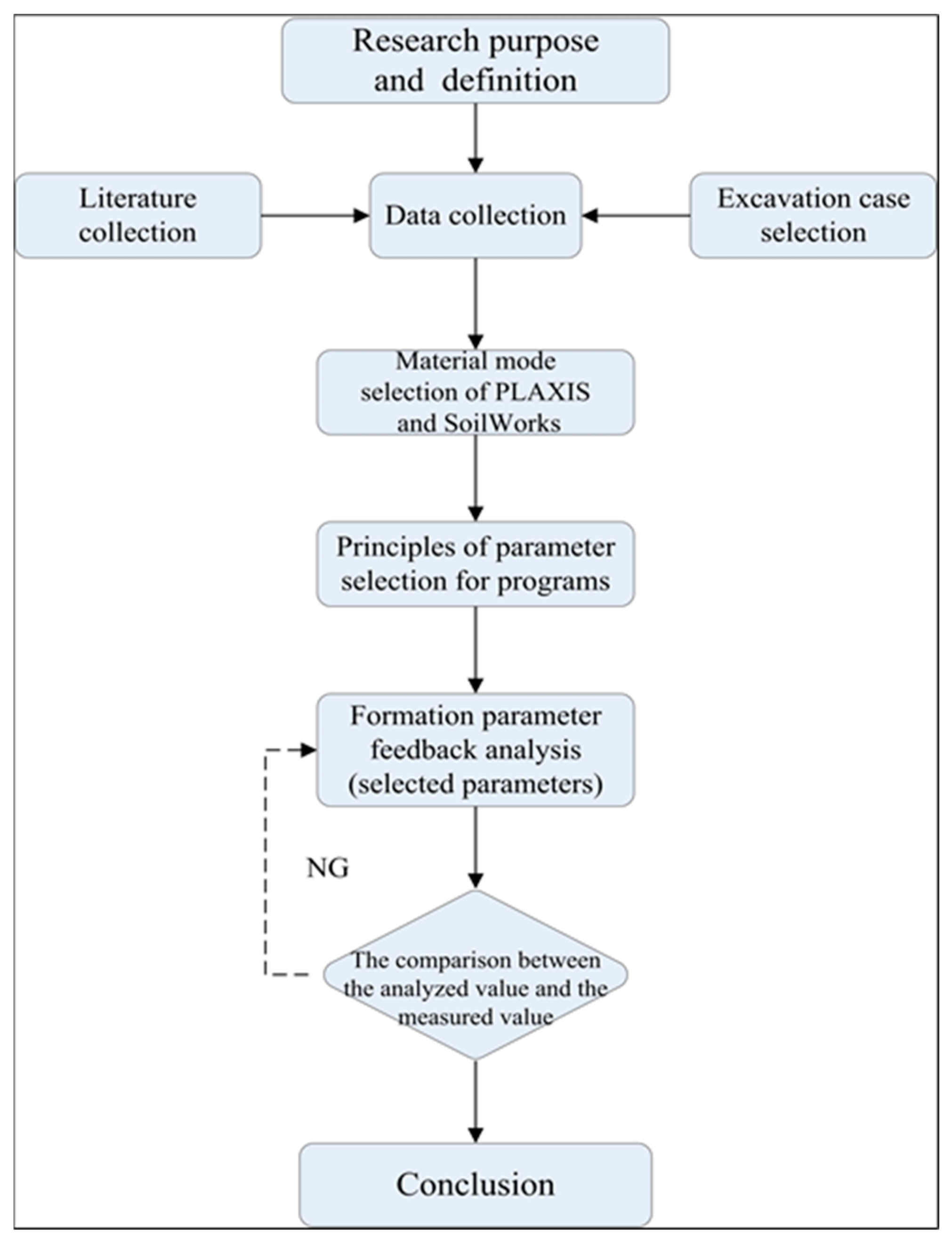
2.1. Research Method and Procedure
2.2. Research Materials
- PLAXIS Numerical SimulationThe background and characteristics of the PLAXIS program, along with an explanation of the numerical analysis model used, can be found in [4]. Case studies of gravel layer excavations in the Xindian area of New Taipei City were collected, and a feedback analysis was performed using the existing monitoring data to derive suitable soil parameters for analysis using the PLAXIS program for the gravel layers.
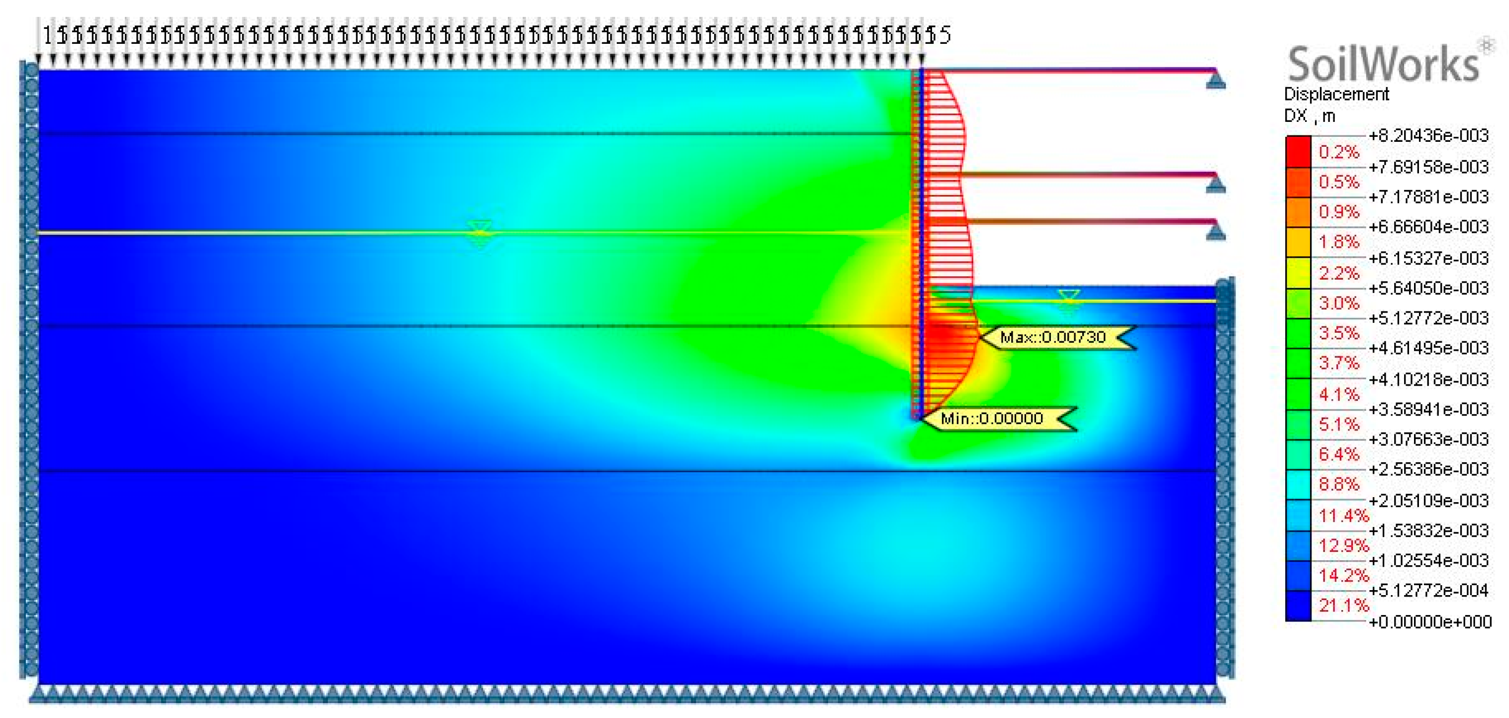
- SoilWorks Numerical SimulationThe background and characteristics of the SoilWorks program can be found in [34]. A sensitivity analysis was conducted using the basic case model and variations in the soil parameters adopted in previous studies, comparing the results with previous PLAXIS outcomes. The case study of gravel layer excavation in the Xindian area mentioned in the previous section was utilized to derive suitable soil parameters for analysis using the SoilWorks program. An additional case study, Case 3, was included for parameter verification.
3. PLAXIS Numerical Simulation
3.1. Analysis Methods and Models
Parameter Configuration and Modeling for Numerical Simulation Analysis
- Parameter Configuration
- (1)
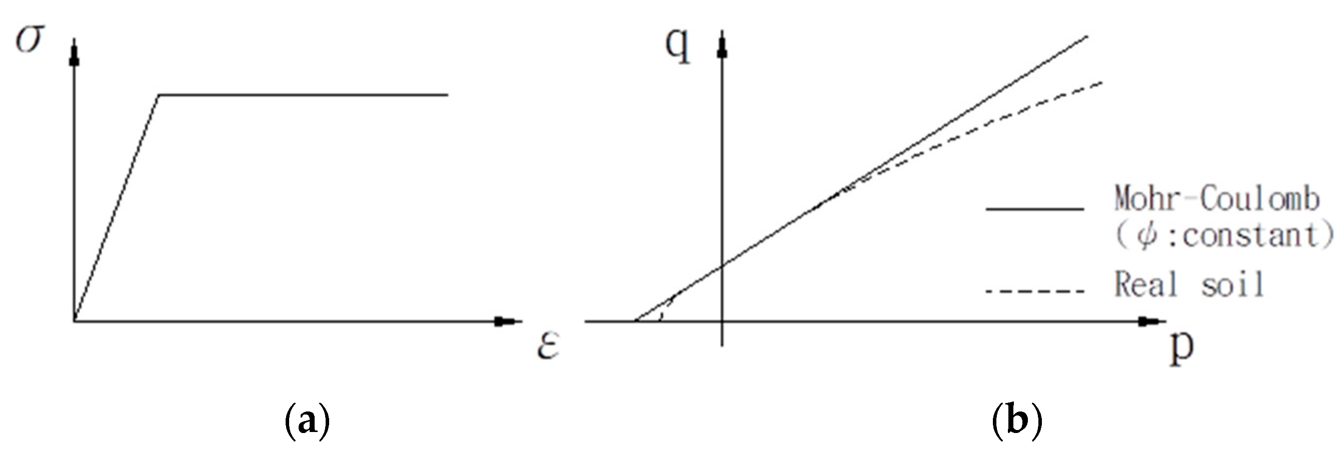
- Soil Parameters: In this study, the Mohr–Coulomb model, which is a built-in model within PLAXIS, was selected to simulate the soil behavior. The Mohr–Coulomb model is an elastic–perfectly plastic failure model based on elastoplastic theory. It considers factors such as the satisfaction of Hook’s Law during the elastic stage, yielding criteria, and the flow rule. The soil parameters required for this model are explained as follows:
- Elastic modulus (Es): In general, the soil can be assigned an elastic modulus of 50% of the ultimate strength, known as the secant modulus (E50).
- Poisson’s ratio (ν): In most cases, the value of ν for soils ranges between 0.3 and 0.4.
- Cohesion (c): According to the PLAXIS user manual, a value of c greater than 0.2 kPa can be input for computational convenience.
- Internal friction angle (Φ): The internal friction angle of the soil can be determined based on the soil type and shear strength tests conducted in the field or laboratory.
- Dilation angle (ψ): For cohesive soils, the dilation angle can be assumed to be 0. In the case of sandy soils, the angle is very small and sometimes even close to zero or negative (ψ ≒ 0° or ψ < 0°); therefore, it can be assumed as ψ = 0° during the analysis.
- (2)
- Retaining Structure Parameters
- Boundary Conditions for Numerical Analysis Modeling
3.2. Case Analysis
3.2.1. Case Study 1
- Site DescriptionThe site is located on the south side of Minquan Road, Xindian District, New Taipei City, with an area of approximately 8522 m2. The site has an irregular shape, and the terrain varies within 1 m (Geotechnical Engineering Co., Ltd., New Taipei City, Taiwan. [42]).
- Subsurface StrataThe subsurface strata at the site can be simplified into five layers from top to bottom, as described by Lin [43] and Geotechnical Engineering Co., Ltd. [44]. The simplified engineering parameters of the strata are shown in Table A1. The groundwater level at the site is approximately 10.7 to 11.3 m below the ground surface, and the groundwater pressure in the fifth layer of gravel is around 11.4 to 11.6 m below the ground surface, which is close to the free water level. For analysis purposes, the initial groundwater level is set at 11 m below the ground surface.
- Foundation Excavation Planning
- (1)
- Geotechnical facilities: The foundation excavation has a depth of 17.30 m and utilizes a raft foundation. The retaining structure consists of a continuous wall with a thickness of 70 cm, and the wall depth is 27 m.
- (2)
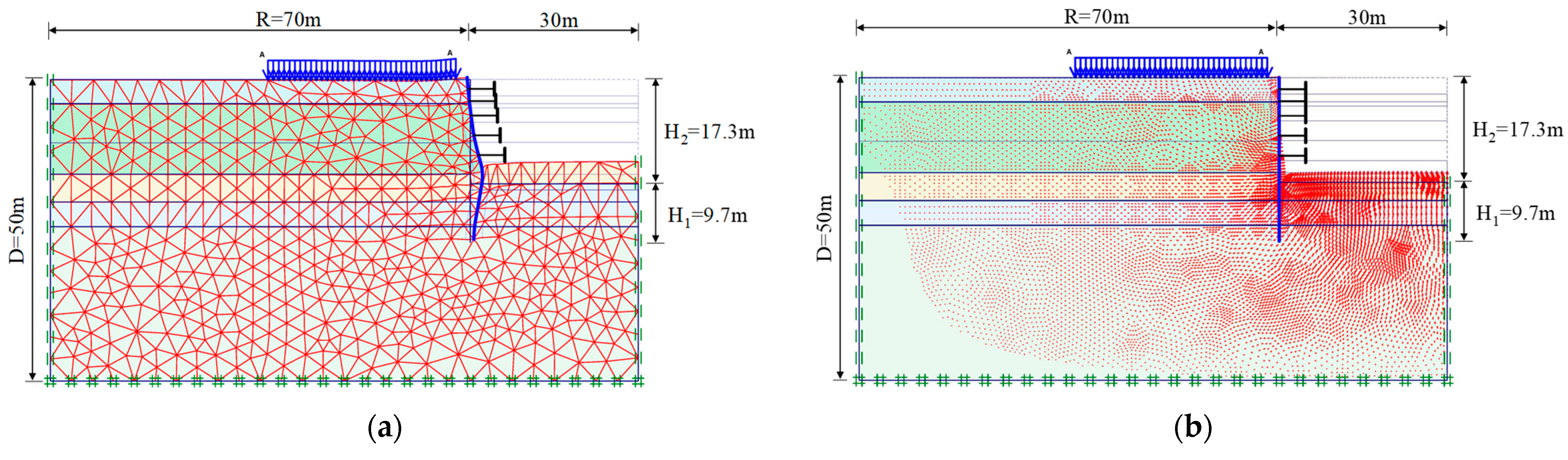
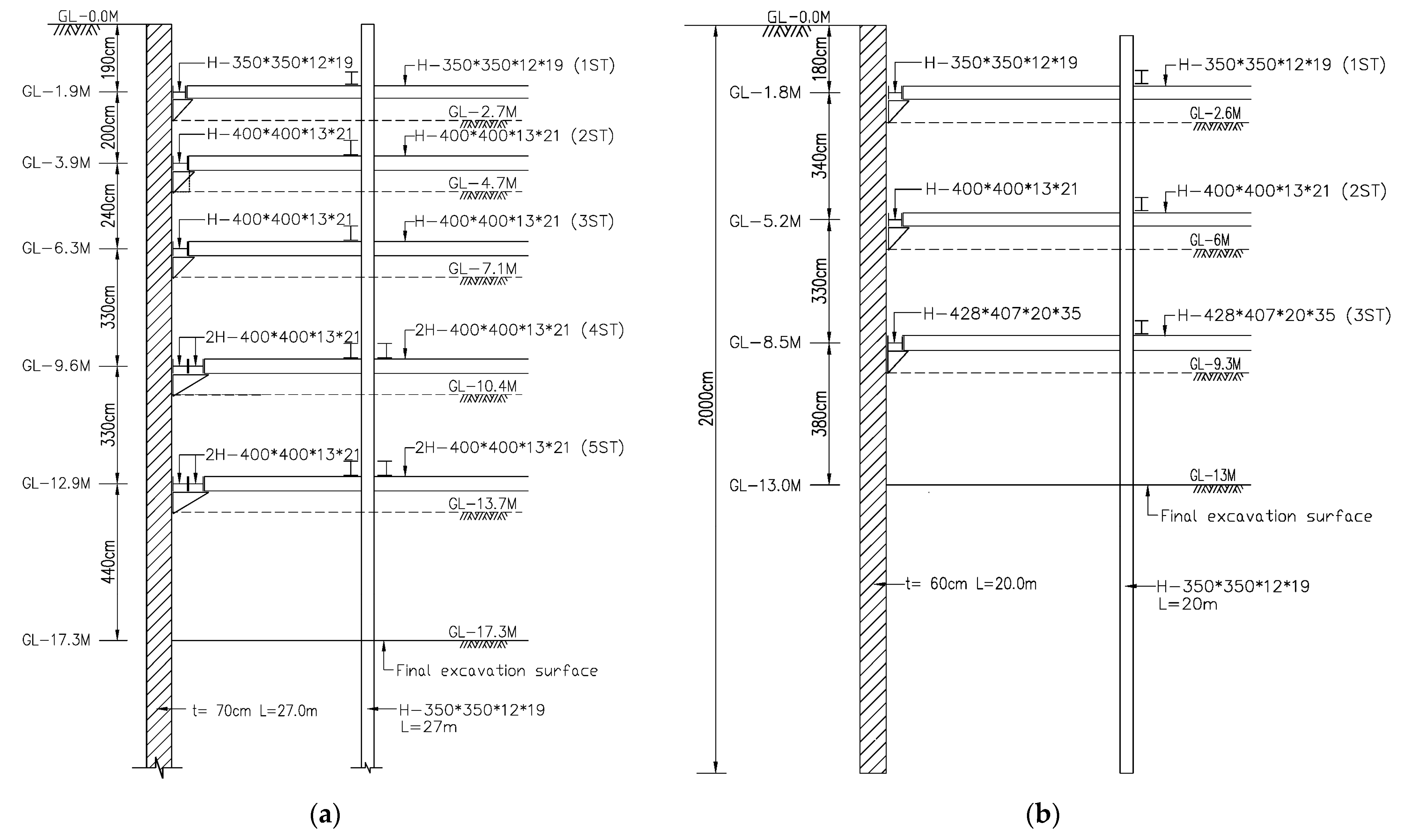
- Internal bracing system: The excavation follows a top-down sequence with staged excavation and horizontal bracing. The bracing system consists of five levels, using H-beams as support structures. The excavation profile is shown in Figure A1a.
- (3)
- Excavation steps: The first stage involves excavation to GL.−2.7 m, followed by the installation of the first-level bracing. The second stage involves excavation to GL.−4.7 m and the installation of the second-level bracing. The third stage involves excavation to GL.−7.1 m and the installation of the third-level bracing. The fourth stage involves excavation to GL.−10.4 m and the installation of the fourth-level bracing. The fifth stage involves excavation to GL.−13.7 m and the installation of the fifth-level bracing. Finally, the sixth stage involves excavation to the final excavation bottom at GL.−17.3 m.
3.2.2. Case Study 2
- Description of the Current SituationThe site is located on the east side of Zhongzheng Road, Xindian District, New Taipei City, adjacent to Minquan Road, with an area of approximately 4560 m2. It has an irregular shape, and the terrain varies within a range of 1 m (Geotechnical Engineering Co., Ltd. [45]).
- Subsurface StrataThe subsurface strata at the site can be divided into five layers from top to bottom, as described by Lin [43] and Geotechnical Engineering Co., Ltd. [46]. The simplified engineering parameters of the strata are shown in Table A2. The groundwater investigation data at the site indicate that the groundwater level is typically around GL.−11 m. For analysis purposes, the initial groundwater level is set at 11 m below the ground surface.
- Foundation Excavation Planning
- (1)
- Geotechnical facilities: The foundation excavation has a depth of 13 m and utilizes a raft foundation. The retaining structure consists of a continuous wall with a thickness of 60 cm, and the wall depth is 20 m.
- (2)
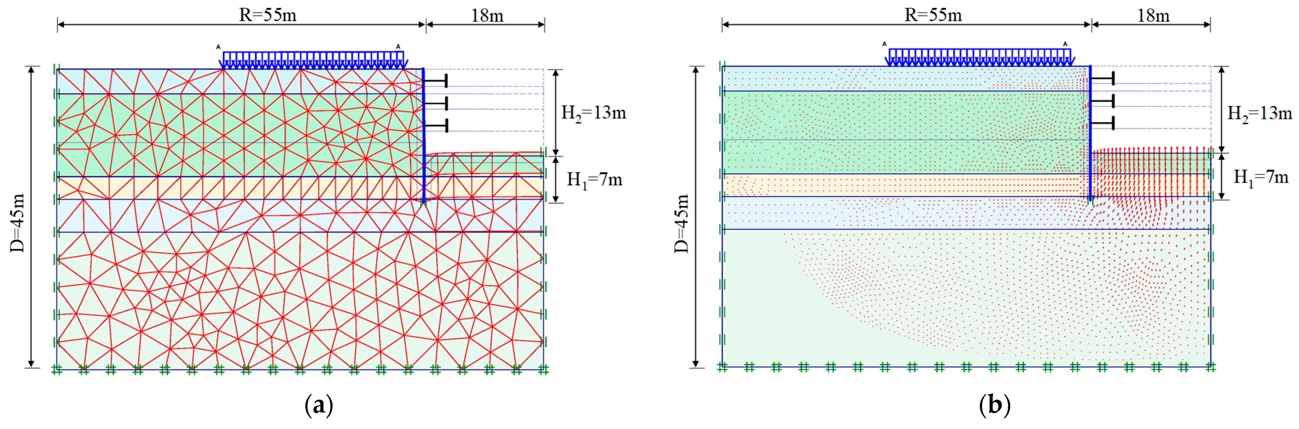
- Internal bracing system: The excavation follows a top-down sequence with staged excavation and horizontal bracing. The bracing system consists of three levels, using H-beams as support structures. The excavation profile is shown in Figure A1b.
- (3)
- Excavation steps: The first stage involves excavation to GL.−2.6 m and the installation of the first-level bracing. The second stage involves excavation to GL.−6.0 m and the installation of the second-level bracing. The third stage involves excavation to GL.−9.3 m and the installation of the third-level bracing. The fourth stage involves excavation to the final excavation bottom at GL.−13.0 m. Due to the lower groundwater level in the research case area, the excavation depth mainly consists of the gravel layer, resulting in lower lateral pressures on the retaining wall compared to typical cases.
3.2.3. Assumptions for Analysis
- The excavation process is assumed to exhibit plane strain behavior.
- Referring to the analysis model proposed by Fan, the influence range of the backside of the retaining wall is considered [47]. For the analysis, the range (B) extends at least four times the excavation depth beyond the retaining wall. The vertical range (D) is determined by adding twice the penetration depth (3H1 + H2) to the length of the continuous wall, assuming a uniform distributed load of 1.5 t/m2 acting on the ground surface.
- Based on the site conditions, considering the excavation depth, plan shape, support system configuration, and soil layer boundaries, an analysis mesh is established. The boundary elements of the mesh are assumed to have no horizontal or lateral displacements outside the influence range.
- The stiffness of the retaining wall is reduced by 70% based on general empirical values.
- The continuous wall and support elements are simulated using beam elements.
- An analysis is performed using 15-node triangular elements.
- At the bottom of the wall, if there is penetration into rock or gravel layers beyond a certain depth (more than 1.5 m), based on the reference monitoring data from relevant cases, no significant horizontal displacements are observed; therefore, in the analysis, horizontal displacements are constrained at the bottom of the wall.
3.2.4. Determination of Strata and Structural Parameters
3.2.5. Analysis Procedure
- Case Study 1
- (1)
- First-stage excavation to GL.−2.7 m;
- (2)
- Installation of ST1 at GL.−1.9 m;
- (3)
- Second-stage excavation to GL.−4.7 m;
- (4)
- Installation of ST2 at GL.−3.9 m;
- (5)
- Third-stage excavation to GL.−7.1 m;
- (6)
- Installation of ST3 at GL.−6.3 m;
- (7)
- Fourth-stage excavation to GL.−10.4 m;
- (8)
- Installation of ST4 at GL.−9.6 m;
- (9)
- Fifth-stage excavation to GL.−13.7 m;
- (10)
- Installation of ST5 at GL.−12.9 m;
- (11)
- Sixth-stage excavation to the final excavation bottom at GL.−17.3 m (analysis mode ends at this point).
- Case Study 2
- (1)
- First-stage excavation to GL.−2.6 m;
- (2)
- Installation of ST1 at GL.−1.8 m;
- (3)
- Second-stage excavation to GL.−6.0 m;
- (4)
- Installation of ST2 at GL.−5.2 m;
- (5)
- Third-stage excavation to GL.−9.3 m;
- (6)
- Installation of ST3 at GL.−8.5 m;
- (7)
- Fourth-stage excavation to the final excavation bottom at GL.−13.0 m (analysis and simulation end at this point).
3.2.6. Feedback Analysis
3.2.7. Results and Discussion of the Case Studies
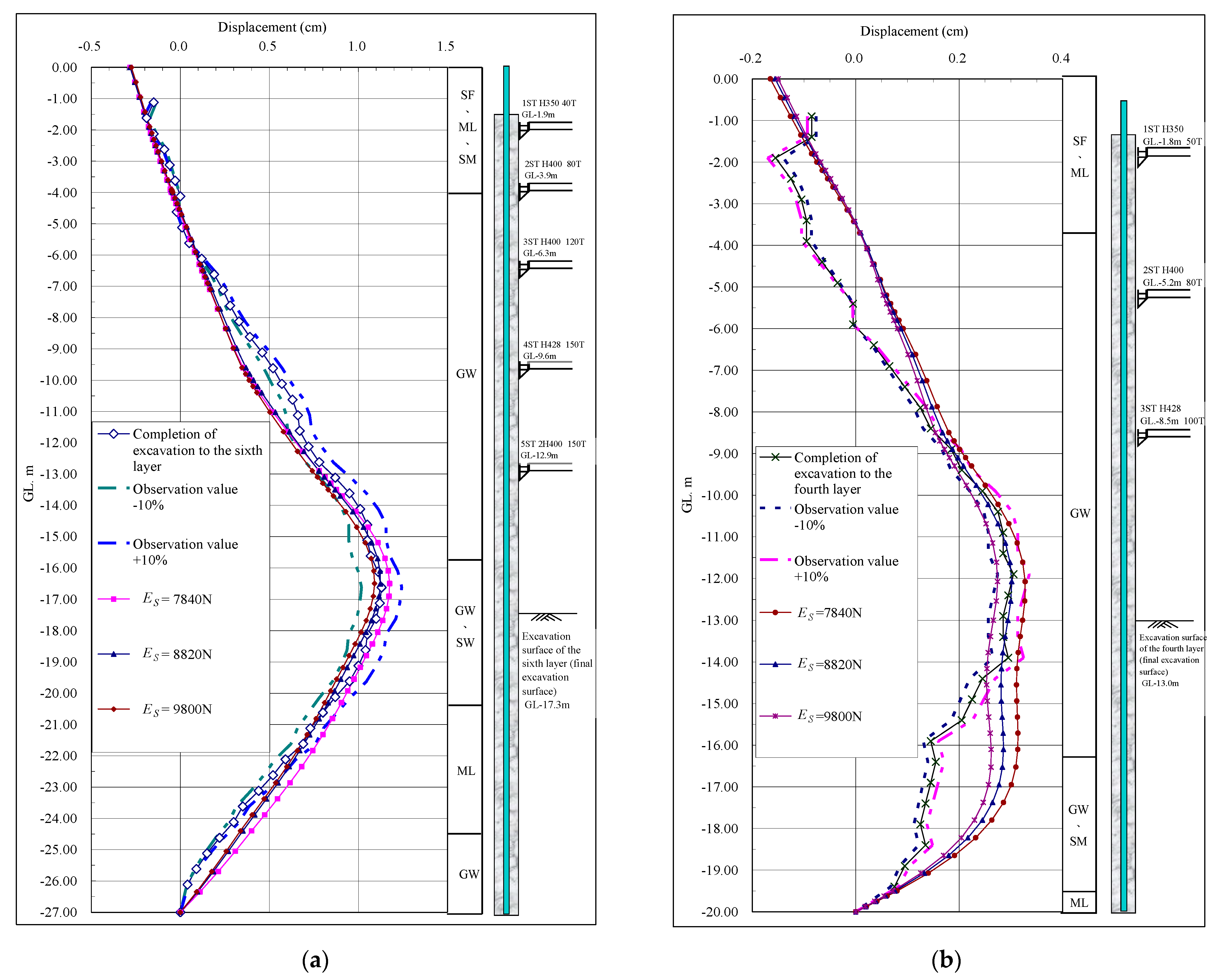
- Referring to the case studies in this research and numerous monitoring data, it was observed that when the bottom of the wall penetrates into a rock layer or gravel layer at a certain depth (greater than 1.5 m), there is no horizontal displacement at the bottom of the wall; therefore, in the analysis, the horizontal displacement at the bottom of the wall is restrained. The analysis results show consistency with the actual monitoring data in terms of the maximum deformation location and the trend of the wall displacement curve, indicating that this basic assumption of the analysis is reasonable.
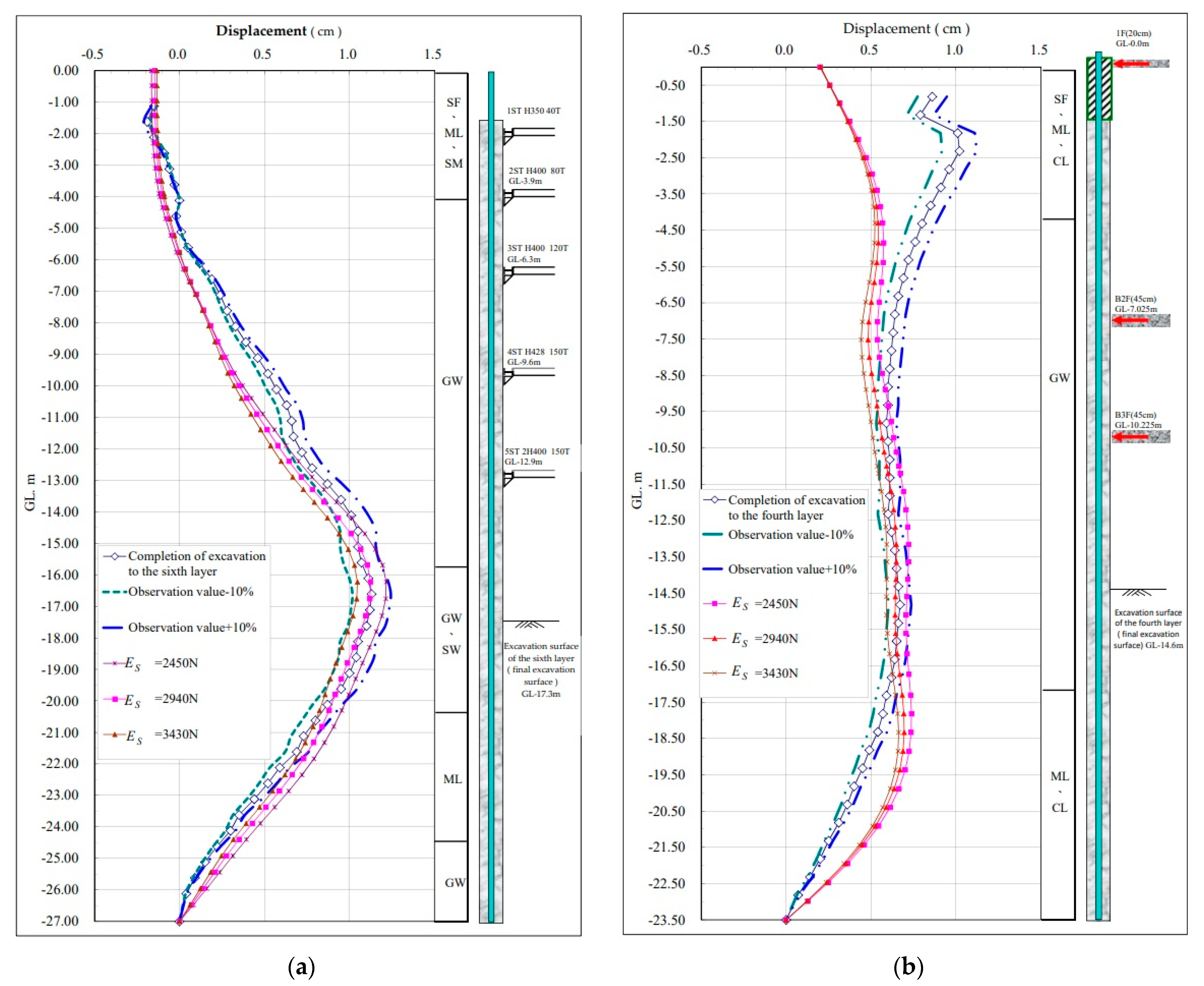
- The feedback results from both case studies indicate that assuming an N-value of 100 for the second layer of the gravel layer, within the range of the soil elastic modulus between 7840 kN/m2 and 9800 kN/m2, it is possible to reasonably estimate the maximum deformation and its occurrence location during the final excavation stage, with a tolerance of ±10% based on the actual monitoring data.
3.3. Discussion of the Findings
- Based on the feedback analysis results from actual cases, it is shown that when using a reasonable soil elastic modulus for predictive analysis, more accurate final excavation deformation quantities can be obtained. In the Xindian area, this range is between 7840 kN/m2; and 9800 kN/m2;. These results align with the empirical formulas derived from the prior research of Kuo et al. and Hou et al. on the gravel layer in Baguashan. The elastic modulus in Baguashan was found to range from 88,200 kN/m2; to 833,000 kN/m2; [48,49].
- In this study, a parameter feedback analysis was conducted based on actual cases in the Xindian area of Taiwan, suggesting that this research method can be applied to regions with similar geological conditions. Extending this approach to various regions can yield a broader range of research results, which could be valuable as references in engineering design.
4. SoilWorks Numerical Simulation
4.1. Analysis Methods and Models
4.2. Sensitivity Analysis
4.2.1. Analysis Description
4.2.2. Assumed Cases
- Basic Case Description for Sandy Soil Layer
- (1)
- Analysis Assumptions
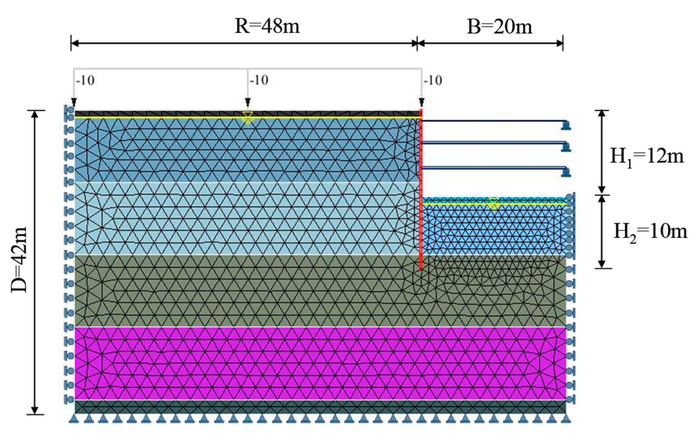
- The length and width of the excavation area are both 40 m, with a depth of excavation of 12 m (H1) and a depth of wall penetration of 10 m (H2). The total length of the continuous wall is 22 m.
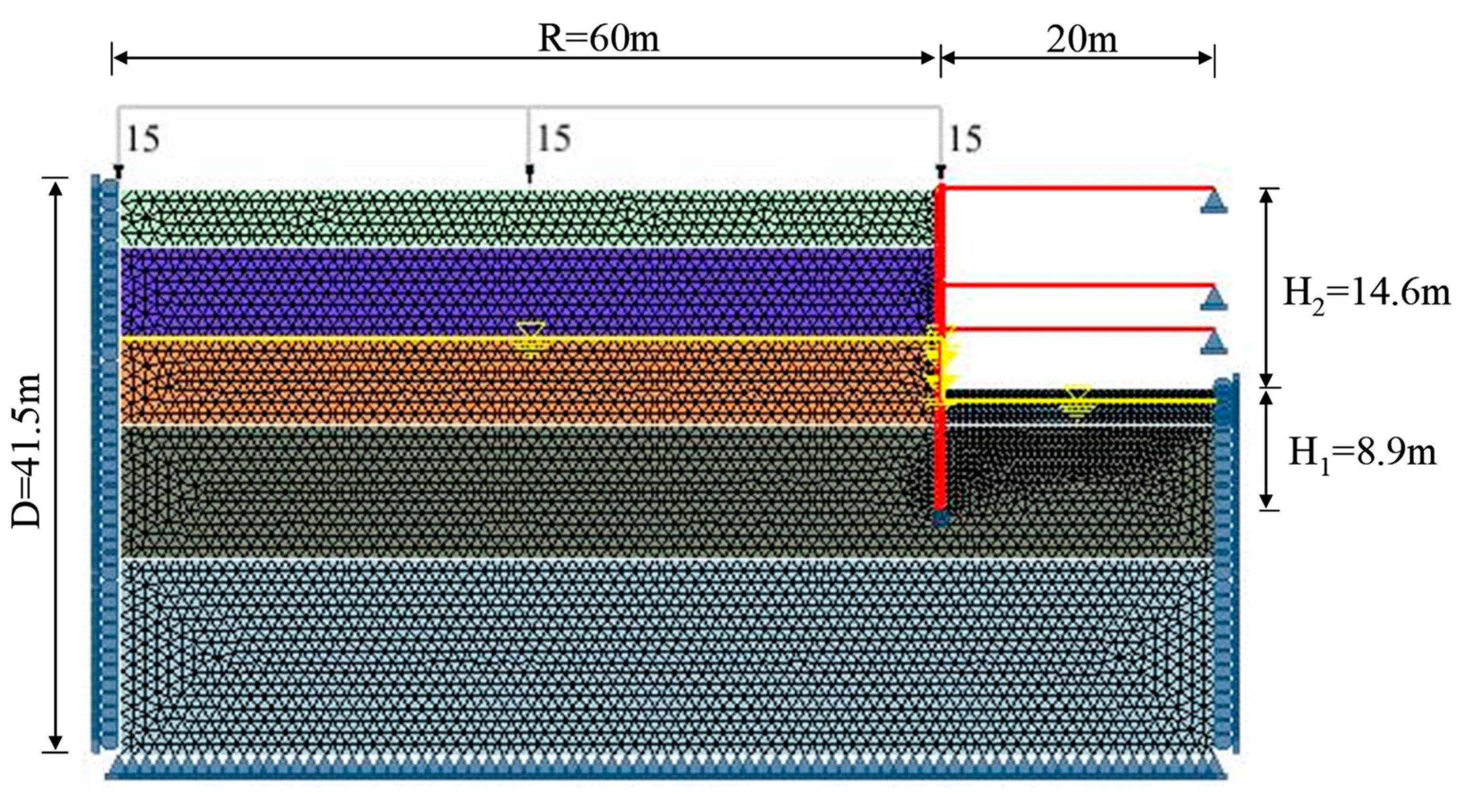
- The analysis model adopts a symmetric single-side mode, with a horizontal analysis length (B) of half the original excavation length, which is 20 m. Considering the influence range of the backside of the retaining wall, a distance of at least four times the excavation depth (R = 12 × 4 = 48 m) is considered. The vertical range (D) is taken as the length of the continuous wall (H1 + H2) plus twice the penetration depth (H2), assuming a uniformly distributed load of 10 kN/m2 acting on the ground surface. The detailed model diagram for the simulated case analysis is shown in Figure 6.
- Considering the excavation depth, support system configuration, and soil layer boundaries, a complete analysis mesh is established. The boundary elements of the mesh are assumed to have no horizontal or lateral displacements outside the influence range.
- The retaining wall is simulated using beam elements, with the stiffness reduced by 70% based on general empirical values. The input parameters used in the analysis are detailed in Table A3.
- The support system is simulated using truss elements, with the stiffness reduced by 50% based on general empirical values. The input parameters used in the analysis are detailed in Table A4.
- The analysis is conducted using 15-node triangular elements.
- (2)
- Geology and Groundwater
- Basic Case Description for Clay Soil Layer
- (1)
- Analysis Assumptions
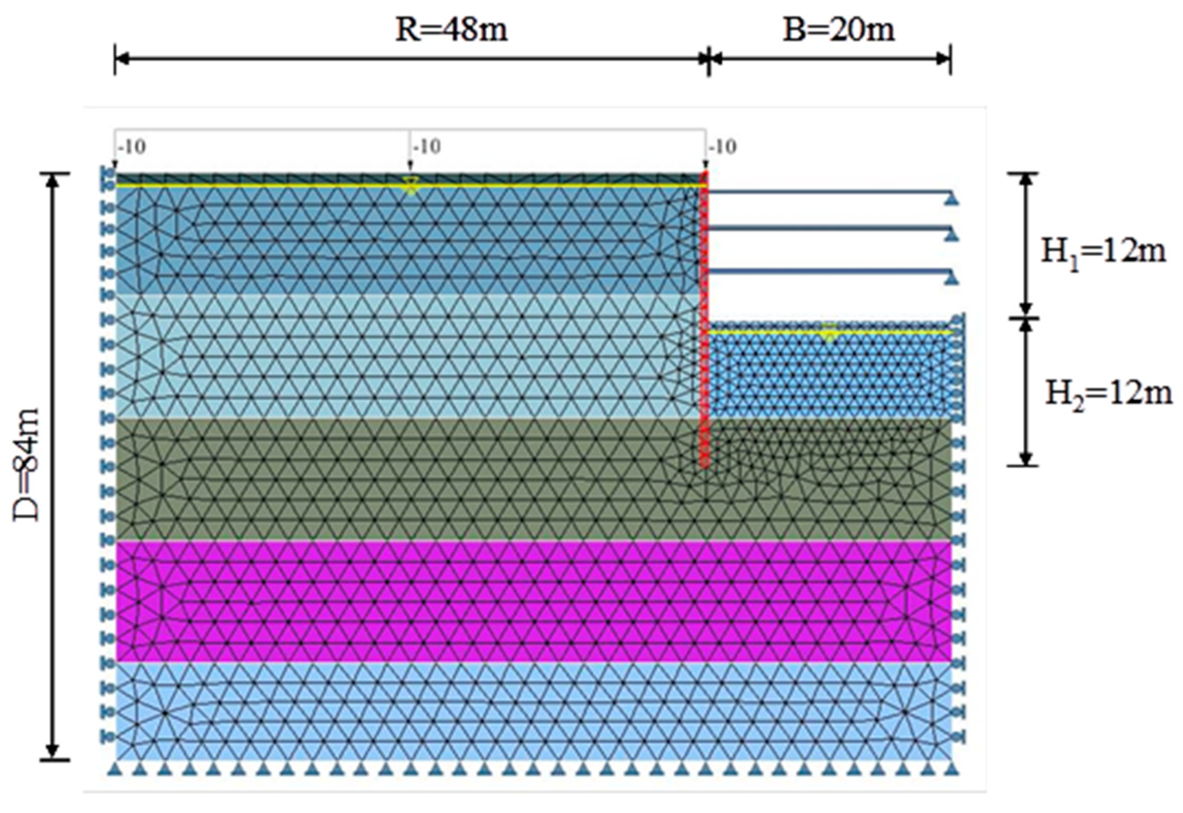
- The length and width of the excavation area are both 40 m, with a depth of excavation of 12 m (H1) and a depth of wall penetration of 12 m (H2). The total length of the continuous wall is 24 m.
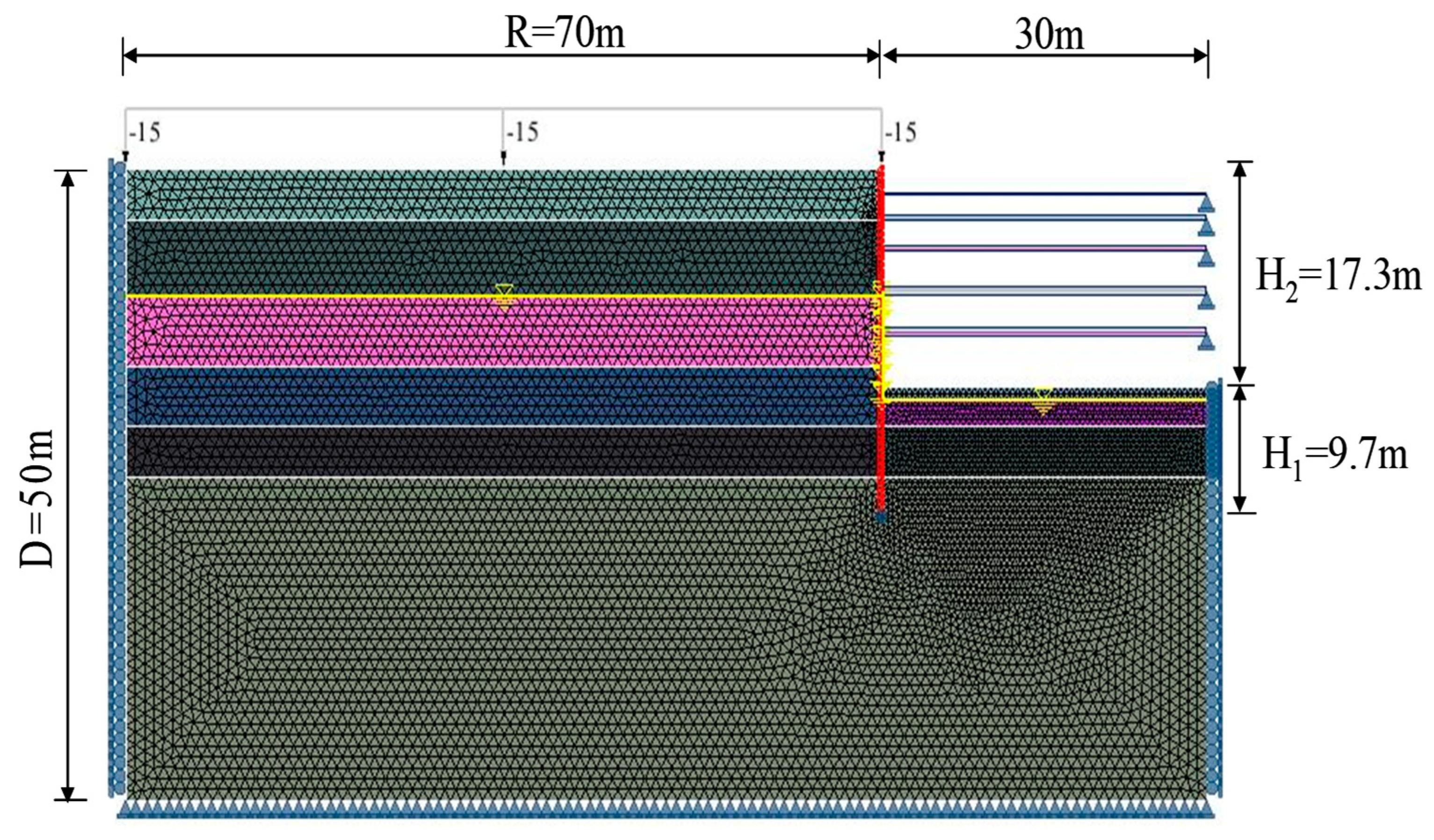
- The analysis model adopts a symmetric single-side mode, with a horizontal analysis length (B) of half the original excavation length, which is 20 m. Considering the influence range of the backside of the retaining wall, a distance of at least four times the excavation depth (R = 12 × 4 = 48 m) is considered. The vertical range (D) is taken as the length of the continuous wall (H1 + H2) plus twice the penetration depth (H2), assuming a uniformly distributed load of 10 kN/m2 acting on the ground surface. The detailed model diagram for the simulated case analysis is shown in Figure 7.
- Considering the excavation depth, support system configuration, and soil layer boundaries, a complete analysis mesh is established. The boundary elements of the mesh are assumed to have no horizontal or lateral displacements outside the influence range.
- The retaining wall is simulated using beam elements, and the input parameters used in the analysis are detailed in Table A3.
- The support system is simulated using truss elements, and the input parameters used in the analysis are detailed in Table A4.
- An analysis is conducted using 15-node triangular elements.
- (2)
- Geology and Groundwater
4.2.3. Parameter Range
- Friction Angle (Φ)
- Soil Elastic Modulus (Es)
4.2.4. Analysis Results
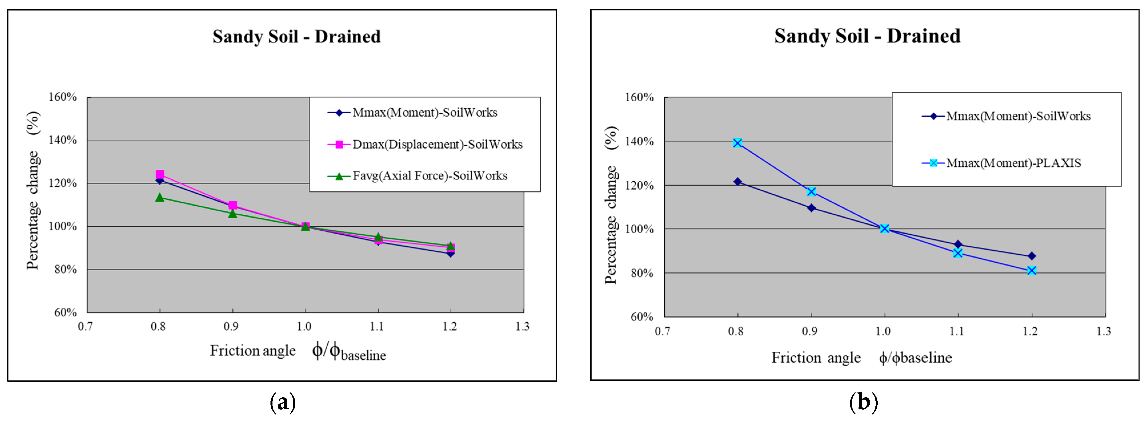
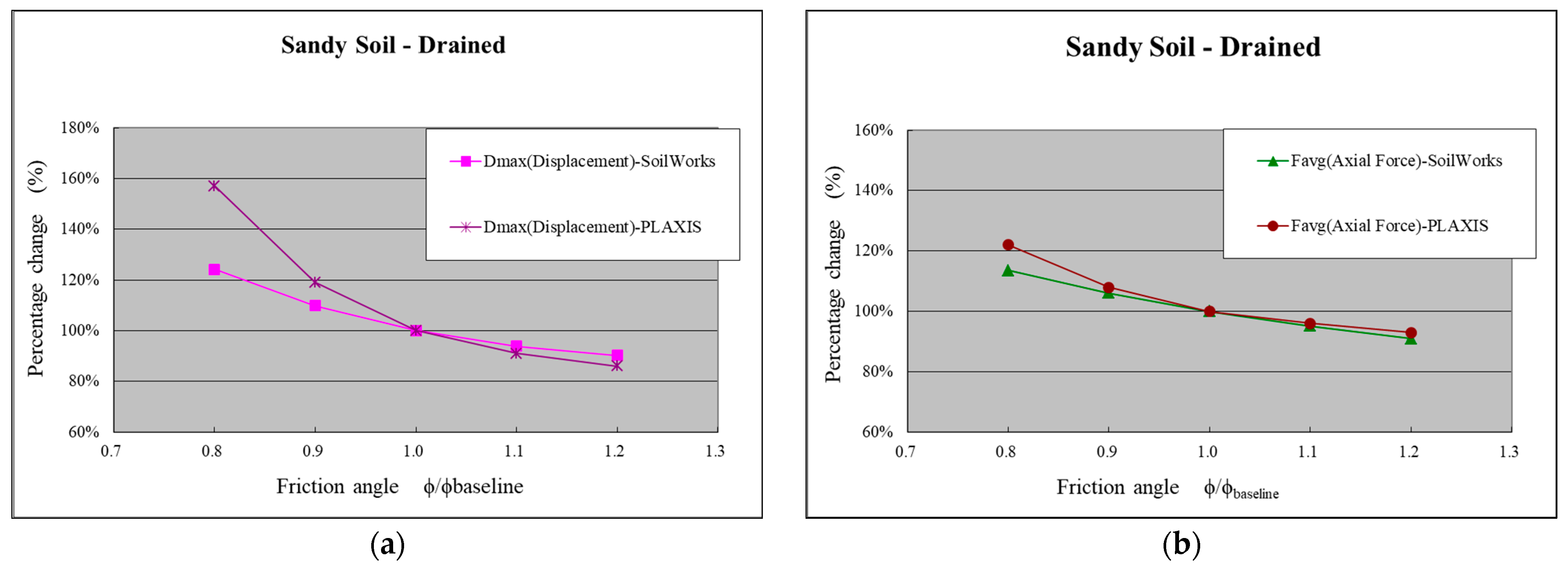
- Sensitivity Analysis of Friction Angle
- (1)
- Sandy Soil Layer
- (2)
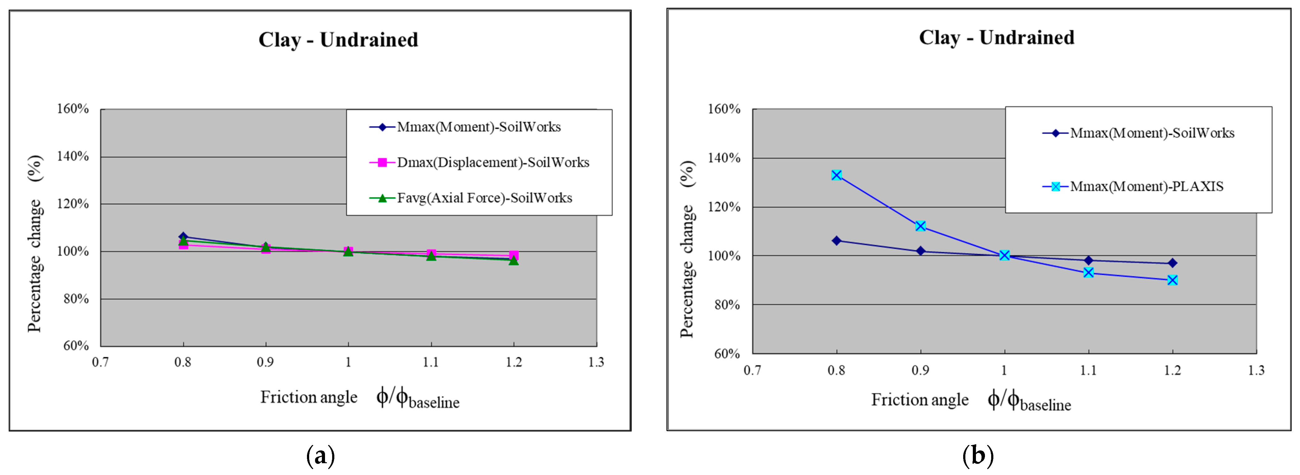
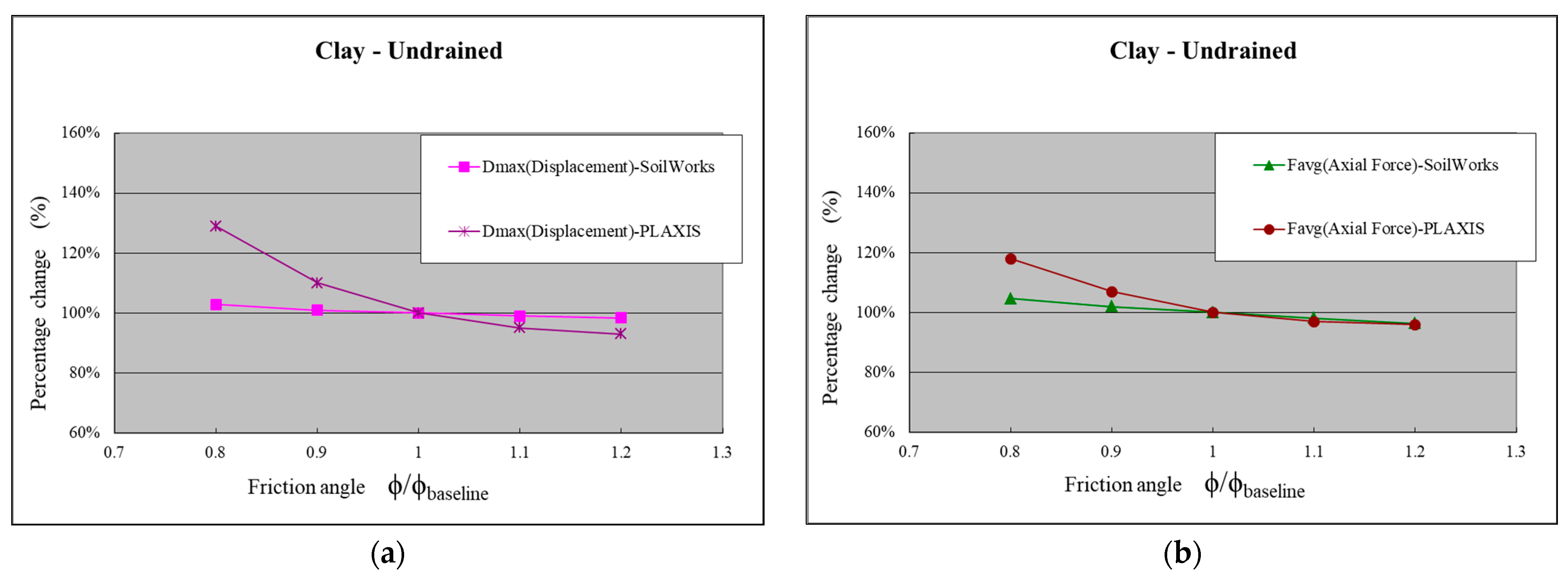
- Clay Layer (Undrained Condition)
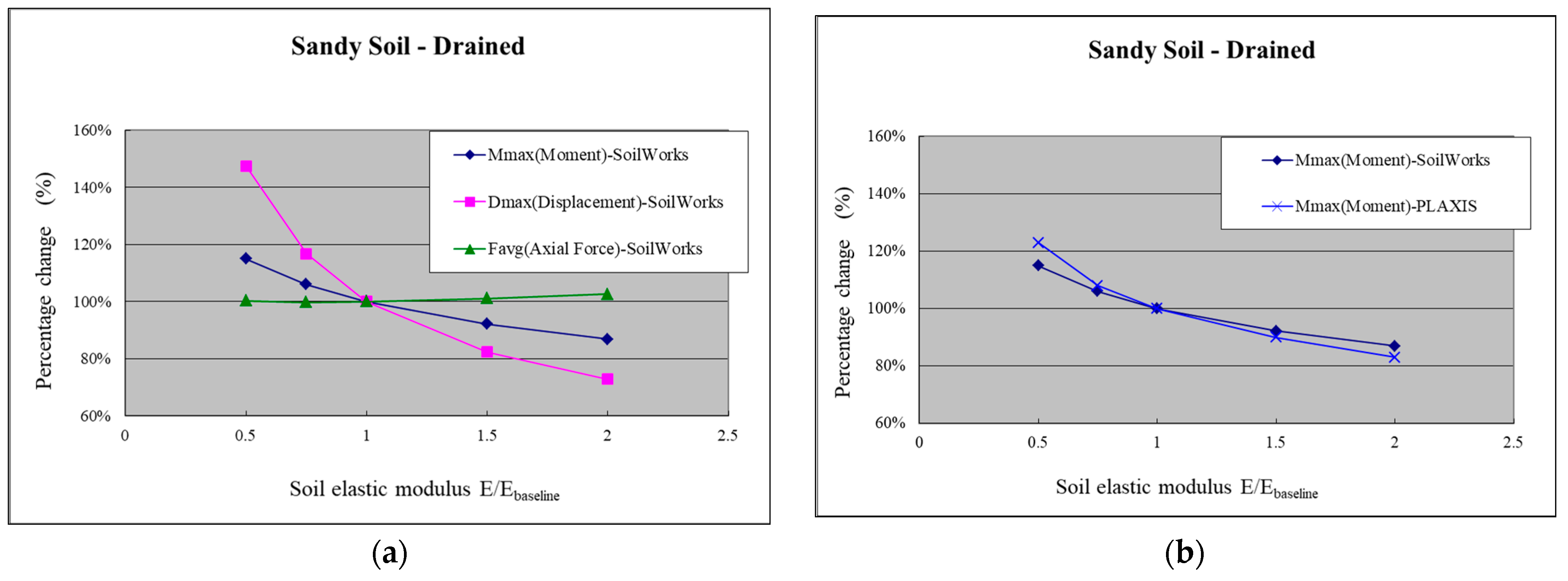
- Sensitivity Analysis of Soil Elastic Modulus
- (1)
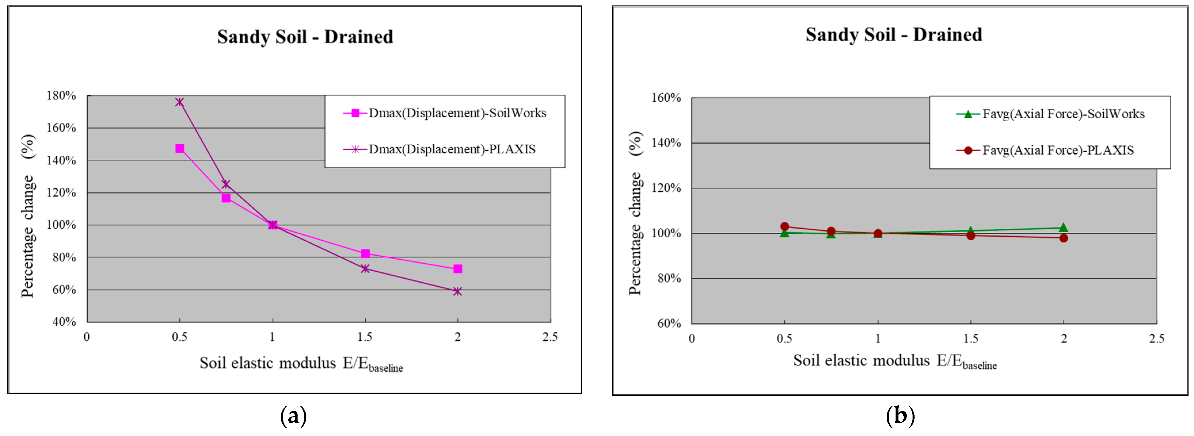
- Sandy Soil
- (2)
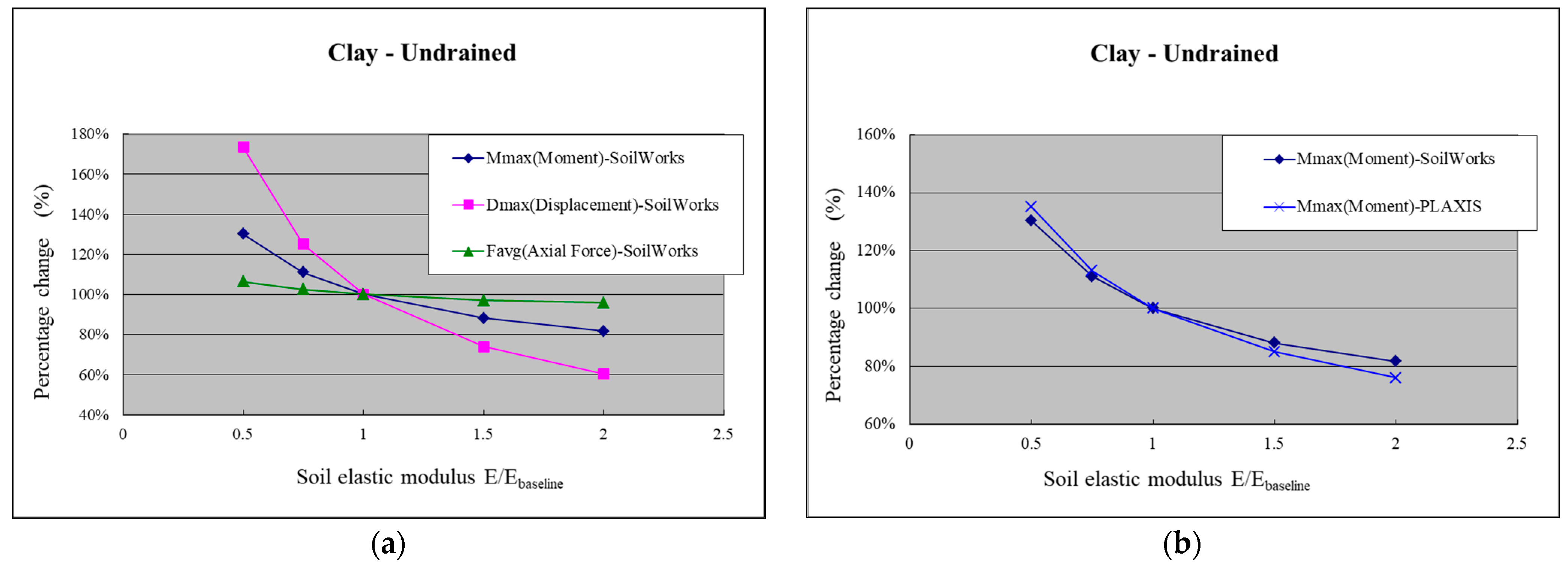
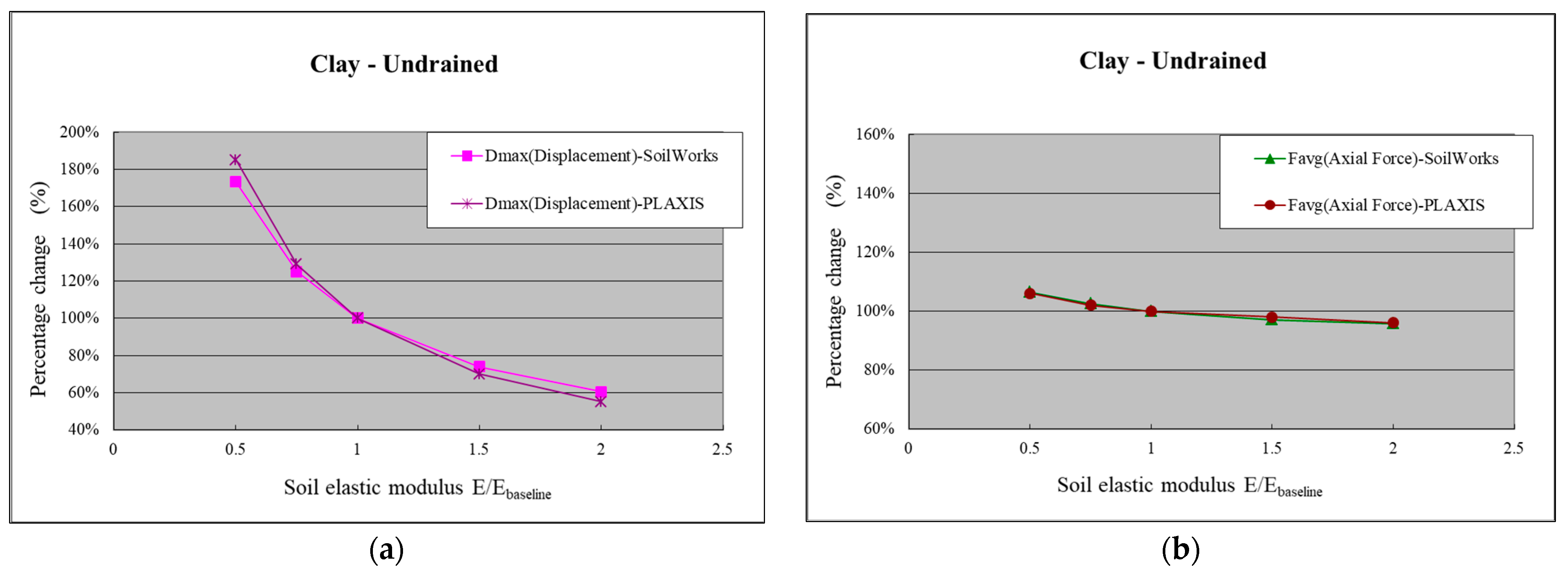
- Clay Layer (Undrained Condition)
- (3)
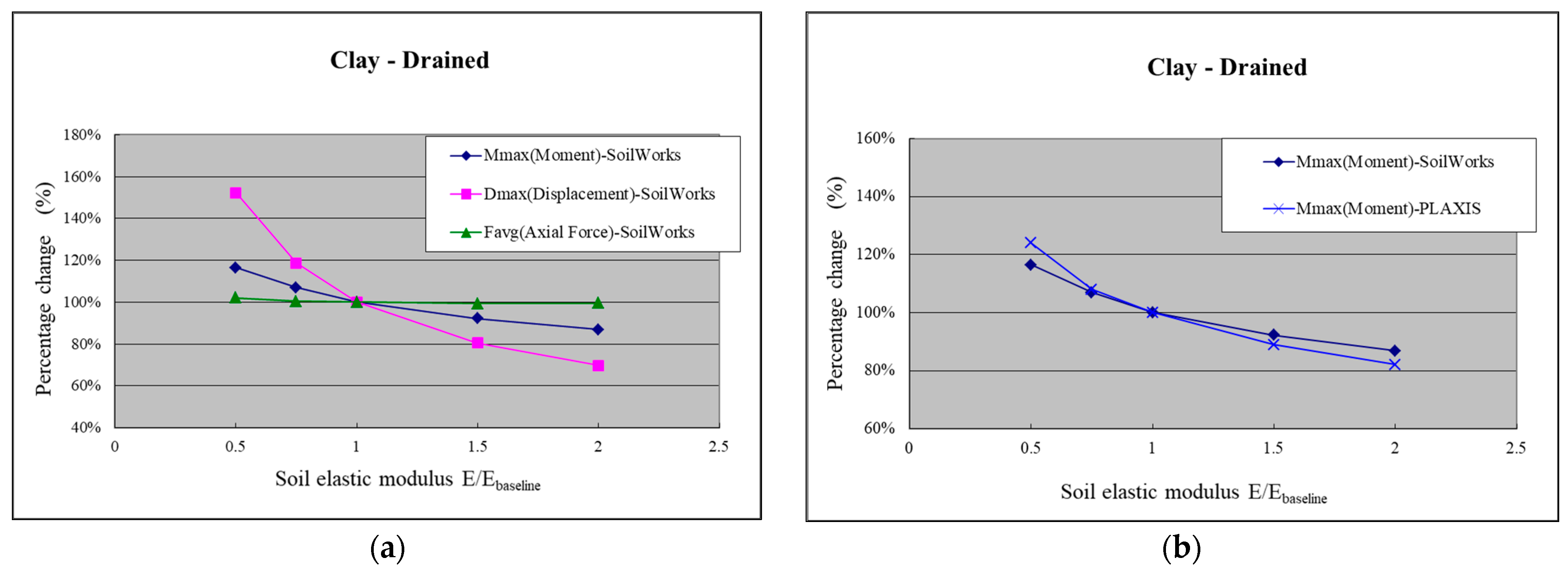
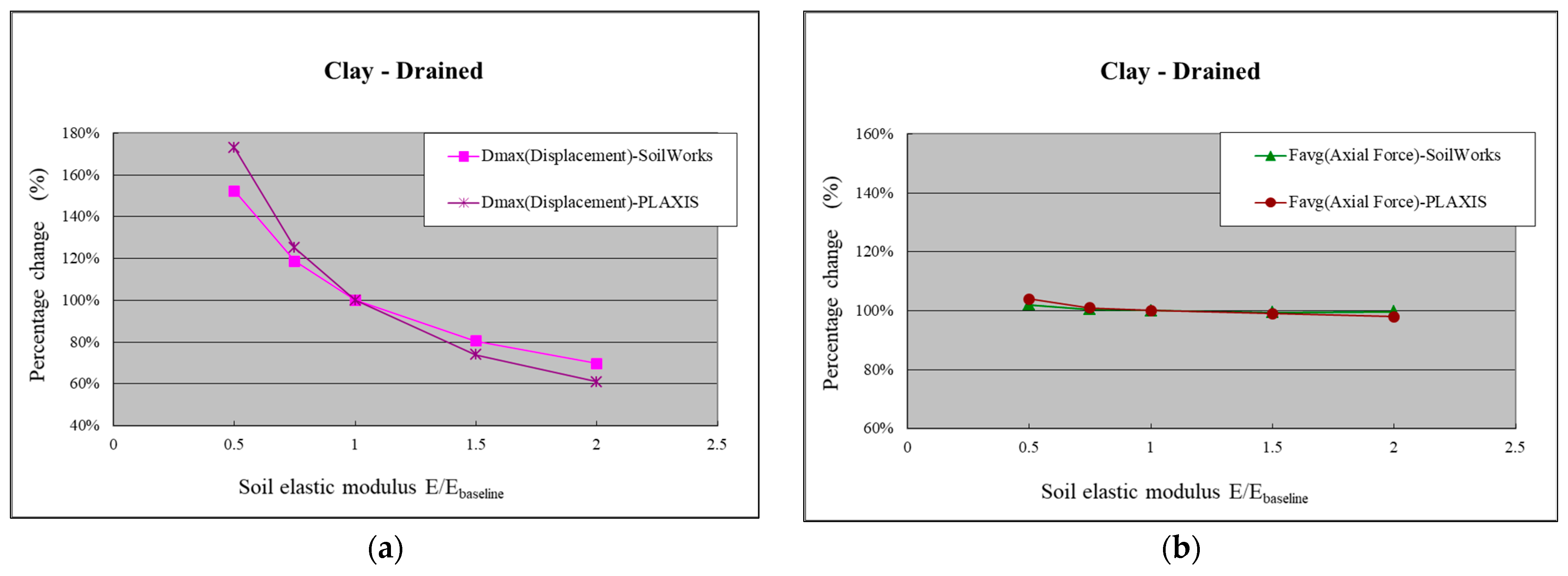
- Clay Layer (Drained Condition)
4.3. Case Study
4.3.1. Description and Input Parameter Selection for Case 3
- Site Description
- Subsurface Strata
- (1)
- Fill layer: Consists of yellow-brown sandy clay, silty clay, and silty clay with mud. The thickness is approximately 4.3 m, and the N-values range from 1 to 19.
- (2)
- Gravel layer: Contains egg-sized gravel interbedded with yellow-brown silty clay. The thickness is approximately 11 m, and the N-values range from 15 to above 50.
- (3)
- Gray sandy clay layer: Consists of gray sandy clay, silty clay, and sandy clay. The thickness is 9.6 m, and the N-values range from 7 to 50 (increasing to 50 when encountering gravel).Gravel layer: Contains egg-sized gravel interbedded with yellow-brown silty sand. The thickness is greater than 8.8 m, and the N-values are all above 50.
- Foundation Excavation Plan
- (1)
- Geotechnical facilities: The excavation depth is 14.6 m, and the foundation type is a raft foundation. The retaining structure consists of 80 cm thick continuous walls, with a depth of 23.5 m.
- (2)
- Support system: The inverted construction method is adopted for the site, which involves staged excavation and construction of underground floor slabs. The support structures used during the excavation process are 1F, B2FL, and B3FL.
- (3)
- Excavation steps: The excavation is carried out in four stages. In the first stage, the excavation is lowered to GL.−2.5 m to construct the 1F floor slab. In the second stage, the excavation is lowered to GL.−8.0 m to construct the B2F floor slab (GL.−7.025 m). In the third stage, the excavation is lowered to GL.−11.2 m to construct the B3F floor slab (GL.−10.225 m). Finally, in the fourth stage, the excavation is lowered to the final excavation bottom at GL.−14.6 m.
- Determination of Soil and Structural Parameters
- Basic Assumptions
- (1)
- The excavation process is assumed to exhibit plane strain behavior.
- (2)
- Considering the influence range behind the retaining wall, the analysis range (B) extends at least four times the excavation depth beyond the retaining wall. The vertical range (D) is obtained by adding twice the penetration depth (3H1 + H2) to the length of the retaining wall. A uniform distributed load of 15 kN/m2 is assumed to act on the ground surface.
- (3)
- Based on the site conditions, including the excavation depth, shape, support system configuration, and soil layer boundaries, a mesh is created for the analysis. The boundary elements of the mesh are assumed to have no horizontal or lateral displacements outside the influence range.
- (4)
- The stiffness of the retaining wall is reduced by 70% based on empirical experience, while the stiffness of the floor slab is reduced by 25%.
- (5)
- The retaining walls and floor slabs are simulated using beam elements.
- (6)
- The analysis is conducted using 15-node triangular elements.
- (7)
- Based on the observation of previous cases, when the bottom of the retaining wall penetrates the gravel layer to a certain depth (more than 1.5 m below the bottom), no significant horizontal displacements are observed; therefore, in the analysis, horizontal displacements at the bottom of the retaining wall are restricted.
- Analysis Procedure
- (1)
- Perform the first-stage excavation to GL.−2.5 m;
- (2)
- Construct the 1FL at GL.−0.0 m;
- (3)
- Perform the second-stage excavation to GL.−8.0 m;
- (4)
- Construct the B2FL at GL.−7.025 m;
- (5)
- Perform the third-stage excavation to GL.−11.2 m;
- (6)
- Construct the B3FL at GL.−10.225 m;
- (7)
- Perform the fourth-stage excavation to GL.−14.6 m (reaching the bottom of the excavation, analysis simulation ends at this point).
4.3.2. Feedback Analysis
4.4. Discussion of Results
- A sensitivity analysis of the effective friction angle in SoilWorks was conducted. The results indicate that Mmax and Dmax are more sensitive to a smaller friction angle in the sandy and clayey (drained) layers; however, in the clayey (undrained) layer, the sensitivity to the friction angle is lower. Furthermore, comparing the sensitivity analysis results with PLAXIS, it was found that SoilWorks generally exhibits lower sensitivity.
- A sensitivity analysis of the soil elastic modulus in SoilWorks was conducted. The results show that in both the sandy and clayey (drained and undrained) layers, the elastic modulus values of the soil have a greater influence on Mmax and Dmax. Comparing the sensitivity analysis results with PLAXIS, it was found that SoilWorks exhibits lower sensitivity than PLAXIS for Dmax, while the sensitivities of Mmax and Favg are comparable between the two.
- From the sensitivity analysis, it can be concluded that the friction angle and soil elastic modulus are two parameters that have a relatively high sensitivity to the displacement of the retaining wall.
- Consistent with the previous PLAXIS analysis, when the bottom of the wall reaches a certain depth into rock or gravel layers (more than 1.5 m), there is no horizontal displacement observed at the bottom of the wall; therefore, in the analysis, horizontal displacement at the bottom of the wall was restrained. The analysis results demonstrate consistency with the actual monitoring data in terms of the maximum deformation location and the trend of the wall displacement curve, indicating that this basic assumption in the analysis is reasonable.
- A feedback analysis was conducted using Case 1, followed by validation using Case 3. The results indicate that under the assumption of N = 100 for the second layer of gravel, within the soil elastic modulus range 2450N~3430N (kN/m2), a reasonable estimation of the maximum deformation and its occurrence location during the final excavation stage can be achieved under the conditions of gravel layers in the Xindian area.
5. Conclusions
5.1. Conclusions
- Sensitivity Analysis of Effective Friction Angle in SoilWorksThe results indicate that the maximum bending moment and maximum displacement are more sensitive to smaller friction angles in both sandy and clayey (drained) soil layers. In contrast, the sensitivity to the friction angle is lower in the undrained clay layers. Furthermore, upon comparing the sensitivity analysis results with PLAXIS, it was observed that SoilWorks generally exhibits lower sensitivity.
- Sensitivity Analysis of Soil Elastic Modulus in SoilWorksThe results show that the maximum bending moment and maximum displacement are more sensitive to changes in soil elastic modulus values, regardless of whether these relate to the sand layer or the clay layer. Comparing the sensitivity analysis results with PLAXIS, it was observed that SoilWorks has lower sensitivity to the maximum displacement but similar sensitivity to the maximum bending moment and average axial force.
- A parameter feedback analysis was conducted for deep excavation using two-dimensional PLAXIS and SoilWorks analysis programs. Based on the feedback analysis results from various practical cases, it was found that for the gravel layer in Xindian area, soil elastic modulus values of 7840 N/m2; to 9800 N/m2; in PLAXIS and 2450 N/m2; to 3430 N/m2; in SoilWorks can reasonably estimate the maximum deformation in the final excavation stage.
5.2. Recommendations
- Based on the sensitivity analysis of the effective friction angle and soil elastic modulus in PLAXIS and SoilWorks, as well as the analysis of three different excavation depths and construction methods, it is evident that the soil elastic modulus has a significant impact on wall displacement. This impact becomes more pronounced with larger excavation scales; therefore, careful evaluation of the input parameters should be exercised during the analysis.
- A parameter feedback analysis was conducted in PLAXIS and SoilWorks exclusively for cases involving gravel layers in the Xindian area. The findings may not be directly applicable to other regions with similar geological conditions. Since gravel layer characteristics can vary across different regions, it is advisable to follow the research process outlined in this study when analyzing specific areas. This approach can provide a broader range of research results for reference to designers and engineers in the future.
Author Contributions
Funding
Institutional Review Board Statement
Informed Consent Statement
Data Availability Statement
Conflicts of Interest
Appendix A

| Strata Description | N | γt | Total Stress Effective Stress | Total Stress Effective Stress | ||
|---|---|---|---|---|---|---|
| Φ | Φ′ | |||||
| The Average Thickness of Each Layer | Value | kN/m3 | kN/m2 | ˚ | kN/m2 | ˚ |
| 1.5~19 (5) | 19.3 | * 9.8 | * 21 | 0 | 30 |
| Average thickness 4.0 m | ||||||
| 15~>50 (40) | 21.6 | - | - | * 4.9 | * 38 |
| Average thickness 11.7 m | ||||||
| 20~58 (35) | 21.1 | - | - | * 0 | * 38 |
| Average thickness 4.6 m | ||||||
| 12~26 (16) | 19.4 | 9.8 | 24 | 0 | 32 |
| Average thickness 0.5 m | ||||||
| >50 (100) | * 22.1 | - | - | * 9.8 | * 40 |
| Average thickness 10.0 m (hole bottom) | ||||||
| Strata Description | N | γt | Total Stress Effective Stress | Total stress Effective Stress | ||
|---|---|---|---|---|---|---|
| Φ | Φ’ | |||||
| The Average Thickness of Each Layer | Value | kN/m3 | kN/m2 | ˚ | kN/m2 | ˚ |
| 5~17 (7) | 19.4 | 9.8 | 22 | * 0 | * 30 |
| Average thickness 3.7 m | ||||||
| 22~>50 (40) | 21.9 | - | - | * 4.9 | * 38 |
| Average thickness 12.4 m | ||||||
| 16~31 (23) | 21.1 | - | - | * 0 | * 34 |
| Average thickness 3.4 m | ||||||
| 11~20 (13) | 19.5 | 9.8 | 24 | 0 | 31 |
| Average thickness 4.9 m | ||||||
| >50 (100) | * 22.1 | - | - | * 9.8 | * 40 |
| Average thickness 11.1 m (hole bottom) | ||||||
| Thickness(m) | E (kN/m2) | I (m4/m) | Reduction Factor | 0.7EA (kN/m) | 0.7EI (kNm2/m) |
|---|---|---|---|---|---|
| 0.6 | 2.17 × 10⁷ | 0.018 | 0.7 | 9.13 × 10⁶ | 2.739 × 10⁵ |
| Number of Supporting Layers | Supporting Position | Model | A (cm2) | 0.5EA (kN) | Preload (kN/m) |
|---|---|---|---|---|---|
| 1ST | GL.−1.5 m | 1 × H 350 | 173.9 | 1.826 × 10⁶ | 125 |
| 2ST | GL.−4.5 m | 2 × H 350 | 347.7 | 3.651 × 10⁶ | 200 |
| 3ST | GL.−8.0 m | 2 × H 400 | 437.4 | 4.592 × 10⁶ | 300 |
| Depth (m) | Soil Classification | (kN/m2) | Φ’(o) | γunsat(kN/m3) | γsat(kN/m3) | Es (kN/m2) | υ |
|---|---|---|---|---|---|---|---|
| 10 | SM | 1 | 30 | 20 | 21 | 12,500 | 0.32 |
| 20 | SM | 1 | 30 | 20 | 21 | 37,500 | 0.32 |
| 30 | SM | 1 | 30 | 20 | 21 | 62,500 | 0.32 |
| 40 | SM | 1 | 30 | 20 | 21 | 87,500 | 0.32 |
| 42 | SM | 1 | 30 | 20 | 21 | 812,500 | 0.32 |
| Depth (m) | Soil Classification | (kN/m2) | Φ’(o) | γunsat(kN/m3) | γsat(kN/m3) | Es(kN/m2) | υ |
|---|---|---|---|---|---|---|---|
| 10 | CL | 5 | 20 | 19 | 18 | 10,000 | 0.35 |
| 20 | CL | 5 | 23 | 19 | 18 | 18,750 | 0.35 |
| 30 | CL | 5 | 25 | 19 | 18 | 31,250 | 0.35 |
| 40 | CL | 5 | 28 | 19 | 18 | 43,750 | 0.35 |
| 42 | CL | 5 | 30 | 19 | 18 | 56,250 | 0.35 |
| SM | Mmax | Percentage Change | Dmax | Percentage Change | Favg | Percentage Change |
|---|---|---|---|---|---|---|
| (kN-m) | (%) | (mm) | (%) | (kN/m) | (%) | |
| 0.5E | 371.32 | 115% | 48.483 | 147% | 246.1 | 100% |
| 0.75E | 342.43 | 106% | 38.368 | 117% | 244.9 | 100% |
| 1.0E | 323.07 | 100% | 32.872 | 100% | 245.4 | 100% |
| 1.5E | 297.63 | 92% | 27.075 | 82% | 248.2 | 101% |
| 2.0E | 280.69 | 87% | 23.941 | 73% | 251.7 | 103% |
| SM | Mmax Percentage Change | Dmax Percentage Change | Favg Percentage Change | |||
|---|---|---|---|---|---|---|
| Siolworks | PLAXIS | Siolworks | PLAXIS | Siolworks | PLAXIS | |
| 0.5E | 115% | 123% | 147% | 176% | 100% | 103% |
| 0.75E | 106% | 108% | 117% | 125% | 100% | 101% |
| 1.0E | 100% | 100% | 100% | 100% | 100% | 100% |
| 1.5E | 92% | 90% | 82% | 73% | 101% | 99% |
| 2.0E | 87% | 83% | 73% | 59% | 103% | 98% |
| CL (Undrained) | Mmax | Percentage Change | Dmax | Percentage Change | Favg | Percentage Change |
|---|---|---|---|---|---|---|
| (kN-m) | (%) | (mm) | (%) | (kN/m) | (%) | |
| 0.5E | 327.72 | 130% | 81.231 | 173% | 257.0 | 106% |
| 0.75E | 279.50 | 111% | 58.627 | 125% | 247.5 | 103% |
| 1.0E | 251.72 | 100% | 46.867 | 100% | 241.4 | 100% |
| 1.5E | 221.83 | 88% | 34.688 | 74% | 234.4 | 97% |
| 2.0E | 205.65 | 82% | 28.341 | 60% | 231.2 | 96% |
| CL (Undrained) | Mmax Percentage Change | Dmax Percentage Change | Favg Percentage Change | |||
|---|---|---|---|---|---|---|
| Siolworks | PLAXIS | Siolworks | PLAXIS | Siolworks | PLAXIS | |
| 0.5E | 130% | 135% | 173% | 185% | 106% | 106% |
| 0.75E | 111% | 113% | 125% | 129% | 103% | 102% |
| 1.0E | 100% | 100% | 100% | 100% | 100% | 100% |
| 1.5E | 88% | 85% | 74% | 70% | 97% | 98% |
| 2.0E | 82% | 76% | 60% | 55% | 96% | 96% |
| CL (Drained) | Mmax | Percentage Change | Dmax | Percentage Change | Favg | Percentage Change |
|---|---|---|---|---|---|---|
| (kN-m) | (%) | (mm) | (%) | (kN/m) | (%) | |
| 0.5E | 439.21 | 116% | 71.259 | 152% | 260.5 | 102% |
| 0.75E | 403.60 | 107% | 55.556 | 119% | 256.3 | 100% |
| 1.0E | 377.30 | 100% | 46.818 | 100% | 255.4 | 100% |
| 1.5E | 348.20 | 92% | 37.725 | 81% | 253.6 | 99% |
| 2.0E | 327.66 | 87% | 32.639 | 70% | 254.3 | 100% |
| CL (Drained) | Mmax Percentage Change | Dmax Percentage Change | Favg Percentage Change | |||
|---|---|---|---|---|---|---|
| Siolworks | PLAXIS | Siolworks | PLAXIS | Siolworks | PLAXIS | |
| 0.5E | 116% | 124% | 152% | 173% | 102% | 104% |
| 0.75E | 107% | 108% | 119% | 125% | 100% | 101% |
| 1.0E | 100% | 100% | 100% | 100% | 100% | 100% |
| 1.5E | 92% | 89% | 81% | 74% | 99% | 99% |
| 2.0E | 87% | 82% | 70% | 61% | 100% | 98% |
| Strata Description | N | Total Stress Effective Stress | Total Stress Effective Stress | |||
|---|---|---|---|---|---|---|
| Φ | Φ’ | |||||
| Bottom Depth of Each Layer | Value | kN/m3 | kN/m2 | ˚ | kN/m2 | ˚ |
| 1~19 | 20.1 | 9.8 | 24 | 0 | 28 |
| Average thicknes 4.3 m | ||||||
| 15~>50 | 22.1 | - | - | * 4.9 | * 38 |
| Average thicknes 13.0 m | ||||||
| 7~50 | 20.0 | 4.9 | 26 | 0 | 31 |
| Average thicknes 9.8 m | ||||||
| >50 | * 22.1 | - | - | * 9.8 | * 40 |
| Average thicknes 11.1 m (hole bottom) | ||||||
Appendix B

References
- Hong, R.J. Comprehensive Investigation and Study of Underground Geology and Engineering Environment in Taipei Basin: Research on Stratigraphic Distribution; Central Geological Survey Report; Report No. 83-009; Central Geological Survey, MOEA: New Taipei, Taiwan, 1994.
- Liu, Z.L. Seismic Microzonation Map of Taipei Basin. Master’s Thesis, National Central University, Taoyuan, Taiwan, 1994. [Google Scholar]
- Li, X.H. Engineering Geological Zoning of Taipei City. Geotech. Technol. 1996, 25–34. [Google Scholar] [CrossRef]
- PLAXIS BV. Plaxis Version 8 Manual; Delft University of Technology & PLAXIS b.v.: Amsterdam, The Netherlands, 2006. [Google Scholar]
- Huang, C.Y. Application of Neural Networks in Predicting Deformation of Deep Excavation Walls. Master’s Thesis, National Taiwan Ocean University, Keelung, Taiwan, 2002. [Google Scholar]
- Chen, J.Q.; Ji, S.Y. Study on Characteristics and Deep Excavation Behavior of Soft Soil Layers (I): Research on Analysis Program for Interaction between Deep Excavation Soil and Support; Chunghsing Engineering Consulting Corporation: Taipei, Taiwan, 1996. [Google Scholar]
- Ji, S.Y.; Chen, J.Q. Numerical Simulation of Time-Dependent Deep Excavation Construction. In Proceedings of the 7th Geotechnical Engineering Conference, Hsinchu, Taiwan, 11–15 June 1997; pp. 609–615. [Google Scholar]
- Tang, Y.G. Study on Soil Parameter Identification for Deep Excavation Analysis. Ph.D. Dissertation, National Taiwan University of Science and Technology, Taipei, Taiwan, 1998. [Google Scholar]
- Xie, B.G.; Ou, Z.Y. Deep Excavation Analysis under Undrained Conditions Using a Pseudo-Plastic Model. J. China Civ. Eng. 2000, 12, 703–713. [Google Scholar]
- He, Z.D. Deep Excavation Analysis in Soft Soil Layers. Master’s Thesis, National Taipei University of Technology, Taipei, Taiwan, 2004. [Google Scholar]
- Chen, C.G. Preliminary Study on Simulating the Behavior of Excavation and Support using RIDO and PLAXIS Programs. Master’s Thesis, National Ilan University, Yilan, Taiwan, 2011. [Google Scholar]
- Wang, K.; Li, W.; Sun, H.; Pan, X.; Diao, H.; Hu, B. Lateral Deformation Characteristics and Control Methods of Foundation Pits Subjected to Asymmetric Loads. Symmetry 2021, 13, 476. [Google Scholar] [CrossRef]
- Yazici, M.F.; Keskin, S.N. Optimum Design of Multi-anchored Larssen Type Sheet Pile Wall for Temporary Construction Works. Geomech. Eng. 2021, 27, 1–11. [Google Scholar] [CrossRef]
- Hong, L.; Chen, L.; Wang, X. Reliability Analysis of Serviceability Limit State for Braced Excavation Considering Multiple Failure Modes in Spatially Variable Soil. Buildings 2022, 12, 722. [Google Scholar] [CrossRef]
- Nguyen, B.P.; Ngo, C.P.; Tran, T.D.; Bui, X.C.; Doan, N.-P. Finite Element Analysis of Deformation Behavior of Deep Excavation Retained by Diagram Wall in Ho Chi Minh City. Indian Geotech. J. 2022, 52, 989–999. [Google Scholar] [CrossRef]
- Rahmani, F.; Hosseini, S.M.; Khezri, A.; Maleki, M. Effect of grid-form deep soil mixing on the liquefaction-induced foundation settlement, using numerical approach. Arab. J. Geosci. 2022, 15, 1112. [Google Scholar] [CrossRef]
- Maleki, M.; Imani, M. Active lateral pressure to rigid retaining walls in the presence of an adjacent rock mass. Arab. J. Geosci. 2022, 15, 152. [Google Scholar] [CrossRef]
- Maleki, M.; Mir Mohammad Hosseini, S. Seismic Performance of Deep Excavations Restrained by Anchorage System Using Quasi Static Approach. J. Seismol. Earthq. Eng. 2019, 21, 11–21. [Google Scholar] [CrossRef]
- Bjerrum, L. Observed versus Computed Settlement of Structures on Clay and Sand; Massachusetts Institute of Technology: Cambridge, MA, USA, 1964. [Google Scholar]
- D’Appolonia, D.J. Settlement of Spread Footing and Design. J. Soil Mech. Found. Div. 1970, 94, SM3. [Google Scholar]
- Shimons, N.E.; Menzies, B.K. A Short Course in Foundation Engineering; Butterworth & Co., Ltd.: London, UK, 1977. [Google Scholar]
- Bowles, J.E. Foundation Analysis and Design, 3rd ed.; Mc Graw-Hill: New York, NY, USA, 1982; pp. 1159–1177. [Google Scholar]
- Li, W.F.; Lai, Y.R.; Liao, N.H. Two-Dimensional Numerical Analysis Method for Soil Nailing Reinforced Slopes. Geotech. Technol. 2003, 98, 39–54. [Google Scholar]
- Hsieh, H.S.; Cheng, J.S.; Tsai, Z.H.; Yang, M.C. Practical Considerations for Continuous Wall Design Analysis. Geotech. Technol. 1996, 53, 35–44. [Google Scholar]
- Zhang, J.Z.; Chen, K.Q. Assessment of Sensitivity of Design Parameters on Deep Excavation and Retaining Wall. Geotech. Technol. 1999, 76, 17–24. [Google Scholar] [CrossRef]
- Qiu, Z.R. Study on Parameters of Deep Excavation in Sanchong-Luzhou Area. Master’s Thesis, National Taipei University of Technology, Taipei, Taiwan, 2007. [Google Scholar] [CrossRef]
- Hong, Z.S.; Zeng, L.L.; Cui, Y.J.; Cai, Y.Q.; Lin, C. Compression behaviour of natural and reconstituted clays. Géotechnique 2012, 62, 291–301. [Google Scholar] [CrossRef]
- Yao, Y.-P.; Hou, W.; Zhou, A.-N. UH model: Three-dimensional unified hardening model for over-consolidated clays. Géotechnique 2009, 59, 451–469. [Google Scholar] [CrossRef]
- Yao, Y.P.; Zhou, A.N. Non-isothermal unified hardening model: A thermo-elastoplastic model for clays. Géotechnique 2013, 63, 1328–1345. [Google Scholar] [CrossRef]
- Clough, G.W.; O’Rourke, T.D. Construction Induced Movements of In-Situ Walls. In Design and Performance of Earth Retaining Structures (GSP 25); ASCE: Reston, VA, USA, 1990; pp. 154–196. [Google Scholar]
- Jin, Y.F.; Yin, Z.Y.; Shen, S.L.; Hicher, P.Y. Selection of sand models and identification of parameters using an enhanced genetic algorithm. Int. J. Numer. Anal. Methods Geomech. 2016, 40, 1219–1240. [Google Scholar] [CrossRef]
- Cui, Q.-L.; Shen, S.-L.; Xu, Y.-S.; Wu, H.-N.; Yin, Z.-Y. Mitigation of Geohazards during Deep Excavations in Karst Regions with Caverns: A Case Study. Eng. Geol. 2015, 195, 16–27. [Google Scholar] [CrossRef]
- Elbaz, K.; Shen, S.L.; Cheng, W.C.; Arulrajah, A. Cutter-Disc Consumption during Earth Pressure Balance Tunnelling in Mixed Strata. Geotech. Eng. 2018, 171, 363–376. [Google Scholar] [CrossRef]
- Midas Co., Ltd. SoilWorks Program User Manual; Midas Co., Ltd.: New Taipei City, Taiwan, 2012. [Google Scholar]
- Hong, R.J. Preliminary Study on Composite Soil Engineering Properties. J. Eng. Natl. Taiwan Univ. 1978, 23, 1–12. [Google Scholar]
- Das, B. Fundamentals of Geotechnical Engineering, 3rd ed.; PWS: Boston, MA, USA, 1994; pp. 81–82. [Google Scholar]
- Ou, C.Y. Design Theory and Practice of Deep Excavation Method Analysis; Technology Press Co., Ltd.: Taipei City, Taiwan, 2002. [Google Scholar]
- Chuung, C.h. Investigation of the Influence of Mesh Boundaries on Finite Element Excavation Analysis Results. Master’s Thesis, National Taiwan University of Science and Technology, New Taipei, Taiwan, 2008. [Google Scholar]
- Maleki, M.; Khezri, A.; Nosrati, M.; Hosseini, S.M.M.M. Seismic amplification factor and dynamic response of soil-nailed walls. Model. Earth Syst. Environ. 2023, 9, 1181–1198. [Google Scholar] [CrossRef]
- Maleki, M.; Nabizadeh, A. Seismic performance of deep excavation restrained by guardian truss structures system using quasi-static approach. SN Appl. Sci. 2021, 3, 417. [Google Scholar] [CrossRef]
- Maleki, M.; Mir Mohammad Hosseini, S.M. Assessment of the Pseudo-static seismic behavior in the soil nail walls using numerical analysis. Innov. Infrastruct. Solut. 2022, 7, 262. [Google Scholar] [CrossRef]
- Kenkul Engineering Co., Ltd. Completion Report of Foundation Construction Safety Observation for Jianglinchun Phase 1 Building Project 2005a; Kenkul Engineering Co., Ltd.: New Taipei City, Taiwan, 2005. [Google Scholar]
- Lin, C.M. Numerical Simulation of Excavation in Gravel Layers. Master’s Thesis, National Taiwan Ocean University, Keelung, Taiwan, 2011. [Google Scholar]
- Chunglian Engineering Consultants Co., Ltd. Geological Investigation and Analysis Report for Land Parcels 34 and 110, Dafeng Section, Xindian City, Taipei County; Chunglian Engineering Consultants Co., Ltd.: New Taipei City, Taiwan, 2003. [Google Scholar]
- Kenkul Engineering Co., Ltd. Completion Report of Foundation Construction Safety Observation for Jianglinchun Phase 2 Building Project; Kenkul Engineering Co., Ltd.: New Taipei City, Taiwan, 2006. [Google Scholar]
- Kenkul Engineering Co., Ltd. Geological Investigation and Analysis Report for Land Parcels 62-1 and Seven Others, Dafeng Section, Xindian City, Taipei County, 2005b; Kenkul Engineering Co., Ltd.: New Taipei City, Taiwan, 2005. [Google Scholar]
- Fan, C.Y. Finite Element Analysis of Mutual Effects of Adjacent Excavation Sites. Master’s Thesis, Feng Chia University, Taichung, Taiwan, 2005. [Google Scholar]
- Guo, T.Y. Numerical Analysis Study of Deformation Behavior in Gravel Layer Tunnels. Master’s Thesis, National Cheng Kung University, Tainan, Taiwan, 1999. [Google Scholar]
- Hou, Z.A. Feedback Analysis of Excavation Procedure and Optimal Support Types in Cobble Gravel Layers. Master’s Thesis, National Chung Hsing University, Taichung, Taiwan, 2001. [Google Scholar]
- Chunglian Engineering Consultants Co., Ltd. Geological Investigation and Analysis Report for Land Lots with Nine Parcel Numbers, Section 21, 22, 22–1, 24, 24-1, 26, 26–1, 69, and 79, Xindian District, Taipei County, 2006; Chunglian Engineering Consultants Co., Ltd.: New Taipei City, Taiwan, 2006. [Google Scholar]


| Depth (m) | Soil Classification | Use N Value | (kN/m2) | Φ’ (o) | γunsat (kN/m3) | γsat (kN/m3) | Es (kN/m2) | υ |
|---|---|---|---|---|---|---|---|---|
| 0.0~4.0 | SF, ML, SM | 5 | 0 | 30 | 19.3 | 19.5 | 15,000 N | 0.33 |
| 4.0~15.7 | GW | 40 | 4.9 | 38 | 21.6 | 22.0 | 7840 N–9800 N | 0.28 |
| 15.7~20.3 | GW, SW | 35 | 0 | 38 | 21.1 | 21.4 | 7840 N–9800 N | 0.28 |
| 20.3~24.4 | ML | 16 | 0 | 32 | 19.4 | 19.7 | 100,000 N | 0.32 |
| 24.4~33.0 | GW | 100 | 9.8 | 40 | 22.1 | 22.3 | 7840 N–9800 N | 0.26 |
| Depth (m) | Soil Classification | Use N Value | (kN/m2) | Φ’ (o) | γunsat (kN/m3) | γsat (kN/m3) | Es (kN/m2) | υ |
|---|---|---|---|---|---|---|---|---|
| 0.0~3.7 | SF, ML | 7 | 0 | 30 | 19.4 | 19.5 | 24,000 N | 0.33 |
| 3.7~16.1 | GW | 40 | 4.9 | 38 | 21.9 | 22.0 | 7840 N–9800 N | 0.28 |
| 16.1~19.5 | GM, SM | 23 | 0 | 34 | 21.1 | 21.4 | 7840 N–9800 N | 0.31 |
| 19.5~24.4 | ML | 13 | 0 | 31 | 19.5 | 19.7 | 100,000 N | 0.33 |
| 24.4~35.5 | GP, GM | 100 | 9.8 | 40 | 22.1 | 22.3 | 7840 N–9800 N | 0.26 |
| Thickness (m) | E (kN/m2) | I (m4/m) | Reduction Factor | 0.7EA (kN/m) | 0.7EI (kNm2/m) |
|---|---|---|---|---|---|
| 0.7 | 2.35 × 10⁷ | 0.028583 | 0.7 | 1.13 × 10⁷ | 4.60 × 10⁵ |
| Number of Supporting Layers | Supporting Position | Model | A (cm2) | 0.7EA (kN) | Preload (kN/m) |
|---|---|---|---|---|---|
| 1ST | GL.−1.9 m | 1 × H 350 | 173.9 | 2.51 × 10⁶ | 65 |
| 2ST | GL.−3.9 m | 1 × H 400 | 218.7 | 3.15 × 10⁶ | 131 |
| 3ST | GL.−6.3 m | 1 × H 400 | 218.7 | 3.15 × 10⁶ | 196 |
| 4ST | GL.−9.6 m | 2 × H 400 | 437.4 | 6.30 × 10⁶ | 245 |
| 5ST | GL.−12.9 m | 2 × H 400 | 437.4 | 6.30 × 10⁶ | 245 |
| Thickness (m) | E (kN/m2) | I (m4/m) | Reduction Factor | 0.7EA (kN/m) | 0.7EI (kNm2/m) |
|---|---|---|---|---|---|
| 0.6 | 2.35 × 10⁷ | 0.018 | 0.7 | 9.66 × 10⁶ | 2.90 × 10⁵ |
| Number of Supporting Layers | Supporting Position | Model | A (cm2) | 0.7EA (kN) | Preload (kN/m) |
|---|---|---|---|---|---|
| 1ST | GL.−1.8 m | 1 × H 350 | 173.9 | 2.51 × 10⁶ | 82 |
| 2ST | GL.−3.9 m | 1 × H 400 | 218.7 | 3.15 × 10⁶ | 131 |
| 3ST | GL.−8.5 m | 1 × H 428 | 360.65 | 5.20 × 10⁶ | 163 |
| SM | Mmax | Percentage Change | Dmax | Percentage Change | Favg | Percentage Change |
|---|---|---|---|---|---|---|
| (kN-m) | (%) | (mm) | (%) | (kN/m) | (%) | |
| 0.8Φ | 392.24 | 121% | 40.840 | 124% | 278.8 | 114% |
| 0.9Φ | 353.90 | 110% | 36.116 | 110% | 260.4 | 106% |
| 1.0Φ | 323.07 | 100% | 32.872 | 100% | 245.4 | 100% |
| 1.1Φ | 300.21 | 93% | 30.852 | 94% | 233.4 | 95% |
| 1.2Φ | 282.78 | 88% | 29.664 | 90% | 223.3 | 91% |
| SM | Mmax Percentage Change | Dmax Percentage Change | Favg Percentage Change | |||
|---|---|---|---|---|---|---|
| SoilWorks | PLAXIS | SoilWorks | PLAXIS | SoilWorks | PLAXIS | |
| 0.8Φ | 121% | 139% | 124% | 157% | 114% | 122% |
| 0.9Φ | 110% | 117% | 110% | 119% | 106% | 108% |
| 1.0Φ | 100% | 100% | 100% | 100% | 100% | 100% |
| 1.1Φ | 93% | 89% | 94% | 91% | 95% | 96% |
| 1.2Φ | 88% | 81% | 90% | 86% | 91% | 93% |
| CL (Undrained) | Mmax | Percentage Change | Dmax | Percentage Change | Favg | Percentage Change |
|---|---|---|---|---|---|---|
| (kN-m) | (%) | (mm) | (%) | (kN/m) | (%) | |
| 0.8Φ | 267.27 | 106% | 48.232 | 103% | 252.5 | 105% |
| 0.9Φ | 256.45 | 102% | 47.333 | 101% | 246.1 | 102% |
| 1.0Φ | 251.72 | 100% | 46.867 | 100% | 241.4 | 100% |
| 1.1Φ | 246.78 | 98% | 46.424 | 99% | 236.8 | 98% |
| 1.2Φ | 243.96 | 97% | 46.110 | 98% | 232.5 | 96% |
| CL (Undrained) | Mmax Percentage Change | Dmax Percentage Change | Favg Percentage Change | |||
|---|---|---|---|---|---|---|
| SoilWorks | PLAXIS | SoilWorks | PLAXIS | SoilWorks | PLAXIS | |
| 0.8Φ | 106% | 133% | 103% | 129% | 105% | 118% |
| 0.9Φ | 102% | 112% | 101% | 110% | 102% | 107% |
| 1.0Φ | 100% | 100% | 100% | 100% | 100% | 100% |
| 1.1Φ | 98% | 93% | 99% | 95% | 98% | 97% |
| 1.2Φ | 97% | 90% | 98% | 93% | 96% | 96% |
| Depth (m) | Soil Classification | Use N Value | (kN/m2) | Φ’ (o) | (kN/m3) | (kN/m3) | (kN/m2) | |
|---|---|---|---|---|---|---|---|---|
| 0.0~4.0 | SF, ML, SM | 5 | 0 | 30 | 19.3 | 19.5 | 12,250 N | 0.33 |
| 4.0~15.7 | GW | 40 | 4.9 | 38 | 21.8 | 22.0 | 2450 N–3430 N | 0.28 |
| 15.7~20.3 | GW, SW | 35 | 0 | 38 | 21.1 | 21.4 | 2450 N–3430 N | 0.28 |
| 20.3~24.4 | ML | 16 | 0 | 32 | 19.4 | 19.7 | 39,200 N | 0.32 |
| 24.4~33.0 | GW | 100 | 9.8 | 40 | 22.1 | 22.3 | 2450 N–3430 N | 0.26 |
| Depth (m) | Soil Classification | Use N Value | (kN/m2) | Φ’ (o) | (kN/m3) | (kN/m3) | (kN/m2) | |
|---|---|---|---|---|---|---|---|---|
| 0.0~4.0 | SF, ML, CL | 18 | 0 | 28 | 20.1 | 20.0 | 44,100 N | 0.347 |
| 4.0~15.7 | GW | 44 | 4.9 | 38 | 22.1 | 22.3 | 2450 N–3430 N | 0.263 |
| 15.7~20.3 | ML, SM | 18 | 0 | 31 | 20.0 | 19.3 | 44,100 N | 0.327 |
| 24.4~33.0 | GW | 100 | 9.8 | 40 | 22.1 | 22.3 | 2450 N–3430 N | 0.263 |
| Thickness (m) | E (kN/m2) | I (m4/m) | Reduction Factor | 0.7EA (kN/m) | 0.7EI (kNm2/m) |
|---|---|---|---|---|---|
| 0.8 | 2.13 × 10⁷ | 0.04267 | 0.7 | 1.19 × 10⁷ | 6.36 × 10⁵ |
| Number of Floors | Floor Position | Thickness (cm) | A (m2/m) | 0.25A (m2/m) | I (m4/m) | E (kN/m2) |
|---|---|---|---|---|---|---|
| 1F | GL.+0.0 m | 20 | 0.20 | 0.05 | 6.667 × 10⁻⁴ | 2.46 × 10⁷ |
| B2F | GL.−3.9 m | 45 | 0.45 | 0.1125 | 7.594 × 10⁻³ | 2.46 × 10⁷ |
| B3F | GL.−6.3 m | 45 | 0.45 | 0.1125 | 7.594 × 10⁻³ | 2.46 × 10⁷ |
Disclaimer/Publisher’s Note: The statements, opinions and data contained in all publications are solely those of the individual author(s) and contributor(s) and not of MDPI and/or the editor(s). MDPI and/or the editor(s) disclaim responsibility for any injury to people or property resulting from any ideas, methods, instructions or products referred to in the content. |
© 2023 by the authors. Licensee MDPI, Basel, Switzerland. This article is an open access article distributed under the terms and conditions of the Creative Commons Attribution (CC BY) license (https://creativecommons.org/licenses/by/4.0/).
Share and Cite
Wu, C.-Y.; Hsu, C.-F. Establishment of Localized Utilization Parameters for Numerical Simulation Analysis Applied to Deep Excavations. Appl. Sci. 2023, 13, 10127. https://doi.org/10.3390/app131810127
Wu C-Y, Hsu C-F. Establishment of Localized Utilization Parameters for Numerical Simulation Analysis Applied to Deep Excavations. Applied Sciences. 2023; 13(18):10127. https://doi.org/10.3390/app131810127
Chicago/Turabian StyleWu, Chien-Yi, and Chia-Feng Hsu. 2023. "Establishment of Localized Utilization Parameters for Numerical Simulation Analysis Applied to Deep Excavations" Applied Sciences 13, no. 18: 10127. https://doi.org/10.3390/app131810127