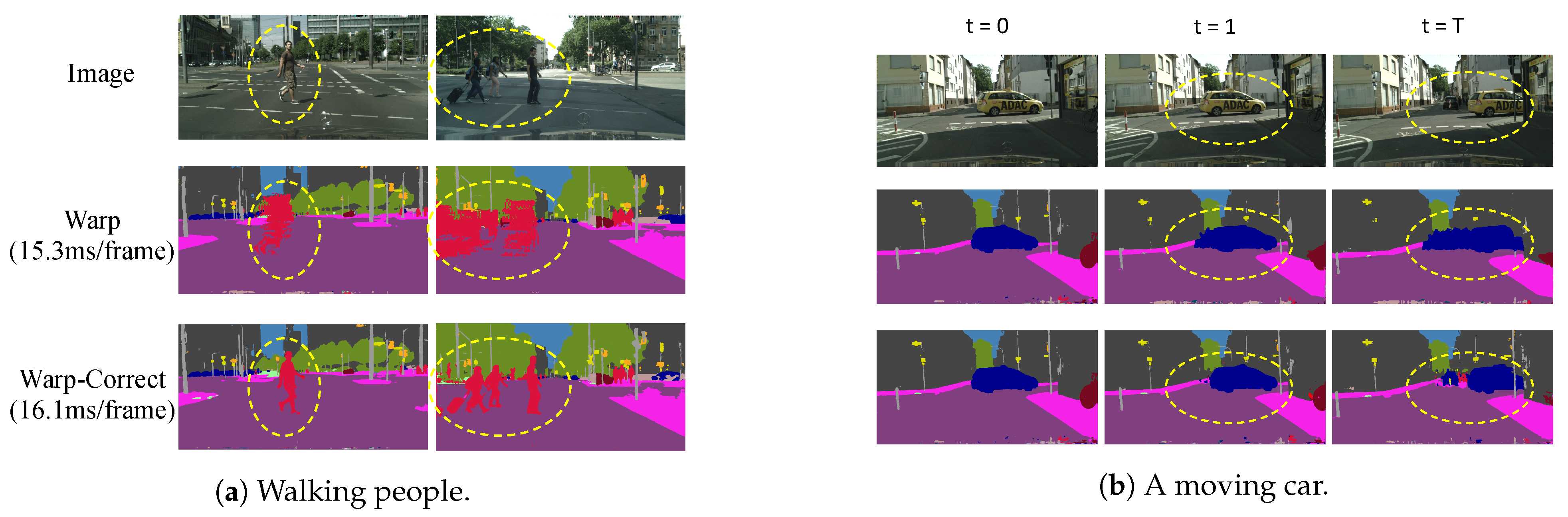
Article

Tamed Warping Network for High-Resolution Semantic Video Segmentation

College of Computer Science, Zhejiang University, Hangzhou 310027, China
*
Author to whom correspondence should be addressed.
These authors contributed equally to this work.
Appl. Sci. 2023, 13(18), 10102; https://doi.org/10.3390/app131810102
Submission received: 7 July 2023 / Revised: 3 September 2023 / Accepted: 4 September 2023 / Published: 7 September 2023
(This article belongs to the Special Issue Advances in Computer Vision and Semantic Segmentation)

Abstract

:
Recent approaches for fast semantic video segmentation have reduced redundancy by warping feature maps across adjacent frames, greatly speeding up the inference phase. However, the accuracy drops seriously owing to the errors incurred by warping. In this paper, we propose a novel framework and design a simple and effective correction stage after warping. Specifically, we build a non-key-frame CNN, fusing warped context features with current spatial details. Based on the feature fusion, our context feature rectification (CFR) module learns the model’s difference from a per-frame model to correct the warped features. Furthermore, our residual-guided attention (RGA) module utilizes the residual maps in the compressed domain to help CRF focus on error-prone regions. Results on Cityscapes show that the accuracy significantly increases from 67.3 % to 71.6 % , and the speed edges down from 65.5 FPS to 61.8 FPS at a resolution of 1024 × 2048 . For non-rigid categories, e.g., “human” and “object”, the improvements are even higher than 18 percentage points.

1. Introduction

Semantic video segmentation, an important task in the field of computer vision, aims to predict pixel-wise class labels for each frame in a video. It has been widely used for a variety of applications, e.g., autonomous driving [1], robot navigation [2], and video surveillance [3]. Since the seminal work of fully convolutional networks (FCNs) [4] was proposed, the accuracy of semantic segmentation has been significantly improved [5,6,7]. However, the computational cost and memory footprint of these high-quality methods are usually impractical to deploy in the aforementioned real-world applications, where only limited computational resources are available. Therefore, a fast solution to this dense prediction task is challenging and attracting more and more interest.
Prevailing fast methods for semantic video segmentation can be grouped into two major categories: per-frame and warping-based. Per-frame methods treat the video task as a stream of mutually independent image tasks and performs it frame by frame. This line of work takes several approaches to trade off accuracy for speed.
(1)
Reducing the resolution of the network input is a simple and widely used approach to boost the speed directly [8,9,10,11,12,13,14,15,16].
(2)
Adopting a lightweight network is standard practice on the systems with limited resources [9,10,17,18,19,20,21,22,23,24,25].
(3)
Designing an efficient network operator, e.g., dilated convolution, depth-wise separable convolution, and asymmetric convolution, is also explored in [26,27,28,29].
In general, per-frame methods adapt image models to video models with ease but do not utilize the inherent coherence of video frames.
In light of the visual continuity between adjacent video frames, warping-based methods [30,31,32,33,34] employ inter-frame motion estimation [31,33,34] to reduce temporal redundancy. Technically, this line of work treats a video clip as sequential groups of frames. Each group of frames consists of a key frame followed by multiple non-key frames. When the coming frame is a key frame, the warping-based model performs image segmentation as usual; otherwise, the model keeps the results of the preceding frame, warps the preceding results with the help of motion estimation, and uses the warped results as the results of the current frame. Since the warping operation is much faster than the inference of a CNN, the inference speed can be boosted significantly.
In spite of achieving fast speed, warping-based methods suffer a sharp drop in accuracy due to warping itself. As shown in Figure 1a, non-rigid moving objects such as walking people can change their shapes dramatically during walking. It is so difficult to estimate their motions that these objects become severely deformed after several non-key frames. Figure 1b shows a car occupying the central space at the beginning key frame (t = 0), but as the car moves to the right, another car, which was occluded at the key frame, appears at the later non-key frames. In this case, it is impossible to obtain the originally occluded car at later non-key frames by warping. Based on the above observations, the motion estimation that warping uses inevitably introduces errors, and errors accumulate along succeeding non-key frames, making the results almost unusable. Warping turns out to behave like a runaway fierce creature; the key to the issue is to tame it—to take advantage of its acceleration and to keep it under control.
To this end, we propose a novel “warp-and-correct” fast framework called the tamed warping network (TWNet) for high-resolution semantic video segmentation, adding a correction stage after warping. The “warp-and-correct” idea is the basic mechanism used in the compressed domain, where video codecs warp frames by motion vectors and correct small differences by residuals (details in Section 3). Inspired by this, we propose to learn the residuals in the feature space. Technically, TWNet contains two core models: a key frame CNN (KFC) and a non-key-frame CNN (NKFC). KFC processes key frames in the same way as per-frame models do except that KFC also sends the features of the current key frame to the next frame (a non-key frame). NKFC extracts spatial features of the current non-key frame and warps context features from the preceding frame. Then, these features are fed into our two correction modules, context feature rectification (CFR) and residual-guided attention (RGA). CFR fuses warped context features with the spatial details of the current frame to learn feature space residuals under the guidance of KFC. Furthermore, RGA utilizes the compressed-domain residuals to correct features learned from CFR. At the end, the corrected features are also sent to the next non-key frame. Experiments show that TWNet is generic to backbone choices and significantly increases the mIoU of the baseline from 67.3 % to 71.6 % . For non-rigid categories, such as human, the improvements are even higher than 18 percentage points, which is important for the safety of autonomous driving.
The contributions are summarized as follows:
  • We propose a fast high-resolution semantic video segmentation framework utilizing compressed-domain motion vectors to carry out warping and fusing warped context features with current spatial details for the following feature correction.
  • To alleviate the errors incurred by warping, we propose two correction modules to learn the feature space residuals. CFR fuses warped context features with the current spatial details to correct the warped features under the guidance of a per-frame model. Furthermore, RGA utilizes compressed-domain residuals to correct features learned from CFR.
  • Experiments show that TWNet significantly increases the mIoU of the baselines. For non-rigid categories, the improvements are even higher.

2. Related Work

The first end-to-end deep learning method for semantic segmentation, fully convolutional networks (FCNs) [4], achieved remarkable improvement in terms of accuracy and set off research boom in the field. Since then, the performance of deep learning semantic segmentation has been refined using various techniques such as dilated convolution and multi-level feature fusion [5,6,7,8,27,35]. More recently, the transformer-based methods have achieved impressive performance [36,37,38,39]. However, these high-quality models are usually computationally expensive and cannot be applied to real-time applications. In this work, we focus on real-time semantic segmentation and review the related works from two aspects: per-frame video segmentation and warping-based video segmentation.

2.1. Per-Frame Semantic Video Segmentation

Section 1 has introduced the ways that per-frame methods reduce the computational cost. In this section, we review the per-frame methods from the aspect of architecture design to better compare them with our work. Technically, most per-frame methods adopt either the encoder–decoder architecture or the two-pathway architecture. The encoder–decoder architecture features repeated down-sampling in the encoder, which reduces the computational cost significantly [19,27,40,41,42]. Although our method is a warping-based method instead of a per-frame method, we also adopt the encoder–decoder architecture. The decoder of the encoder–decoder architecture is responsible for restoring the spatial information but the down-sampling makes it difficult. To deal with the problem, the two-pathway architecture has a deep pathway to extract high-level features and a shallow pathway to extract low-level features. The combination of features from different levels improves the accuracy [10,43,44,45,46]. Feature fusion in our proposed non-key-frame CNN (NKFC) is similar to those in [35,47,48], where lateral connections are used to fuse the low-level (spatial) and high-level (context) features. In comparison, our NKFC only retains a few layers of the encoder to extract low-level features and obtains high-level features by feature warping. Thus, NKFC saves the heavy computations of context feature extraction.

2.2. Warping-Based Semantic Video Segmentation

Researchers have proposed many warping-based approaches [30,31,33,34]. Some works adopt warping as a temporal constraint to enhance features for the sake of accuracy [23,25,30]. For acceleration, Zhu et al. [34], Xu et al. [33], and Jain et al. [31] proposed to use feature warping to speed up their models. They divided frames into two types: key frames and non-key frames. Key frames are sent to the CNN for segmentation, while non-key frame results are obtained by warping. Recently, Hu et al. [25] proposed to approximate high-level features by composing features from several shallower layers. These approaches speed up the inference phase since the computational cost of warping is much less than that of CNN. However, both the accuracy and robustness of these methods deteriorate due to the following reasons. First, neither optical flows nor motion vectors can estimate the precise motion of all pixels. There always exist unavoidable biases (errors) between the warped features and the expected ones. Second, in the case of consecutive non-key frames, cumulative errors lead to unusable results. To address error accumulation, Li et al. [32] and Xu et al. [33] proposed to adaptively select key frames by predicting the confidence score for each frame. Jain et al. [31] introduced bi-directional features warping to improve accuracy. However, all these approaches lack the ability to correct warped features.

3. Preliminaries: Warp-and-Correct in Video Codecs

Warping is an efficient operation for frame estimation. Given the preceding frame I t 1 and the motion vectors of the current frame M v t , the current frame I ^ t can be estimated by
I t ^ = warp ( I t 1 , M v t ) .
However, biases always exist between the warped image and the real one. Modern video codecs add a correction step after image warping. (Figure 2a). Specifically, the codec performs pixel-wise addition between the warped image I ^ t and the residual map R e s I t . Each point in R e s I t is a three-dimensional vector, ( Δ r , Δ g , Δ b ) , which describes the color differences between the warped pixel and the expected one. The overall inter-frame prediction process is described as
I t = I t ^ + R e s I t .
Inspired by this, we propose to learn the residual term in feature space (Figure 2b) to reduce errors incurred by warping.
Recent codecs such as HEVC (H.265) and VCC (H.266) share the same motion vector and residual design as MPEG-4 part 2 (H.263) and MPEG-4 part 10 (H.264). More accurate motion vectors alleviate the error incurred by warping, whereas they also require more time on decoding, making the whole system run slower. No matter how sophisticated the motion compensation is, they still need correction in the compressed domain. It is expected that our method, which does correction in feature space, will still work for these codecs.

4. Tamed Warping Network

In this section, we introduce the tamed warping network (TWNet). We first outline the overall framework in Section 4.1. Then, we describe the core networks, i.e., the key-frame CNN (KFC) and the non-key-frame CNN (NKFC) in Section 4.2. Next, we introduce the correction stage consisting of two modules, i.e., the context feature rectification (CFR) module and the residual-guided attention (RGA) module in Section 4.3. After that, we present how to train the above components in Section 4.4. Finally, we present the implementation details in Section 4.5.

4.1. Overview

Tamed warping network (TWNet) is a warping-based semantic video segmentation method. Warping-based methods sequentially divide a video clip into many groups of frames. Each group consists of one key frame followed by multiple non-key frames. In this way, the key frame is segmented in the same way as semantic image segmentation, and each non-key frame is segmented with the help of the results from the preceding frame.
Accordingly, TWNet consists of a key-frame CNN (KFC), a non-key-frame CNN (NKFC), and two modules for correction, as illustrated in Figure 3. In TWNet, each key frame is performed by KFC, which is the same as the model used by per-frame methods discussed in Section 1 except that the context features of a selected interior layer are sent to the next frame. Each non-key frame is performed by NKFC, where the features from the preceding frame are warped and corrected by the context feature rectification (CFR) and residual-guided attention (RGA) modules. The corrected features are sent to the next CNN layer and the succeeding frame. The components of TWNet are detailed below.

4.2. Core Networks: The Key-Frame CNN (KFC) and the Non-Key-Frame CNN (NKFC)

TWNet contains two core networks: the key-frame CNN (KFC) and the non-key frame CNN (NKFC). As the name suggests, while TWNet is processing a video clip, if the coming frame is a key frame, it will be sent to KFC; otherwise, it will be sent to NKFC. Technical details of key frame selection are discussed in Section 4.5.1.
KFC is built on an encoder–decoder architecture, e.g., FPN [47] and U-Net [35]. It behaves like a regular semantic segmentation model except that one layer of KFC is chosen to send its features to the next frame, which is also the first non-key frame in the current group of frames. Also, KFC is used to guide the learning of NKFC as described in Section 4.4.
NKFC has the same network structure as KFC and also sends the features from a chosen layer to the next frame, but it has two additional functions. First, NKFC receives the layer features from the preceding frame (it can be either a key frame or a non-key frame) and performs feature warping at the same layer. Formally, let t be the subscript of the current frame and let t 1 be that of the preceding frame. Given features F t 1 , we can first resize the motion vectors M v t to M v t ^ to match the size of F t 1 and then predict the features of the current frame F t ^ by
F t ^ = warp ( F t 1 , M v t ^ ) .
The motion vectors we use for warping are readily available from the compressed domain, sparing one from time-consuming motion estimation such as optical flows. In this way, NKFC boosts the speed of segmentation because it skips several layers of CNN operations. The trade-off of speed and accuracy are discussed in Section 4.5.2.
The second additional function NKFC has is that it performs feature correction. Although the warping in Equation (3) speeds up the video segmentation, it also introduces errors. To correct the warped features, we propose two modules: the context feature rectification (CFR) module and the residual-guided attention (RGA) module. The details of these two modules are presented in Section 4.3.
Unlike previous warping methods, NKFC fuses features from head layers to those of tail layers to enhance spatial details. Compared to direct lateral connections such as FPN [47] and U-Net [35], the spatial features from head layers are first fed into the correction modules as described in Section 4.3.

4.3. The Correction Stage

Although NKFC speeds up video segmentation by carrying out feature warping, errors are inevitably introduced by warping, and they will accumulate along succeeding non-key frames as shown in Figure 1. Comparing the pipeline of video codecs with warping-based methods in Figure 2, we found that the main problem of previous methods is the lack of a correction stage. We propose a correction stage consisting of the following two modules.

4.3.1. Context Feature Rectification (CFR)

We introduce a lightweight module called CFR to explicitly correct the warped context features F t ^ by considering the following observations. First, the contextual information of the warped features is generally correct, except for the edges of moving objects. Second, the low-level features contain the spatial information, such as “edge” and “shape”, which can help to correct the context features. Thus, we make CFR take as the input the warped context features F t ^ as well as the spatial features of the current frame f t and output the corrected context features F t , as shown in Figure 4a. Specifically, CFR adopts a single-layer network, ϕ r , which takes the concatenation [ F t ^ ,   f t ] as the input and outputs R e s F t , the residuals in feature space, as follows:
F t = F t ^ + ϕ r ( [ F t ^ , f t ] ) = F t ^ + R e s F t .

4.3.2. Residual-Guided Attention (RGA)

To guide the learning of CFR, we propose the RGA module. In TWNet, the motion vectors used for feature warping are the same as those used in image warping. Thus, the residual maps in image space R e s I t , which is readily available in the compressed domain, can be used as prior knowledge to guide the learning of residuals in feature space R e s F t . To this end, we first resize the residual map R e s I t to the shape of the warped context features. Then, we calculate the spatial attention map A t using a single-layer CNN ϕ a as follows:
A t = ϕ a ( R e s I t ) .
Finally, we apply spatial attention by performing element-wise multiplication between A t and R e s F t to obtain R e s F t ^ as follows:
F t = F ^ t + A t R e s F t = F ^ t + R e s F t ^ ,
where ⊙ denotes the element-wise multiplication. Figure 4b illustrates the whole procedure of the correction stage.

4.4. Training of TWNet

The training of TWNet contains two main steps: the training of KFC and the training of NKFC. The training of KFC is similar to that of other image segmentation methods, which can be defined by
L p f = L c l s + λ 0 · L r e g ,
where L c l s is the softmax cross entropy loss and L r e g is the L2 regularization term. Then, we fix all the parameters in KFC and start to train the NKFC network and its correction modules. We employ an additional L2 consistency loss L c o n s i s t to minimize the distance between the corrected features and the context features extracted from KFC. The object function of this step is
L n k f = L c l s + λ 0 · L r e g + λ 1 · L c o n s i s t .

4.5. Implementation Details

4.5.1. Key Frame Selection

We simply regard I-frames as key frames and P-frames as non-key frames, where I/P-frames are the concepts in video codecs. An I-frame (intra-coded picture) is stored as a complete image, while a P-frame (predicted picture) is stored by the corresponding motion vectors and residual. Following previous works of [49,50], we choose MPEG-4 Part 2 (Simple Profile) [51] as the compression standard, where each group of frames contains one I-frame followed by 11 P-frames.

4.5.2. Layer Selection in NKFC

If we choose a deeper layer, there will be fewer paired head and tail layers (Figure 5), and thus we will obtain a faster but less accurate model. For example, if we choose tail2 to conduct warping, as shown in Figure 5b, only the head1, tail1, and tail2 layers will be working. In practice, we can adjust this hyperparameter to strike a balance between speed and accuracy. In Section 5, we will conduct experiments to show the influence of this hyperparameter.

5. Experiments

5.1. Experimental Setup

We report our major results on the Cityscapes dataset [1], which contains 5k images finely annotated with 19 classes. The models are trained on the 2975 training images and evaluated on the 500 validation images. We also obtain results on the 1525 test images, reported by the test server. Each image is the 20th frame of a 1024 × 2048 video clip. We also conduct experiments on the CamVid dataset [52], which can be found in Section 5.4.
The training is divided into two steps, i.e., the training of per-frame CNN and the training of NKFC. To train the per-frame model, we use the 2975 fine-annotated training images (i.e., the 20th frames in the video clips). We use MobileNet [17] pre-trained on ImageNet [53] as the encoder of the per-frame CNN and three cascaded lateral connections [47] as the decoder. We adopt the Adam optimizer [54] to train for 90 K iterations with the initial learning rate of 1 × 10 2 and a batch size of 8. We update the pre-trained parameters with a 100 times smaller learning rate. Weight decay λ 0 is set to 1 × 10 7 . Training data augmentations include mean extraction, random scaling between 0.5 and 2.0 , random horizontal flipping, and random cropping to [ 800 , 800 ] . We implement the model using TensorFlow 1.12 [55] and train it on a GTX 1080 Ti GPU card.
After training KFC, the parameters in it are fixed, and we start to train NKFC. In each training step of NKFC, we first send a batch of the 19th frames into KFC to extract their context features. Then, we perform warping and correction for the corresponding 20th frames and calculate the loss according to Equation (8). Note that the 20th frames should also be sent to KFC to calculate the context features. Random cropping is not adopted since the warping operation may exceed the cropped boundary. We keep the size of [ 1024 , 2048 ] with a batch size of 4.
At inference time, we conduct all the experiments on video clips at a resolution of 1024 × 2048 . During evaluation, the key frame is uniformly sampled from the 9th to the 20th frame in the video clip, and the prediction of the 20th frame is used for evaluation. No testing augmentation is adopted. The accuracy is measured by mean intersection-over-union (mIoU), and the speed is measured by frames per second (FPS). Our models run on a server with an Intel Core i9-7920X CPU and a single NVIDIA GeForce GTX 1080 Ti GPU card.

5.2. Ablation Study

We start building TWNet from the training of the per-frame model KFC. We adopt the commonly used lightweight CNN, MobileNetV1, as the encoder. Our KFC achieves the accuracy of 73.6 % mIoU at 35.5 FPS.

5.2.1. NKFC

As described in Section 4.5.2, the layer in NKFC can be arbitrarily chosen to balance the accuracy and speed. We choose three layers in the decoder as the context features, respectively. The results are summarized in Table 1.
According to the experimental results, fine-tuning (the second training step) can significantly improve the performance. This demonstrates that low-level spatial features are more discriminative in NKFC, possibly due to the fact that the warped context features are less reliable in NKFC; thus, the model depends more on low-level spatial features.

5.2.2. CFR Module and Consistency Loss

We propose the CFR module to correct the warped context features. As shown in Table 2, the CFR module is effective and efficient. Table 2 also demonstrates the effectiveness of consistency loss, L c o n s i s t , and the weight term, λ 1 , a crucial hyper-parameter for the training of CFR. By default, we set λ 1 to 10 in the following sections for better performance.

5.2.3. RGA Module

We introduce RGA to further exploit the correlation between residuals in image space and feature space. The results are demonstrated in Table 3. As expected, the RGA module further improves the performance of TWNet since it guides CFR to pay more attention to error-prone regions. The qualitative results of TWNet on Cityscapes are shown in Figure 6.

5.2.4. Category-Level Improvement

The IoU improvements for different categories are shown in Table 4. The IoUs of non-rigid objects (human, object, and vehicle) are improved greatly. The moving of non-rigid objects are hard to predict and thus warping is prone to fail. With our correction, wrong predictions significantly decrease.

5.2.5. Error Accumulation

We also conduct experiments to show that TWNet is able to alleviate the error accumulation problem during consecutive warping. Suppose that T denotes the frame-level interval between the initial key frame and the frame to be evaluated. We set T to different values and evaluate the performance of TWNet and NKFC without correction modules. The results in Figure 7 show that the correction modules significantly alleviate the accuracy degradation and improve the robustness of the models. Meanwhile, the employment of CFR and RGA takes little extra time.

5.2.6. Choices of Flow Models

We could use optical flow methods, e.g., FlowNet2 [56] and PWC-Net [57], as the flow model of our framework. However, the running speeds of these methods are even slower than our per-frame segmentation network (even slower than 20 fps), which means the warping operation will not speed up the inference phase. Additionally, when we apply these optical flow methods to warping, the segmentation accuracy is similar to our motion-vector version. Thus, we decide to use motion vectors. Table 5 shows the accuracy using different types of flows for warping.

5.2.7. Choices of Backbones

We study the genericity of TWNet to different backbones, e.g., MobileNetV1, MobileNetV2, and ResNet-18. As described in Section 4.5.2, we can choose different layers of the decoder for feature warping to build different TWNets. Table 6 shows the required head layers for each version. The head layers for different backbones are defined in Table 7. We follow the notations of the TensorFlow Slim package.
The results in Table 8 demonstrate that TWNet is generic to backbone networks and hence can be adapted to various scenarios for different requirements of speed and accuracy.

5.3. Comparison with Other Methods

We compare TWNet with other SOTAs in Table 9. Since different models are evaluated on different GPUs, it is informative to provide an estimate of how other models would perform on our GPU. Following the work of [19], we include the “FPS norm” value based on the GPU types of previous methods (GPU Benchmark: www.techpowerup.com/gpu-specs (accessed on 5 September 2023)). The scaling factors are 1.0 for 1080 Ti, 0.61 for Titan X Maxwell, 1.03 for TitanX Pascal, 1.12 for Titan XP, 0.44 for Tesla K40, 0.79 for Tesla K80, and 1.28 for 2080 Ti. All of our models run on the platform with CUDA 9.2, cuDNN 7.3, and TensorFlow 1.12, and we use the timeline tool in TensorFlow to measure the speed.
The results demonstrate that TWNet achieves the highest inference speed with comparable accuracy at a resolution of 1024 × 2048 . The accuracy of TWNet decreases more slightly than other video-based methods.

5.4. Results on the CamVid Dataset

We also conduct experiments on the CamVid dataset, which contains 367, 100, and 233 video clips for training, validation, and testing, respectively, at a resolution of 720 × 960 . We apply the same configurations as those of Cityscapes except for the crop size. As shown in Table 10 and Table 11, TWNet achieves consistent results on CamVid.

6. Conclusions

We present a novel fast framework TWNet for high-resolution semantic video segmentation. TWNet is based on warping, but unlike previous warping-based methods, it adds a correction stage after warping to alleviate the errors incurred by warping. Technically, we build two core models: KFC and NKFC. KFC is a key-frame CNN, which is used to perform segmentation for key frames and to send the features to the following non-key frame. NKFC is a non-key-frame CNN, which is used to extract the spatial details of the current non-key frame and perform warping based on the features of the preceding frame. Both spatial features and warped features of the current non-key frame are sent to the next correction stage. We propose two efficient modules for the correction stage, namely, CFR and RGA, to correct the warped features by learning the feature-space residuals. The experimental results demonstrate that our method is generic to the backbone choices and flow model choices. Our model is much more robust than previous warping-based approaches, and it maintains high speed.

Author Contributions

Software, J.F.; Writing—original draft, S.L. and J.F.; Writing—review & editing, S.L.; Supervision, X.L.; Project administration, S.L. All authors have read and agreed to the published version of the manuscript.

Funding

This research received no external funding.

Institutional Review Board Statement

Not applicable.

Informed Consent Statement

Not applicable.

Data Availability Statement

The Cityscapes Dataset can be found at https://www.cityscapes-dataset.com/. The CamVid Dataset can be found at http://mi.eng.cam.ac.uk/research/projects/VideoRec/CamVid/.

Conflicts of Interest

The authors declare no conflict of interest.

References

  1. Cordts, M.; Omran, M.; Ramos, S.; Rehfeld, T.; Enzweiler, M.; Benenson, R.; Franke, U.; Roth, S.; Schiele, B. The cityscapes dataset for semantic urban scene understanding. In Proceedings of the 2016 IEEE Conference on Computer Vision and Pattern Recognition (CVPR), Las Vegas, NV, USA, 27–30 June 2016; pp. 3213–3223. [Google Scholar]
  2. Bovcon, B.; Perš, J.; Perš, J.; Kristan, M. Stereo obstacle detection for unmanned surface vehicles by IMU-assisted semantic segmentation. Robot. Auton. Syst. 2018, 104, 1–13. [Google Scholar] [CrossRef]
  3. Zeng, D.; Chen, X.; Zhu, M.; Goesele, M.; Kuijper, A. Background subtraction with real-time semantic segmentation. IEEE Access 2019, 7, 153869–153884. [Google Scholar] [CrossRef]
  4. Long, J.; Shelhamer, E.; Darrell, T. fully convolutional networks for semantic segmentation. In Proceedings of the 2015 IEEE Conference on Computer Vision and Pattern Recognition Workshops (CVPRW), Boston, MA, USA, 7–12 June 2015; pp. 3431–3440. [Google Scholar]
  5. Zhao, H.; Shi, J.; Qi, X.; Wang, X.; Jia, J. Pyramid scene parsing network. In Proceedings of the 2017 IEEE Conference on Computer Vision and Pattern Recognition (CVPR), Honolulu, HI, USA, 21–26 July 2017; pp. 2881–2890. [Google Scholar]
  6. Chen, L.C.; Papandreou, G.; Schroff, F.; Adam, H. Rethinking atrous convolution for semantic image segmentation. arXiv 2017, arXiv:1706.05587. [Google Scholar]
  7. Chen, L.C.; Zhu, Y.; Papandreou, G.; Schroff, F.; Adam, H. encoder–decoder with atrous separable convolution for semantic image segmentation. In Proceedings of the European Conference on Computer Vision, Munich, Germany, 8–14 September 2018; pp. 801–818. [Google Scholar]
  8. Badrinarayanan, V.; Kendall, A.; Cipolla, R. Segnet: A deep convolutional encoder–decoder architecture for image segmentation. IEEE Trans. Pattern Anal. Mach. Intell. 2017, 39, 2481–2495. [Google Scholar] [CrossRef]
  9. Li, H.; Xiong, P.; Fan, H.; Sun, J. DFANet: Deep feature aggregation for real-time semantic segmentation. In Proceedings of the 2019 IEEE/CVF Conference on Computer Vision and Pattern Recognition (CVPR 2019), Long Beach, CA, USA, 15–20 June 2019; pp. 9522–9531. [Google Scholar]
  10. Yu, C.; Wang, J.; Peng, C.; Gao, C.; Yu, G.; Sang, N. BiSeNet: Bilateral segmentation network for real-time semantic segmentation. In Proceedings of the European Conference on Computer Vision, Munich, Germany, 8–14 September 2018; pp. 325–341. [Google Scholar]
  11. Li, G.; Li, L.; Zhang, J. BiAttnNet: Bilateral Attention for Improving Real-Time Semantic Segmentation. IEEE Signal Process. Lett. 2022, 29, 46–50. [Google Scholar] [CrossRef]
  12. Li, Y.; Li, X.; Xiao, C.; Li, H.; Zhang, W. EACNet: Enhanced Asymmetric Convolution for Real-Time Semantic Segmentation. IEEE Signal Process. Lett. 2021, 28, 234–238. [Google Scholar] [CrossRef]
  13. Zhang, X.; Du, B.; Wu, Z.; Wan, T. LAANet: Lightweight attention-guided asymmetric network for real-time semantic segmentation. Neural Comput. Appl. 2022, 34, 3573–3587. [Google Scholar] [CrossRef]
  14. Zhang, X.L.; Du, B.C.; Luo, Z.C.; Ma, K. Lightweight and efficient asymmetric network design for real-time semantic segmentation. Appl. Intell. 2022, 52, 564–579. [Google Scholar] [CrossRef]
  15. Hu, X.; Jing, L.; Sehar, U. Joint pyramid attention network for real-time semantic segmentation of urban scenes. Appl. Intell. 2022, 52, 580–594. [Google Scholar] [CrossRef]
  16. Fan, J.; Wang, F.; Chu, H.; Hu, X.; Cheng, Y.; Gao, B. MLFNet: Multi-Level Fusion Network for Real-Time Semantic Segmentation of Autonomous Driving. IEEE Trans. Intell. Veh. 2022, 8, 756–767. [Google Scholar] [CrossRef]
  17. Howard, A.G.; Zhu, M.; Chen, B.; Kalenichenko, D.; Wang, W.; Weyand, T.; Andreetto, M.; Adam, H. Mobilenets: Efficient convolutional neural networks for mobile vision applications. arXiv 2017, arXiv:1704.04861. [Google Scholar]
  18. Li, X.; Zhou, Y.; Pan, Z.; Feng, J. Partial order pruning: For best speed/accuracy trade-off in neural architecture search. In Proceedings of the 2019 IEEE/CVF Conference on Computer Vision and Pattern Recognition (CVPR 2019), Long Beach, CA, USA, 15–20 June 2019; pp. 9145–9153. [Google Scholar]
  19. Orsic, M.; Kreso, I.; Bevandic, P.; Segvic, S. In Defense of Pre-trained ImageNet Architectures for Real-time Semantic Segmentation of Road-driving Images. In Proceedings of the 2019 IEEE/CVF Conference on Computer Vision and Pattern Recognition (CVPR 2019), Long Beach, CA, USA, 15–20 June 2019; pp. 12607–12616. [Google Scholar]
  20. Sandler, M.; Howard, A.; Zhu, M.; Zhmoginov, A.; Chen, L.C. Mobilenetv2: Inverted residuals and linear bottlenecks. In Proceedings of the 2018 IEEE/CVF Conference on Computer Vision and Pattern Recognition Workshops (CVPRW), Salt Lake City, UT, USA, 18–23 June 2018; pp. 4510–4520. [Google Scholar]
  21. Zhang, Y.; Qiu, Z.; Liu, J.; Yao, T.; Liu, D.; Mei, T. Customizable Architecture Search for Semantic Segmentation. In Proceedings of the 2019 IEEE/CVF Conference on Computer Vision and Pattern Recognition (CVPR 2019), Long Beach, CA, USA, 15–20 June 2019; pp. 11641–11650. [Google Scholar]
  22. Zhao, H.; Qi, X.; Shen, X.; Shi, J.; Jia, J. ICNet for real-time semantic segmentation on high-resolution images. In Proceedings of the 15th European Conference on Computer Vision, Munich, Germany, 8–14 September 2018; pp. 405–420. [Google Scholar]
  23. Liu, Y.; Shen, C.; Yu, C.; Wang, J. Efficient semantic video segmentation with per-frame inference. In Proceedings of the European Conference on Computer Vision, Glasgow, UK, 23–28 August 2020; pp. 352–368. [Google Scholar]
  24. Xiao, C.; Hao, X.; Li, H.; Li, Y.; Zhang, W. Real-time semantic segmentation with local spatial pixel adjustment. Image Vis. Comput. 2022, 123, 104470. [Google Scholar] [CrossRef]
  25. Hu, P.; Caba, F.; Wang, O.; Lin, Z.; Sclaroff, S.; Perazzi, F. Temporally Distributed Networks for Fast Video Semantic Segmentation. In Proceedings of the 2020 IEEE/CVF Conference on Computer Vision and Pattern Recognition, Seattle, WA, USA, 13–19 June 2020; pp. 8818–8827. [Google Scholar]
  26. Paszke, A.; Chaurasia, A.; Kim, S.; Culurciello, E. Enet: A deep neural network architecture for real-time semantic segmentation. arXiv 2016, arXiv:1606.02147. [Google Scholar]
  27. Romera, E.; Alvarez, J.M.; Bergasa, L.M.; Arroyo, R. ERFNet: Efficient residual factorized convnet for real-time semantic segmentation. IEEE Trans. Intell. Transp. Syst. 2017, 19, 263–272. [Google Scholar] [CrossRef]
  28. Zhang, X.; Zhou, X.; Lin, M.; Sun, J. Shufflenet: An extremely efficient convolutional neural network for mobile devices. In Proceedings of the IEEE Conference on Computer Vision and Pattern Recognition, Salt Lake City, UT, USA, 18–23 June 2018; pp. 6848–6856. [Google Scholar]
  29. Li, G.; Yun, I.; Kim, J.; Kim, J. Dabnet: Depth-wise asymmetric bottleneck for real-time semantic segmentation. arXiv 2019, arXiv:1907.11357. [Google Scholar]
  30. Gadde, R.; Jampani, V.; Gehler, P.V. Semantic video cnns through representation warping. In Proceedings of the IEEE International Conference on Computer Vision (ICCV), Venice, Italy, 22–29 October 2017; pp. 4453–4462. [Google Scholar]
  31. Jain, S.; Gonzalez, J.E. Fast Semantic Segmentation on Video Using Block Motion-Based Feature Interpolation. In Proceedings of the 15th European Conference on Computer Vision, Munich, Germany, 8–14 September 2018; pp. 3–6. [Google Scholar]
  32. Li, Y.; Shi, J.; Lin, D. Low-latency video semantic segmentation. In Proceedings of the 2018 IEEE/CVF Conference on Computer Vision and Pattern Recognition Workshops (CVPRW), Salt Lake City, UT, USA, 18–23 June 2018; pp. 5997–6005. [Google Scholar]
  33. Xu, Y.S.; Fu, T.J.; Yang, H.K.; Lee, C.Y. Dynamic video segmentation network. In Proceedings of the 2018 IEEE/CVF Conference on Computer Vision and Pattern Recognition Workshops (CVPRW), Salt Lake City, UT, USA, 18–23 June 2018; pp. 6556–6565. [Google Scholar]
  34. Zhu, X.; Xiong, Y.; Dai, J.; Yuan, L.; Wei, Y. Deep feature flow for video recognition. In Proceedings of the 2017 IEEE Conference on Computer Vision and Pattern Recognition (CVPR), Honolulu, HI, USA, 21–26 July 2017; pp. 2349–2358. [Google Scholar]
  35. Ronneberger, O.; Fischer, P.; Brox, T. U-net: Convolutional networks for biomedical image segmentation. In Proceedings of the International Conference on Medical Image Computing and Computer-Assisted Intervention, Munich, Germany, 5–9 October 2015; pp. 234–241. [Google Scholar]
  36. Zhang, J.; Yang, K.; Constantinescu, A.; Peng, K.; Müller, K.; Stiefelhagen, R. Trans4Trans: Efficient transformer for transparent object segmentation to help visually impaired people navigate in the real world. In Proceedings of the IEEE/CVF International Conference on Computer Vision, Montreal, QC, Canada, 10–17 October 2021; pp. 1760–1770. [Google Scholar]
  37. Strudel, R.; Garcia, R.; Laptev, I.; Schmid, C. Segmenter: Transformer for semantic segmentation. In Proceedings of the Proceedings of the IEEE/CVF International Conference on Computer Vision, Virtual, 11–17 October 2021; pp. 7262–7272. [Google Scholar]
  38. Zheng, S.; Lu, J.; Zhao, H.; Zhu, X.; Luo, Z.; Wang, Y.; Fu, Y.; Feng, J.; Xiang, T.; Torr, P.H.; et al. Rethinking semantic segmentation from a sequence-to-sequence perspective with transformers. In Proceedings of the IEEE/CVF Conference on Computer Vision and Pattern Recognition, Virtual, 19–25 June 2021; pp. 6881–6890. [Google Scholar]
  39. Xie, E.; Wang, W.; Yu, Z.; Anandkumar, A.; Alvarez, J.M.; Luo, P. SegFormer: Simple and efficient design for semantic segmentation with transformers. Adv. Neural Inf. Process. Syst. 2021, 34, 12077–12090. [Google Scholar]
  40. Mehta, S.; Rastegari, M.; Caspi, A.; Shapiro, L.; Hajishirzi, H. Espnet: Efficient spatial pyramid of dilated convolutions for semantic segmentation. In Proceedings of the European Conference on Computer Vision (ECCV), Munich, Germany, 8–14 September 2018; pp. 552–568. [Google Scholar]
  41. Hu, P.; Perazzi, F.; Heilbron, F.C.; Wang, O.; Lin, Z.; Saenko, K.; Sclaroff, S. Real-time semantic segmentation with fast attention. IEEE Robot. Autom. Lett. 2020, 6, 263–270. [Google Scholar] [CrossRef]
  42. Li, X.; You, A.; Zhu, Z.; Zhao, H.; Yang, M.; Yang, K.; Tan, S.; Tong, Y. Semantic flow for fast and accurate scene parsing. In Proceedings of the Computer Vision–ECCV 2020: 16th European Conference, Glasgow, UK, 23–28 August 2020; Springer: Berlin/Heidelberg, Germany, 2020; pp. 775–793. [Google Scholar]
  43. Yu, C.; Gao, C.; Wang, J.; Yu, G.; Shen, C.; Sang, N. Bisenet v2: Bilateral network with guided aggregation for real-time semantic segmentation. Int. J. Comput. Vis. 2021, 129, 3051–3068. [Google Scholar] [CrossRef]
  44. Poudel, R.P.; Liwicki, S.; Cipolla, R. Fast-scnn: Fast semantic segmentation network. arXiv 2019, arXiv:1902.04502. [Google Scholar]
  45. Kumaar, S.; Lyu, Y.; Nex, F.; Yang, M.Y. Cabinet: Efficient context aggregation network for low-latency semantic segmentation. In Proceedings of the 2021 IEEE International Conference on Robotics and Automation (ICRA), Xi’an, China, 30 May–5 June 2021; pp. 13517–13524. [Google Scholar]
  46. Pan, H.; Hong, Y.; Sun, W.; Jia, Y. Deep dual-resolution networks for real-time and accurate semantic segmentation of traffic scenes. IEEE Trans. Intell. Transp. Syst. 2022, 24, 3448–3460. [Google Scholar] [CrossRef]
  47. Lin, T.Y.; Dollár, P.; Girshick, R.; He, K.; Hariharan, B.; Belongie, S. Feature pyramid networks for object detection. In Proceedings of the 2017 IEEE Conference on Computer Vision and Pattern Recognition (CVPR), Honolulu, HI, USA, 21–26 July 2017; pp. 2117–2125. [Google Scholar]
  48. Lin, D.; Li, Y.; Nwe, T.L.; Dong, S.; Oo, Z.M. RefineU-Net: Improved U-Net with progressive global feedbacks and residual attention guided local refinement for medical image segmentation. Pattern Recognit. Lett. 2020, 138, 267–275. [Google Scholar] [CrossRef]
  49. Shou, Z.; Lin, X.; Kalantidis, Y.; Sevilla-Lara, L.; Rohrbach, M.; Chang, S.F.; Yan, Z. DMC-Net: Generating discriminative motion cues for fast compressed video action recognition. In Proceedings of the IEEE Conference on Computer Vision and Pattern Recognition Workshops, Long Beach, CA, USA, 15–20 June 2019; pp. 1268–1277. [Google Scholar]
  50. Wu, C.Y.; Zaheer, M.; Hu, H.; Manmatha, R.; Smola, A.J.; Krähenbühl, P. Compressed video action recognition. In Proceedings of the 2018 IEEE/CVF Conference on Computer Vision and Pattern Recognition Workshops (CVPRW), Salt Lake City, UT, USA, 18–23 June 2018; pp. 6026–6035. [Google Scholar]
  51. Sofokleous, A. H.264 and MPEG-4 Video Compression: Video Coding for Next-Generation Multimedia; John Wiley & Sons: Hoboken, NJ, USA, 2005. [Google Scholar]
  52. Brostow, G.J.; Fauqueur, J.; Cipolla, R. Semantic object classes in video: A high-definition ground truth database. Pattern Recognit. Lett. 2009, 30, 88–97. [Google Scholar] [CrossRef]
  53. Russakovsky, O.; Deng, J.; Su, H.; Krause, J.; Satheesh, S.; Ma, S.; Huang, Z.; Karpathy, A.; Khosla, A.; Bernstein, M.; et al. ImageNet large scale visual recognition challenge. Int. J. Comput. Vis. 2015, 115, 211–252. [Google Scholar] [CrossRef]
  54. Kingma, D.P.; Ba, J. Adam: A method for stochastic optimization. arXiv 2014, arXiv:1412.6980. [Google Scholar]
  55. Abadi, M.; Barham, P.; Chen, J.; Chen, Z.; Davis, A.; Dean, J.; Devin, M.; Ghemawat, S.; Irving, G.; Isard, M.; et al. Tensorflow: A system for large-scale machine learning. In Proceedings of the 12th USENIX Symposium on Operating Systems Design and Implementation, Savannah, GA, USA, 2–4 November 2016; pp. 265–283. [Google Scholar]
  56. Ilg, E.; Mayer, N.; Saikia, T.; Keuper, M.; Dosovitskiy, A.; Brox, T. Flownet 2.0: Evolution of optical flow estimation with deep networks. In Proceedings of the 2017 IEEE Conference on Computer Vision and Pattern Recognition (CVPR), Honolulu, HI, USA, 21–26 July 2017; pp. 2462–2470. [Google Scholar]
  57. Sun, D.; Yang, X.; Liu, M.Y.; Kautz, J. Pwc-net: Cnns for optical flow using pyramid, warping, and cost volume. In Proceedings of the 2018 IEEE/CVF Conference on Computer Vision and Pattern Recognition Workshops (CVPRW), Salt Lake City, UT, USA, 18–23 June 2018; pp. 8934–8943. [Google Scholar]
  58. Jiang, W.; Xie, Z.; Li, Y.; Liu, C.; Lu, H. Lrnnet: A light-weighted network with efficient reduced non-local operation for real-time semantic segmentation. In Proceedings of the 2020 IEEE International Conference on Multimedia & Expo Workshops (ICMEW), London, UK, 6–10 July 2020; pp. 1–6. [Google Scholar]
  59. Paul, M.; Danelljan, M.; Van Gool, L.; Timofte, R. Local memory attention for fast video semantic segmentation. arXiv 2021, arXiv:2101.01715. [Google Scholar]
Figure 1. Comparison between warping only and warping with correction. (a) The walking people’s limbs can be occluded by their own bodies a few frames prior but appear later, thus becoming severely deformed in later warped frames. (b) A moving car occludes distant objects that cannot be warped from previous frames. By adding a correction stage, errors can be significantly alleviated.
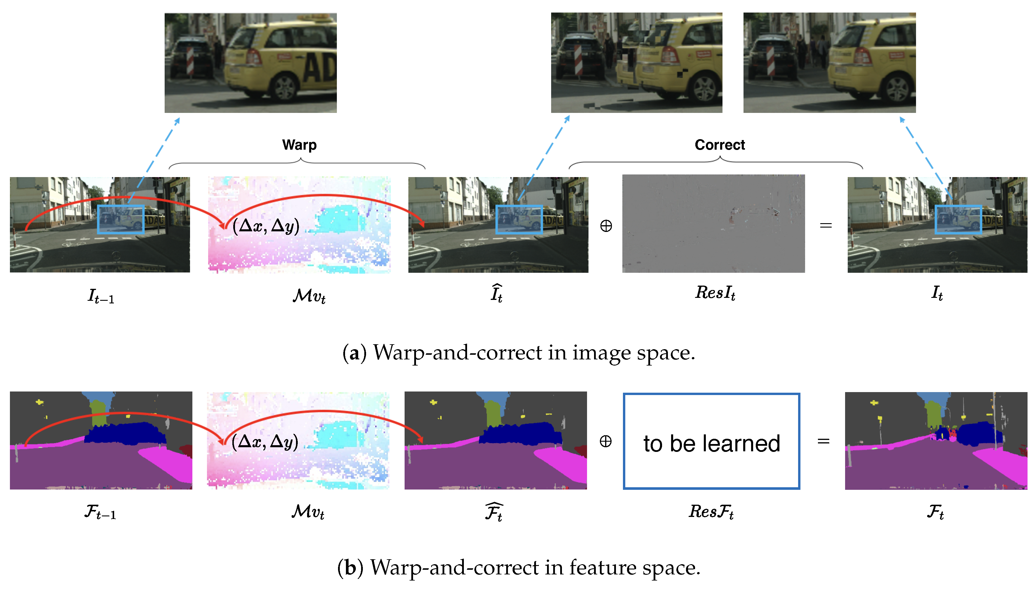
Applsci 13 10102 g001
Figure 2. Illustration of “warp-and-correct”. (a) Video codecs warp the preceding frame to the current one and then add the compressed-domain residuals. (b) We propose to learn the residuals in feature space to rectify the warped features.
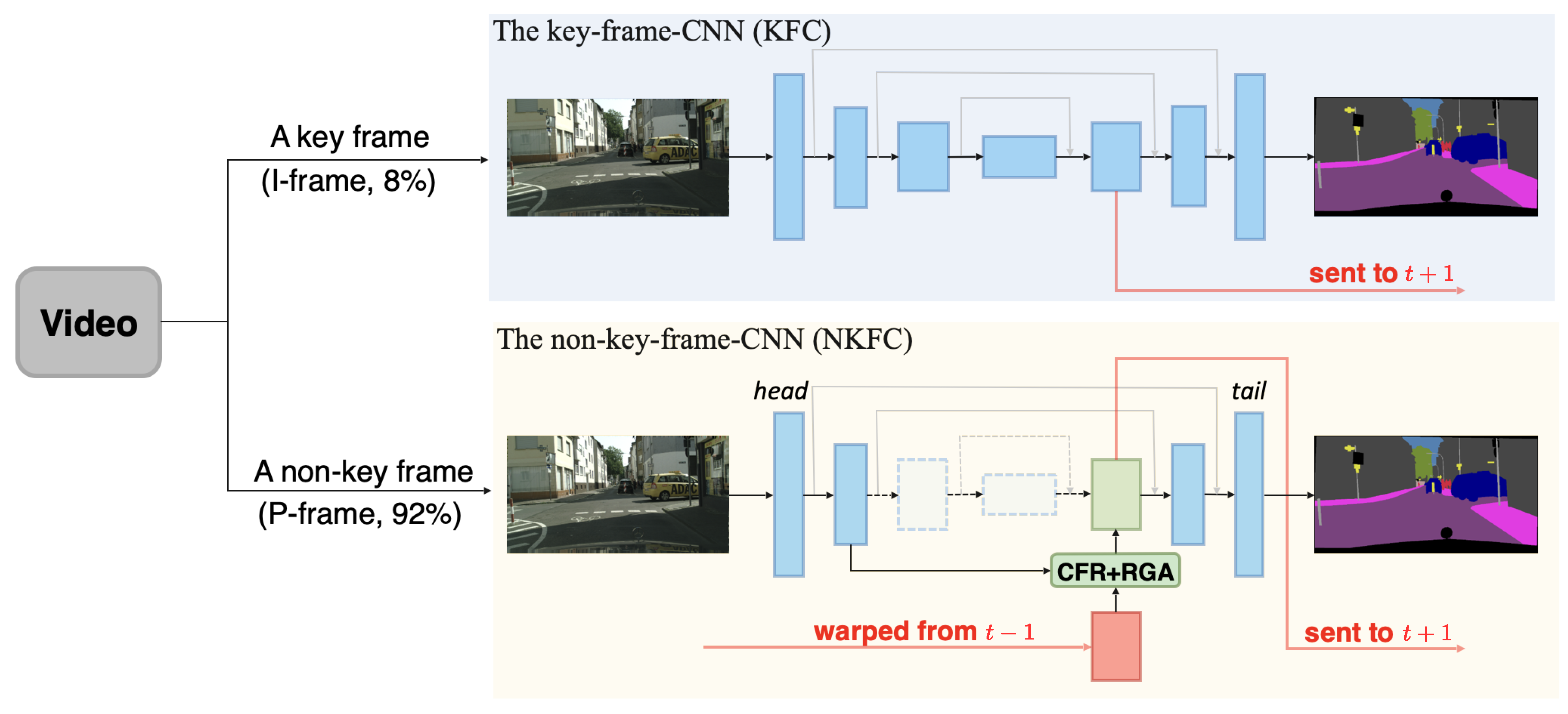
Applsci 13 10102 g002
Figure 3. The framework of TWNet. A group of frames consists of one key frame followed by many non-key frames. Key frames are sent to the key-frame CNN (KFC) and non-key frames to the non-key-frame CNN (NKFC), where the warped context features from the preceding frame are corrected by the CRF and RGA modules. Both CNNs output the result label maps and the interior context feature maps. Dashed arrows and boxes in NKFC indicate the operations to be skipped.
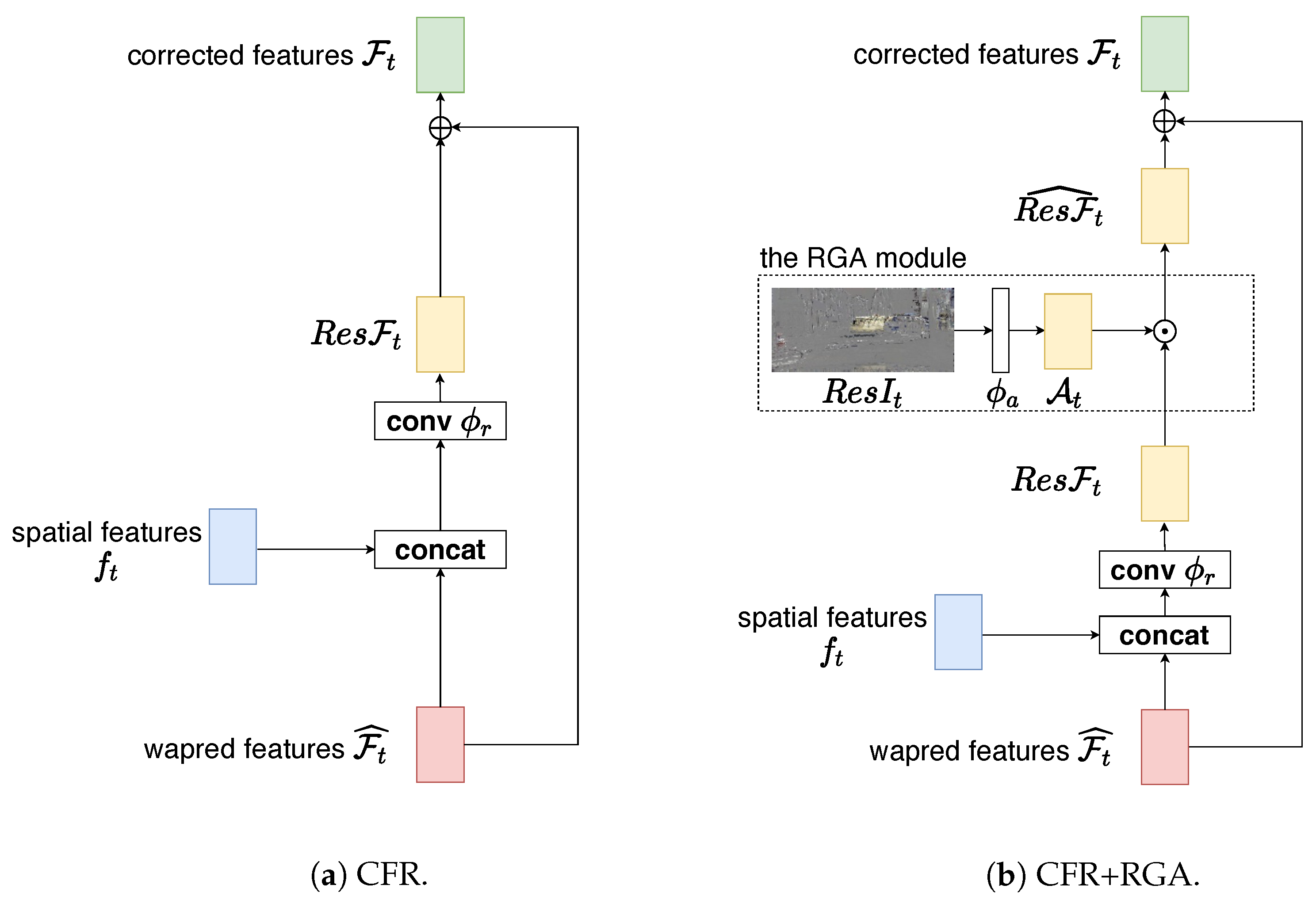
Applsci 13 10102 g003
Figure 4. Illustration of the CFR and RGA modules. (a) The CFR module first concatenates f t , the spatial features of the current non-key frame, and F t ^ , the warped features from the preceding frame. Then, the concatenated features are fed into a convolution layer ϕ r to learn the feature space residuals R e s F t . Finally, CFR adds the R e s F t to F t ^ to obtain the corrected features F t . (b) The RGA module is based on CFR. After obtaining R e s F t , RGA uses compressed domain residuals R e s I t , which are fed into a convolution layer ϕ a to learn the attention map A t . Then, RGA multiplies A t with F t ^ to focus on the error-prone regions and obtains R e s F t ^ . RGA adds R e s F t ^ to F t ^ to obtain the corrected features F t . “⊙”: element-wise multiplication; “⊕”: element-wise addition.
Applsci 13 10102 g004
Figure 5. Choices of different layers for feature warping. The chosen layer is indicated with red color. The dotted arrows and boxes denote skipped operations.
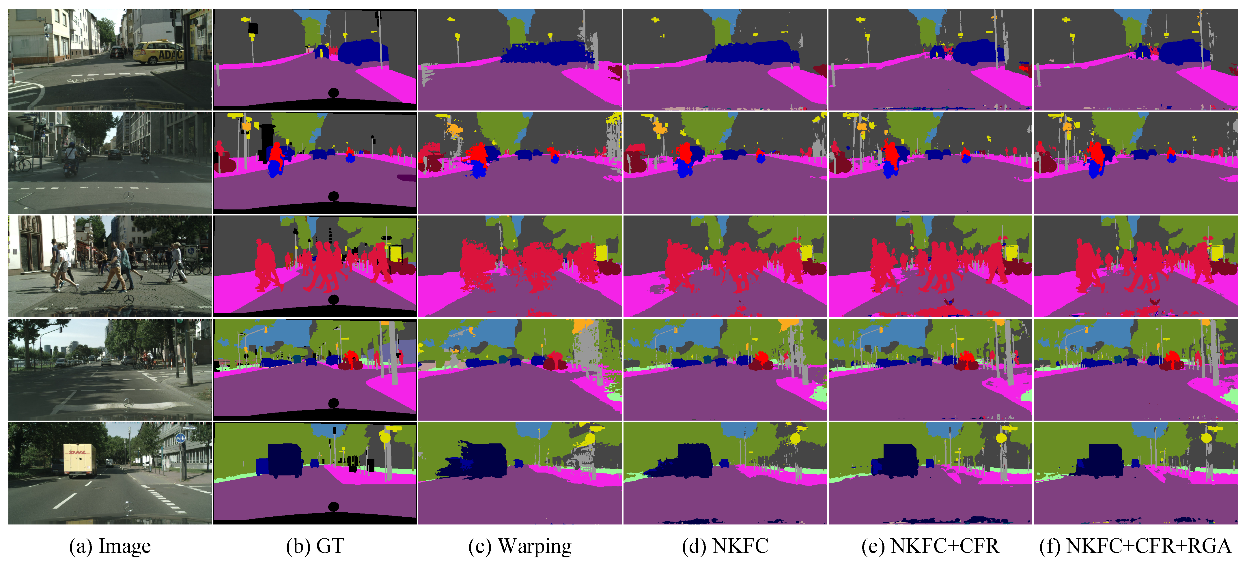
Applsci 13 10102 g005
Figure 6. Qualitative results on Cityscapes. GT: ground truth; warping: normal warping; NKFC: the non-key-frame CNN; CFR: context feature rectification; and RGA: residual-guided attention.
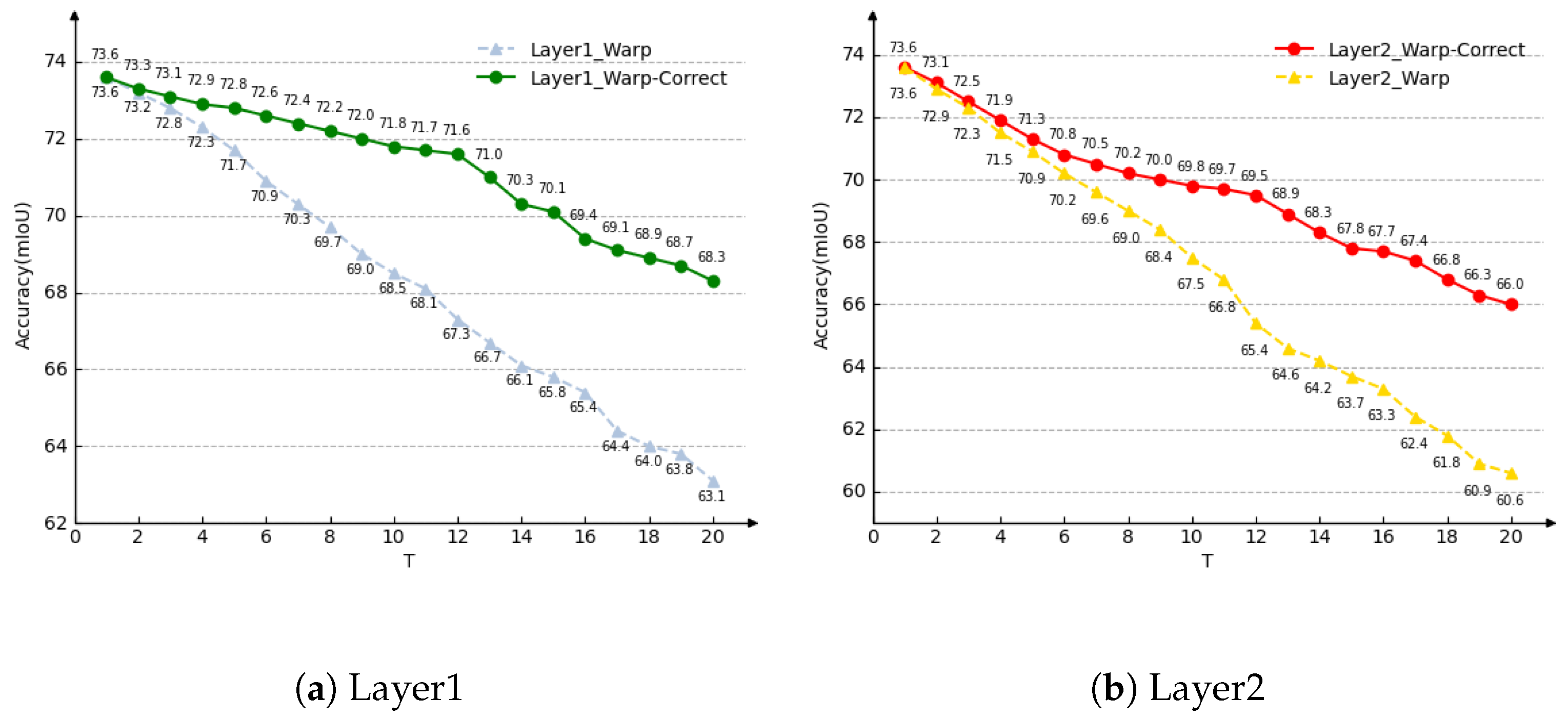
Applsci 13 10102 g006
Figure 7. Performance degradation of warp and warp-correct. (a): Layer 1 used for feature warping. (b): Layer 2 used for warping. T: frame interval between the key frame and the frame to be evaluated. The correction module effectively alleviates the long-term error accumulation problem.
Applsci 13 10102 g007
Table 1. Performance comparison of different layers used for feature warping. “Fine-tuned” indicates whether the second training step is performed to fine-tune NKFC. If not fin-tuned, the parameters of the head and tail layers keep the same as those in KFC. If Layer 3 is chosen, no trainable parameters exist and hence there is no fine-tuning. ↑: higher is better. ✓ indicates the fine-tuning is used. The best results are shown in bold.
Warping LayerFine-TunedmIoU ↑FPS ↑
Layer 1 67.365.5
69.665.5
Layer 2 65.489.8
67.889.8
Layer 3-63.2119.7
Table 2. Validation of L c o n s i s t . λ 1 : the weight of L c o n s i s t . We achieve the bests results when setting λ 1 to 10. ↑: higher is better. The best results are shown in bold.
Warping Layer λ 1 mIoU ↑FPS ↑
Layer 1069.963.1
170.263.1
1070.663.1
2070.363.1
Layer 2067.686.3
168.186.3
1068.686.3
2068.386.3
Table 3. Effect of each module of TWNet. FT: the fine-tuning of the non-key CNN (the second training step); CFR: context feature rectification; and RGA: residual-guided attention. “✓” means the model utilizes the corresponding module. We also show the extra cost of adding our modules. ↑: higher is better; ↓: lower is better. The best results are shown in bold.
Warping LayerFTCFRRGAmIoU ↑FPS ↑GFLOPs ↓
Layer 1. 67.365.5113.28
69.665.5+0
70.663.1+2.42
71.661.8+0.0012
Layer 2. 65.489.873.00
67.889.8+0
68.686.3+2.42
69.584.9+0.0029
Table 4. IoU improvements of different categories. We choose Layer 1 here. The accuracy of non-rigid objects improves significantly. The improvements over five percentage points are shown in bold.
MethodObjectHumanVehicleNatureConstructionSkyFlat
Warping43.856.782.286.687.191.696.6
NKFC 51.2 (+7.4)65.5 (+8.8)84.6 (+2.4)89.6 (+3.0)89.1 (+2.0)94.0 (+2.4)97.3 (+0.7)
NKFC + CFR62.2 (+18.4)75.2 (+18.5)89.7 (+7.5)91.3 (+4.7)90.8 (+3.7)94.2 (+2.6)97.9 (+1.3)
NKFC + CFR + RGA62.2 (+18.4)76.1 (+19.4)90.1 (+7.9)91.1 (4.5)91.0 (+3.9)94.2 (+2.6)98.0 (+1.4)
Table 5. Effect of different flow models. ↑: higher is better. The best results are shown in bold.
Flow ModelmIoU ↑FPS ↑
Motion vectors67.365.5
FlowNet267.513.2
FlowNet2-s66.326.6
FlowNet2-c66.622.7
PWC-Net67.029.4
Table 6. The required head layers for different versions of TWNet. head n: the nth head layer of the encoder. ✓ indicates the specific layer is required.
Model NameHead1Head2Head3
Per-frame
TWNet-Layer1
TWNet-Layer2
TWNet-Layer3
Table 7. Head layers for different backbones. We quote the notations from the TensorFlow Slim package.
BackboneHead1Head2Head3
MobileNetV1 c o n v 2 d _ 3 c o n v 2 d _ 5 c o n v 2 d _ 11
MobileNetV2 l a y e r _ 4 l a y e r _ 7 l a y e r _ 14
ResNet-18 c o n v 2 _ 2 c o n v 3 _ 2 c o n v 4 _ 2
Table 8. Performance of TWNet based on different backbone networks. Warp: the layer where feature warping is performed. “None” means no feature warping. ↑: higher is better. × indicates the speed-up times. The best results are shown in bold.
BackboneWarpmIoU ↑FPS ↑Speed-Up (×)
MobileNetV1None73.635.5-
Layer171.661.81.74
Layer269.584.92.39
Layer363.2119.73.37
MobileNetV2None73.232.3-
Layer171.359.61.85
Layer269.482.52.55
Layer362.4115.83.59
ResNet-18None71.636.9-
Layer169.463.61.72
Layer267.786.82.35
Layer361.9120.43.26
Table 9. Comparison of SOTA models on Cityscapes. Terms with “-pf”: mIoU/FPS for per-frame model; “FPS norm” is calculated based on the ability of the GPU. All the results only use train as the training set. All of the TWNet models run at a resolution of 1024 × 2048 . ↑: higher is better; ↓: lower is better. The best results are shown in bold.
ModelEval SetResolutionmIoU-pf ↑mIoU ↑FPS-pf ↑FPS ↑FPS Norm ↑Params (M) ↓GPU
Per-frame Models
ICNet [22]val 1024 × 2048 67.7-30.3-49.725.17TITAN X(M)
ERFNet [27]test 1024 × 2048 69.7-11.2-18.42.08TITAN X(M)
SwiftNetRN-18 [19]val 1024 × 2048 74.4-34.0-34.012.91080 Ti
CAS [21]val 1024 × 2048 74.0-34.2-48.91070
Liu et al. [23]val 1024 × 2048 73.9-20.8-20.83.21080 Ti
TD-PSP18 [25]val 1024 × 2048 76.8-11.8-10.512.77Titan Xp
DABNet [29]test 512 × 1024 70.1-104.0-104.00.761080 Ti
LRNNet [58]test 512 × 1024 72.2-71.0-71.00.681080 Ti
LEANet [14]test 512 × 1024 71.9-77.3-77.30.741080 Ti
LAANet [13]test 512 × 1024 73.6-95.8-95.80.671080 Ti
DDRNet-23-slim [46]test 1024 × 2048 77.4-101.6-79.375.72080 Ti
Video-based Models
DFF [34]val 512 × 1024 71.169.21.525.612.8N/ATesla K40
DVSNet1 [33]val 1024 × 2048 73.563.25.630.430.442.731080 Ti
DVSNet2 [33]val 1024 × 2048 73.570.45.619.819.862.91080 Ti
Prop-mv [31]val 1024 × 2048 75.261.71.37.69.68.7Tesla K80
Interp-mv [31]val 1024 × 2048 75.266.61.37.29.18.7Tesla K80
Low-Latency [32]val 1024 × 2048 80.275.92.88.4-50.1N/A
LMA [59]val 512 × 1024 72.173.799.086.267.2N/A2080 Ti
Ours
TWNet-Layer1val 1024 × 2048 73.671.635.561.861.812.351080 Ti
TWNet-Layer1test 1024 × 2048 73.171.235.561.861.812.35
TWNet-Layer2val 1024 × 2048 73.669.535.584.984.912.14
TWNet-Layer2test 1024 × 2048 73.169.035.584.984.912.14
Table 10. Effect of each module on the CamVid test set. ↑: higher is better. The best results are shown in bold. ✓ indicates the module is used.
Warping LayerFTCFRRGAmIoU ↑FPS ↑
Layer 1 68.8183.1
69.9183.1
71.0179.8
71.5175.2
Layer 2 66.7252.6
68.1252.6
69.3245.8
70.0240.7
Table 11. Comparison with others on the CamVid test set. ↑: higher is better; ↓: lower is better. The best results are shown in bold.
ModelResolutionmIoU-pf ↑mIoU ↑FPS-pf ↑FPS ↑FPS Norm ↑Params (M) ↓GPU
Per-frame Models
DFANet A [9] 720 × 960 64.7-120-196.87.8TITAN X
ICNet [22] 720 × 960 67.1-27.8-45.625.17TITAN X (M)
BiSeNet [10] 720 × 960 68.7-116.2-103.413.43Titan Xp
BiSeNet V2 [43] 720 × 960 73.2-32.7-32.7491080 Ti
Liu et al. [23] 720 × 960 78.2-27.8-27.83.21080 Ti
TD-PSP18 [25] 720 × 960 72.6-25-22.312.77Ttian Xp
DABNet [29] 360 × 480 66.7-124.4-124.40.761080 Ti
LRNNet [58] 360 × 480 67.6-83.0-83.00.671080 Ti
LEANet [14] 360 × 480 67.5-98.6-98.60.741080 Ti
LAANet [13] 360 × 480 67.9-112.5-112.50.671080 Ti
DRRNet-23-slim [46] 720 × 960 74.3-230-179.75.72080 Ti
Video-based Models
Prov-mv [31] 720 × 960 68.663.43.621.427.08.7Tesla K80
Interp-mv [31] 720 × 960 68.667.33.619.124.18.7Tesla K80
Ours
TWNet-Layer1 720 × 960 73.571.5103.5175.2175.212.351080 Ti
TWNet-Layer2 720 × 960 73.570.0103.5240.7240.712.141080 Ti
Disclaimer/Publisher’s Note: The statements, opinions and data contained in all publications are solely those of the individual author(s) and contributor(s) and not of MDPI and/or the editor(s). MDPI and/or the editor(s) disclaim responsibility for any injury to people or property resulting from any ideas, methods, instructions or products referred to in the content.

