Article

Encoder–Decoder Structure Fusing Depth Information for Outdoor Semantic Segmentation

1
School of Mathematics and Computer Science, Wuhan Polytechnic University, No.36 Huanhu Middle Road, Dongxihu District, Wuhan 430048, China
2
School of Technology, Beijing Forestry University, No.35 Qinghua East Road, Haidian District, Beijing 100083, China
*
Author to whom correspondence should be addressed.
Appl. Sci. 2023, 13(17), 9924; https://doi.org/10.3390/app13179924
Submission received: 25 July 2023 / Revised: 29 August 2023 / Accepted: 31 August 2023 / Published: 1 September 2023
(This article belongs to the Special Issue Advances in Computer Vision and Semantic Segmentation)

Abstract

:
The semantic segmentation of outdoor images is the cornerstone of scene understanding and plays a crucial role in the autonomous navigation of robots. Although RGB–D images can provide additional depth information for improving the performance of semantic segmentation tasks, current state–of–the–art methods directly use ground truth depth maps for depth information fusion, which relies on highly developed and expensive depth sensors. Aiming to solve such a problem, we proposed a self–calibrated RGB-D image semantic segmentation neural network model based on an improved residual network without relying on depth sensors, which utilizes multi-modal information from depth maps predicted with depth estimation models and RGB image fusion for image semantic segmentation to enhance the understanding of a scene. First, we designed a novel convolution neural network (CNN) with an encoding and decoding structure as our semantic segmentation model. The encoder was constructed using IResNet to extract the semantic features of the RGB image and the predicted depth map and then effectively fuse them with the self–calibration fusion structure. The decoder restored the resolution of the output features with a series of successive upsampling structures. Second, we presented a feature pyramid attention mechanism to extract the fused information at multiple scales and obtain features with rich semantic information. The experimental results using the publicly available Cityscapes dataset and collected forest scene images show that our model trained with the estimated depth information can achieve comparable performance to the ground truth depth map in improving the accuracy of the semantic segmentation task and even outperforming some competitive methods.

1. Introduction

Image semantic segmentation plays a critical role in computer vision tasks, an interdisciplinary subject in the fields of machine learning, artificial intelligence and computer vision and involves several computer techniques such as image recognition, image understanding and analysis. High–level semantic labels are assigned to each pixel in an image, that is, each pixel is classified. Semantic segmentation is a fundamental technology for scene understanding and plays a vital role in areas such as autopilot [1], autonomous navigation [2], image medical treatment [3], UAV landing and daily life [4].
Traditional semantic segmentation is mainly used to extract the low–level and intermediate features of images, including segmentation algorithms based on the threshold, region, watershed and graph theory [5,6,7]. With advancements in computing performance, semantic segmentation using machine learning methods began to be included within the research scope of many initiatives. Machine learning methods mainly use traditional classifiers to classify images, which mainly include random decision forests (RF) [8,9] and support vector machines (SVM) [10], but these methods mainly divide data into two categories. The formal application of deep learning in the field of semantic segmentation occurred with the emergence of fully convolutional neural networks (FCN), which can clearly distinguish the categories of objects in an image, such as cats and dogs. FCN can learn pixel–to–pixel mapping, and the size of the input image can be arbitrarily set [11]. This method uses VGG–16 [12] as the basic network to extract features, replaces the fully connected layers with a decoder consisting of deconvolution and convolution for up–sampling, and refines low–resolution feature maps to generate a dense prediction. However, the FCN method has two disadvantages. The first is that the output result is too small, and the spatial features of some pixels are lost in the pooling process. The second is that the context and spatial location information are not fully considered. Cao et al. [13] proposed a new loss, called affinity regression loss (AR loss), to improve the training speed of the semantic segmentation model without relying on contextual information to improve accuracy. Contextual information has been proven to be a powerful clue in semantic segmentation [14,15]. Li et al. [14] suggested that objects with similar appearances are one of the challenges of semantic segmentation tasks. Therefore, they proposed a novel context–based tandem network (CTNet) to mine spatial and channel context information to obtain better semantic segmentation results. Liu et al. [15] argued that continuous down–sampling operations lead to a loss of spatial detail information in the image. Therefore, they proposed a multi–context refinement network (MCRNet) to fuse contextual information for pixel–level semantic segmentation. However, these related methods require the design of additional modules to extract contextual information, which increases the complexity of the model.
Recent related work solved these problems using RGB–D data. The main advantage is attributed to the depth of information in the scene being less affected by illumination and other conditions, which can improve the performance of semantic segmentation tasks. Sun et al. [16] proposed real–time RGB–D fusion semantic segmentation, called RFNet. The model can effectively utilize complementary block modal information to meet the requirements of automatic driving. Hu et al. [17] proposed an attention complementary network (ACNet) that extracts weighted features from RGB images and depth maps, respectively, and fuses them to solve the problem of unequal amounts of information contained in RGB and depth images. Zhou et al. [18] proposed an asymmetric encoder structure for RGB-D indoor scene understanding, which can reduce the difference between low–level and high–level features so as to better fuse features for segmentation. Ying et al. [19] believed that the depth information obtained from sensors is not always reliable, so they proposed the uncertain aware self–attention mechanism to achieve control from unreliable depth information to reliable depth information flow to solve the problem of RGB–D semantic segmentation. Huang et al. [20] proposed a new semantic segmentation solution named LDFNet by fusing brightness, depth and color information. However, current state–of–the–art methods [16,17,18,19,20] still have many problems: (a) relying on expensive depth sensors, such as Microsoft Kinect or 3D LiDAR, to obtain high–quality ground truth depth maps for RGB–D semantic segmentation [21]; (b) simply using depth maps as the fourth channel of RGB images without fully utilizing the complementarity of RGB and depth information (due to the significant differences in features between RGB images and depth maps, it is necessary to fuse depth maps encoded with RGB images [22]); and (c) there are problems such as losing multi–scale information features, which have a great impact on the segmentation accuracy of small objects. If small receptive fields are used to extract the features of small objects, it is difficult to extract global semantic information, and if larger receptive fields are used to extract the background information of images, the features of small targets will be lost. The deep learning method based on multiple scales can combine the deep semantic information and shallow representation information of small objects to solve the problem of feature and position information loss caused by the increase in network layers in small object semantic segmentation [23].
To this end, inspiration from multi–modal joint training can ensure the robustness of semantic segmentation models based on single–modal feature learning [24]. Thus, we improved the semantic segmentation method from the following perspective: a neural network model for image semantic segmentation fused with predicted depth information, which utilizes the multi–modal fusion of RGB and depth images to achieve image semantic segmentation to enhance scene understanding. Specifically, our method is divided into two stages. First, depth estimation of the input RGB images was performed using our previous related work [25,26]. Second, after fusing the predicted depth information with the RGB images, FCNs with encoding and decoding were further used to implement semantic labeling of the outdoor scenes. The overall contribution of our research is summarized below:
(1) The raw RGB image and the predicted depth image were fused into a four–channel RGB–D image using self–calibrating fusion architecture and then an encoding–decoding model was established to output the predicted semantic image;
(2) We proposed a new feature pyramid attention structure, which integrates the fused information at multiple scales to obtain features with rich semantic information;
(3) Our method was evaluated using the publicly available Cityscapes dataset [27] and achieved comparable performance to the ground truth depth map, performing even better than some competitive methods. Furthermore, our method was generalized according to two different forest scenes to demonstrate its effectiveness.
The rest of this paper is arranged as follows: the image semantic segmentation network model and detailed implementation process are outlined in Section 2; the experimental comparison and analysis are shown in Section 3; and finally, the conclusions and recommendations for future works are given in Section 4.

2. Materials and Methods

Image semantic segmentation is an important basis for understanding a scene, and the final segmentation images are formed by assigning different labels to different categories of objects. At present, a deep neural network is widely used in the field of semantic segmentation; however, continuous convolution and pooling operations reduce the resolution of the image [15], which causes the output feature maps and the original image to not have a point–to–point correspondence. Therefore, the traditional deep neural network model has been unable to effectively complete a high–precision semantic segmentation task.
The rich geometric cues contained in the depth map can be used as supplementary information to improve the semantic segmentation accuracy of RGB images [14]. In most circumstances, the cost of acquiring a ground truth depth map in real–world scenarios is expensive, limiting the massive growth of datasets. Therefore, we proposed a new semantic segmentation model that fuses depth information from a depth estimation model without relying on depth sensors. First, we fused the RGB images with predicted depth maps and then input them into a semantic segmentation model to achieve accurate segmentation of RGB images. To this end, we showed the overall structure of the RGB–D image semantic segmentation neural networks and described each module in detail. Second, we introduced data augmentation methods to improve the generalizability and robustness of our semantic segmentation model. Third, we used a cross–entropy function in the field of semantic segmentation as the loss function to measure the difference between the real and predicted probability distributions.

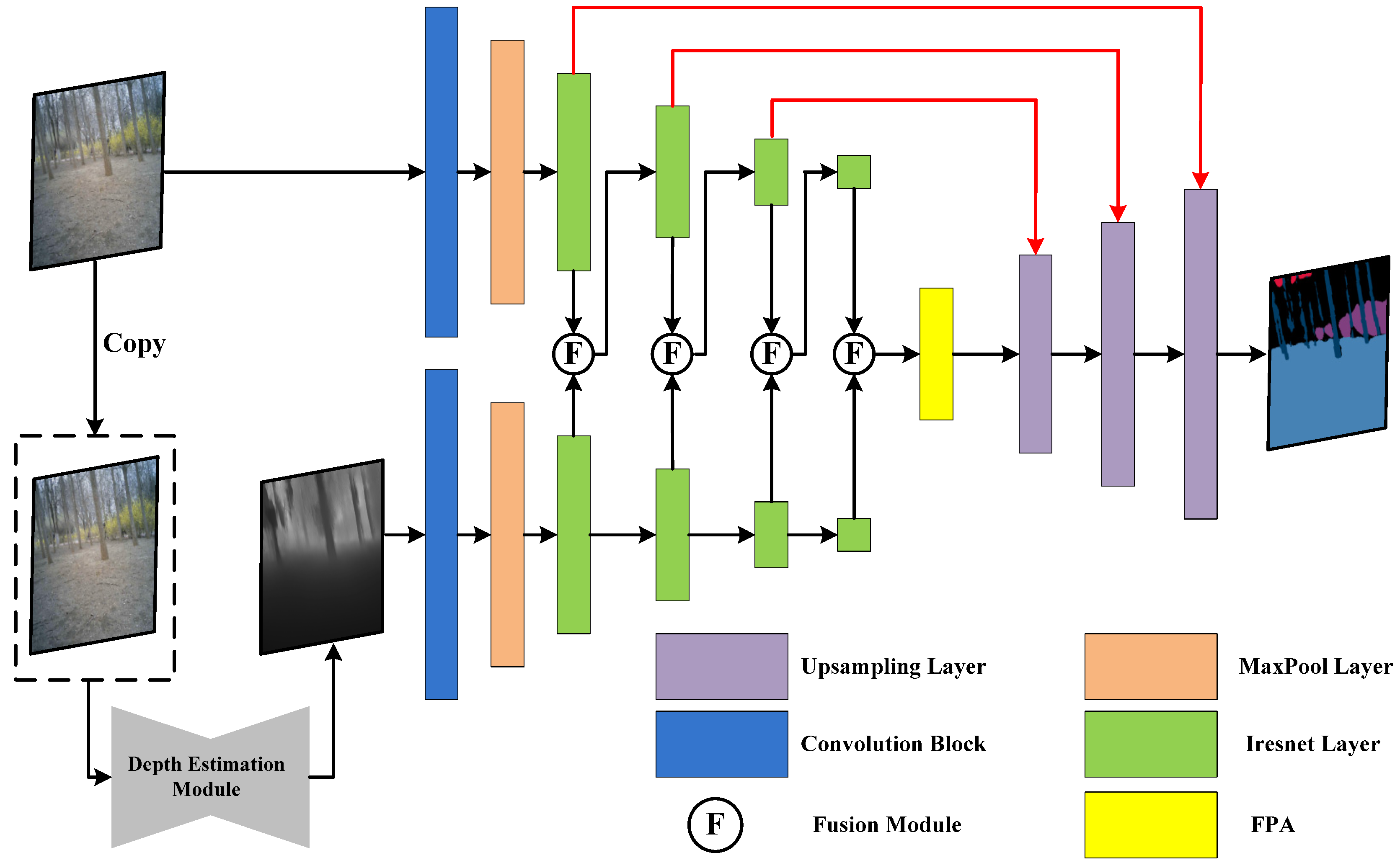
2.1. Semantic Segmentation Model

We mainly investigated the expansion of color images with the corresponding predicted depth in improving the performance of semantic segmentation. The learning–based depth estimation method is divided into two domains: supervised and unsupervised learning methods. The depth estimation models used in this paper originate from our previous related work [25,26]. Figure 1 outlines a summary of our semantic segmentation model with an encoding−decoding structure fusing depth information. For the encoder, the representative features of the RGB and predicted depth images were automatically extracted using our backbone network model, which was based on the improved residual network—IResNet [28]. The effective fusion of image and depth information was implemented as the input of the next layer followed by a fusion module. For the decoder, a series of up–sampling structures were used to gradually restore the resolution of the output feature map. The feature pyramid attention (FPA) network builds a bridge between the encoder and decoder modules, which mainly extracts multiscale information from the features output by the encoder module as the input to the decoder module. Some shortcut connections (red arrows) were also added between the corresponding layers in the encoder and decoder to enhance the information flow.

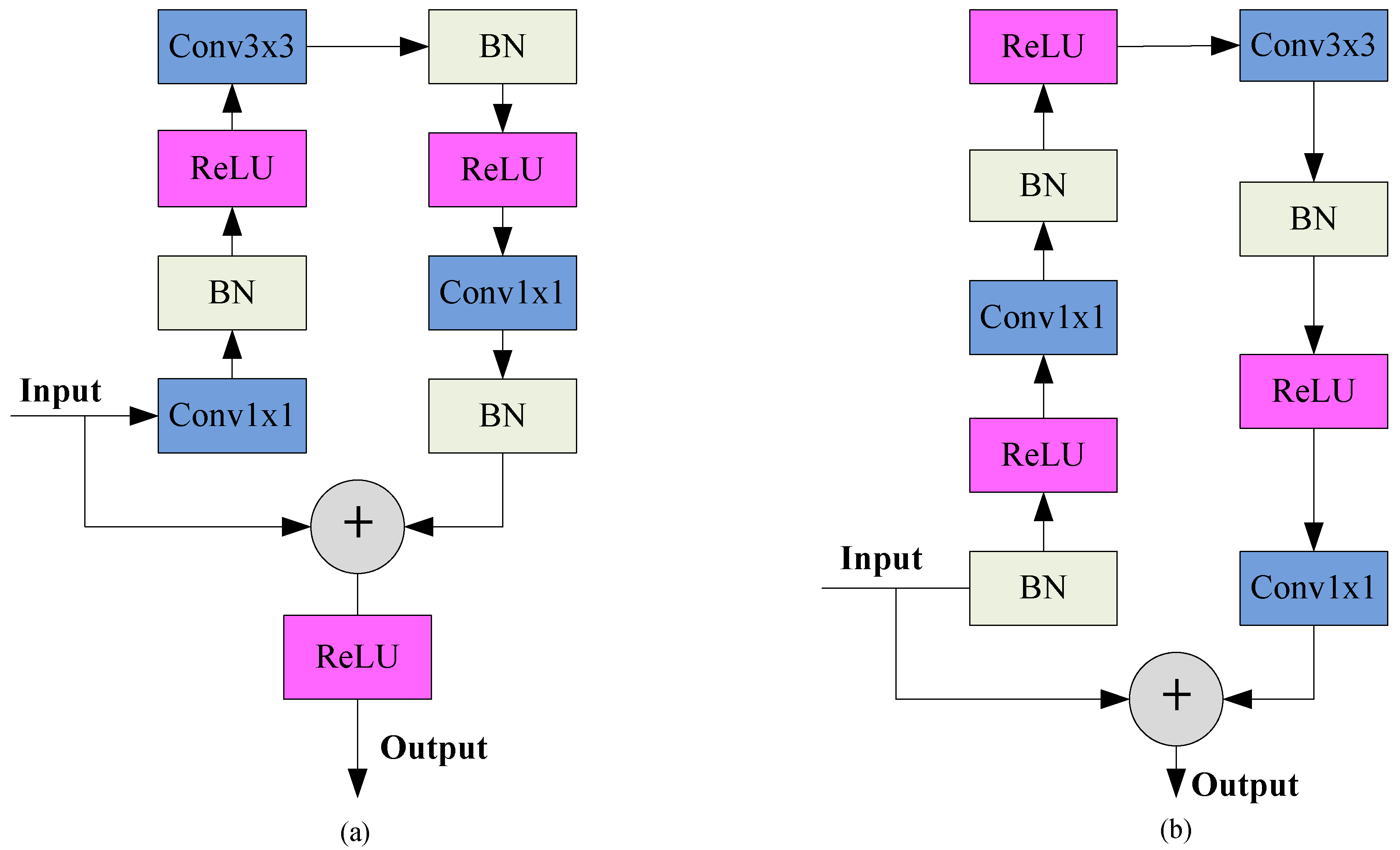
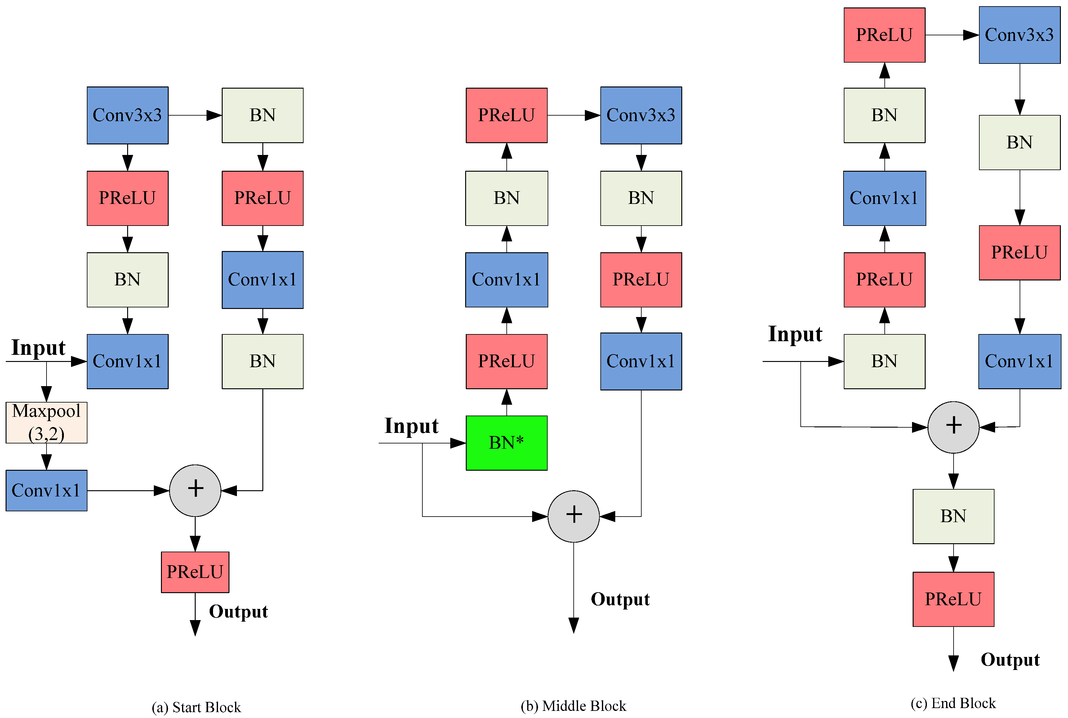
2.1.1. The Encoder Module

The backbone network of the encoder module was mainly composed of improved residual blocks, which improved the raw residual block and the preactivated residual block [29], as shown in Figure 2.
Conv1×1 and Conv3×3 were the convolution operations with kernel sizes of 1 × 1 and 3 × 3, respectively. BN represents batch normalization (BN), and the rectified linear unit (ReLU) was the activation function. The raw residual block was added a ReLU function to the main path to return the negative signal to zero. However, in the early stage of convolutional neural network (CNN) training, there may have been more negative signals that may have had a negative impact on information propagation. To solve this problem, a preactivation residual block was proposed. The BN and ReLU functions were placed before the convolution operator, and the feature map was directly output after Conv1×1, which led to a lack of nonlinear characteristics between the modules and limited the learning ability of the CNN. In addition, the raw residual and preactivation residual blocks were not added to be the BN function on the main path, which also means that the feature maps added channel–by–channel were not normalized, increasing the difficulty of CNN training.
We proposed an improved residual network structure as the backbone network for semantic segmentation, which is mainly divided into three parts: the start block, middle block and end block, as shown in Figure 3.
BN* indicates that the BN was not added to the first middle block because the BN function is already included in the auxiliary path of the start block. Maxpool (3, 2) is a 3 × 3 max pooling layer with a stride of 2. For the nonlinear activation function, we used the parametric rectified linear unit (PReLU) [30] to replace ReLU.
ResNet was the first choice for the semantic segmentation tasks [31,32,33,34]. In the process of training ResNet, stochastic dropping of hidden nodes or connection layers (the most common is the dropout method [35]) did not affect the convergence of the algorithm, showing that ResNet had good redundancy. We used an improved ResNet, called IResNet, which contains the start, main and end stages. There are four main stages, including three, four, six and three blocks, respectively. Each main stage includes a start block and an end block, and the rest are middle blocks. The entire IResNet network only contains the activation function PReLU [30] in the main path of the end block in the main stage, which reduces the adverse effects of the nonlinear function in information propagation and makes use of the advantages of nonlinear mapping. At the same time, the network adds a regularization term to the main path of the end block to regularize the output features added channel–by–channel. The end block of each main stage is connected with the start block of the next stage. The auxiliary path of the start block plus the regularization term and the main path parameters are added channel–by–channel to normalize all the features. Adding regularization items and activation functions to the main path of the end block can stabilize the signal entering the next stage, which is in preparation for the next stage of feature processing. The network can effectively control the flow of information without increasing the network parameters and only changing the layout.
When the scales of the input and output features in the start block do not match, a down–sampling operation needs to be added to the main path to maintain the same scale as adding by the channel. ResNet–50 [29] uses a 1 × 1 convolution with a stride of 2 to adjust the scale of the feature map. However, the 1 × 1 convolution with a stride of 2 will cause a significant loss of information and introduce noise, which will have a negative impact on the main path information. A 3 × 3 max pooling layer with a stride of 2 was used in IResNet–50 to change the size of the feature map, which helped select the most active elements for retention, and a convolution operation was used to change the number of channels. The 3 × 3 convolution operation in the auxiliary path adjusted the feature map to help preserve the spatial context. The max pooling kernel was the same as the convolution kernel in the auxiliary path to ensure that the channel–wise addition was performed between the elements computed in the same window. This operation does not add any other parameters to the model.

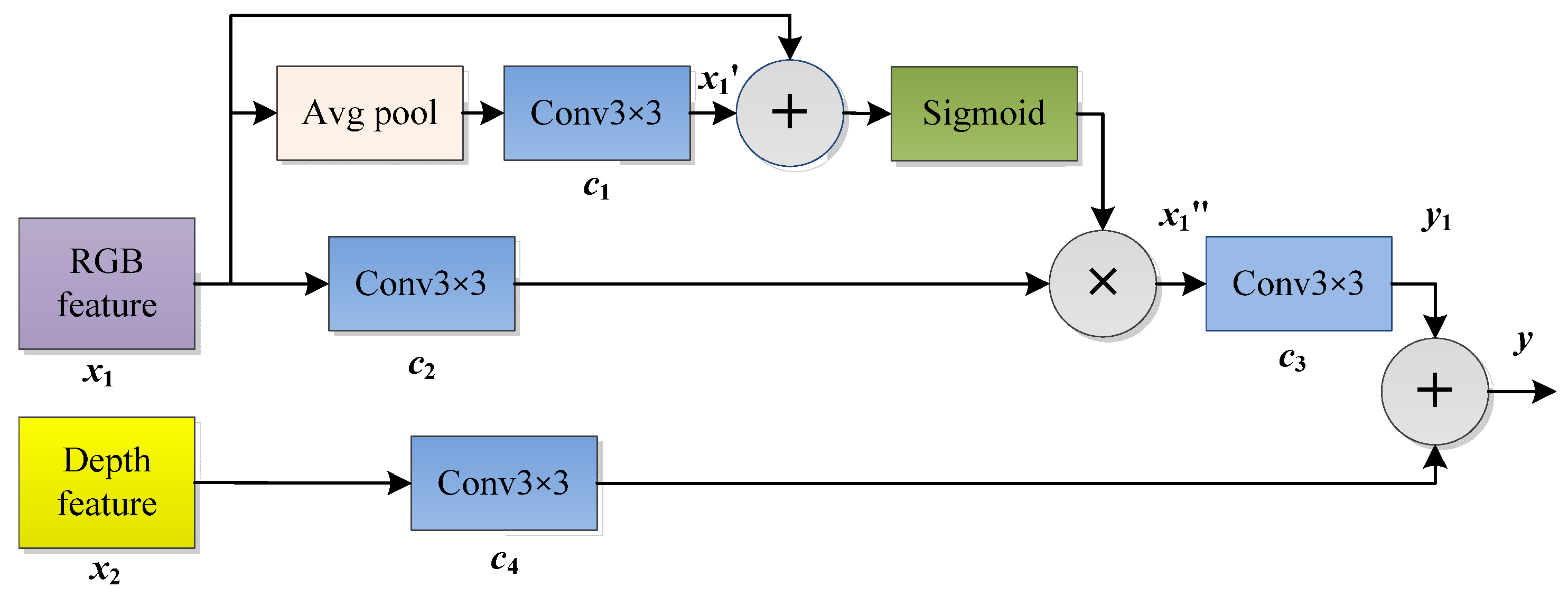
2.1.2. Self–Calibrating Fusion Architecture

The depth map contained more contour and position information, which is helpful for RGB image semantic segmentation [16,17]. Identifying ways that can effectively utilize depth information complementary to RGB images to promote semantic segmentation accuracy is an important research hotspot in the field of RGB–D image semantic segmentation. We proposed a self–calibration module (Figure 4) to learn fusion information from an RGB image and predicted depth maps. The self–calibration module can enhance the diversity of the output features by expanding the size of the receptive field.
In the figure, Avg pool represents the global average pooling operation; Cov3×3 is the 3 × 3 convolutional layer; “+” and “×” represent channel–by–channel addition and multiplication, respectively; x 1 , x 1 and y 1 are the output features of the intermediate layers; and y is the final output of the fusion structure.
When general convolution is used for feature extraction of spatial locations, the size of the receptive field is set to a fixed size, resulting in the inability to extract higher–level semantic information. To extract the effective context information of each spatial location, our proposed self–calibration fusion structure fused the image and depth features to achieve self–calibration of the RGB image features and then added them with a channels–wise deep map. Each branch in the self–calibrated fusion structure nonuniformly divided the convolution filter into multiple parts, and the filters of each part were used in a heterogeneous form. The specific execution process is as follows:
{ T 1 = a v g   p o o l ( x 1 ) x 1 = u p ( c 1 ( T 1 ) ) x 1 = c 2 ( x 1 ) · σ ( x 1 + x 1 ) y 1 = c 3 ( x 1 ) y = c 4 ( x 2 ) + y 1 .
where up is the up–sampling operation and σ (   ) is a sigmoid function.
First, the RGB image was down–sampled using a 3 × 3 average pooling layer to obtain T1 (see Equation (1)) and then bilinear interpolation was used to restore T1 to the size of x 1 , which was added with input x 1 to obtain the attention feature map of the spatial domain. After processing the sigmoid activation function, the output features were multiplied channel–by–channel with the feature map after a c 2 transformation to obtain feature map x 1 , which was finally output as y 1 using a 3 × 3 convolutional layer. The self–calibrating operation described above allows each spatial location to adaptively treat its surrounding information environment as an embedding from the low–resolution latent space and also model the dependence between the channels. Therefore, the receptive field of self–calibrating convolution can be effectively expanded.

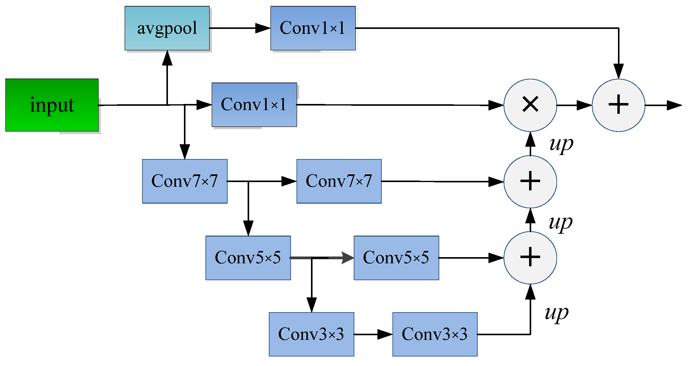
2.1.3. Feature Pyramid Attention Mechanism

Although the pyramid structure [33] can extract multiscale feature information and effectively increase the size of the receptive field, it lacks global context prior attention and cannot select features in the dimension direction. On the other hand, the channel–based attention mechanism is not sufficient to extract multiscale features effectively, lacking pixel–level information [23]. To increase the size of the receptive field and improve the segmentation accuracy of small objects, we fused the attention mechanism and spatial pyramid structure to construct the FPA mechanism and extract accurate and dense multiscale features. We also used the convolution kernels of different scales (3 × 3, 5 × 5 and 7 × 7) to extract the contextual information of the input feature map, and the FPA structure to fuse the features of different scales layer–by–layer. After the 1 × 1 convolution layer, the original features were multiplied by the multiscale features pixel–by–pixel to efficiently capture the context information of the multiscale image. The specific structure of the FPA module is shown in Figure 5.
After the 3 × 3 convolution operation, the size of the output feature map was 1/8 of the input feature. In the figure, “up” is the deconvolution operation, the purpose of which is to increase the scale of the feature map for channel–by–channel fusions with high–resolution features. The 1 × 1 convolution on the main path was used to reduce the number of channels. High–level features were not conducive to pixel–level classification, so we performed average pooling of the high–level features, which then underwent a 1 × 1 convolutional layer to obtain a 1 × 1 × C vector with global information to weight the channels of the low–level features. The context features of different scales can be fused with the FPA module to expand the feature representation range of advanced feature maps. The context information was multiplied with the original feature map pixel–by–pixel without introducing excessive computation.

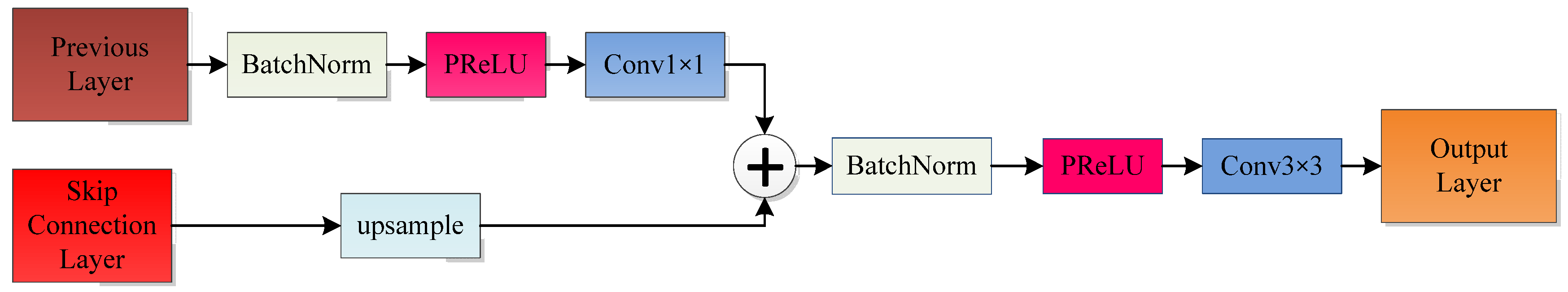
2.1.4. The Decoder Module

The function of the decoder module was to gradually restore the resolution of the output feature map, including three up–sampling structures, the detailed structure of which is shown in Figure 6. Inspired by ReNet [29], we used skip connections to take the input features (the red arrow in Figure 1) and the output features from the previous layer as inputs to our up–sampling structure so that the model could learn the residual and avoid the loss of information. We applied a 1 × 1 convolution operation and a bilinear interpolation operation on the two branches, with the upper branch containing a BN layer and a PReLU [30] layer. Finally, we summed the results of the two branches and output the feature map through a BN layer, a PReLU layer and a 3 × 3 convolutional layer. We must clarify that the third up–sampling module in the decoding module was different from the first two, mainly using four–time interpolation to keep the same size of the input RGB images as the output semantic segmentation result.

2.2. Data Augmentation

A large quantity of training data was a prerequisite for achieving an accurate model. To improve the generalizability and robustness of our semantic segmentation model, we transformed the training data using random operations performed spontaneously. The augmentation methods are described as follows [25,26]:
  • Random horizontal flip. Input images and the target ground truth are both horizontally flipped with a 0.5 probability.
  • Random rotation. Input images and the target ground truth are both rotated with a random value.
  • Scale. Input images and the target ground truth are both scaled by a random number u ∈ [0.5, 2].
  • Random crop. Input images and the target ground truth are both center–cropped and then restored to the original size.

2.3. Loss Function

We applied the most commonly used cross–entropy function in the field of semantic segmentation as the loss function, which was used to measure the difference between the real and predicted probability distributions [16,17]. The segmentation problem can be viewed as a multiclassification problem. Therefore, similar to the classification task, we used the sigmoid function to output a probability value representing the probability of a positive sample at the last layer of the semantic segmentation model. The probability that the network outputs positive samples is:
y = P ( y = 1 | x )
The probability of outputting negative samples is:
1 y = P ( y = 0 | x )
From the perspective of maximum likelihood, we integrated Equations (2) and (3) to obtain
P ( y | x ) = ( y ) y ( 1 y ) 1 y
To avoid changing the monotonicity of Equation (4), we took the logarithms at both ends of Equation (4):
log P ( y | x ) = log ( y y ( 1 y ) 1 y ) = y log y + ( 1 y ) log ( 1 y ) .
The greater the probability of the positive samples, the higher the accuracy of object segmentation in the foreground. Finally, we obtained the cross–entropy equation as follows:
L = 1 N i = 1 N y ( i ) log y ( i ) + ( 1 y ( i ) ) log ( 1 y ( i ) ) .
For the multiobjective segmentation problem, the cross–entropy loss function can be expressed as [18,19,20]:
L = c = 1 M o = 1 N y o , c log ( p o , c )
where N is the total number of pixels, o is a pixel index, M is the total number of categories, y o , c is the probability that ground truth pixel o belongs to category c, and the value is 0 or 1, and p o , c is the probability that pixel o is predicted to be true category c, which is the output of the semantic segmentation model.

3. Experimentation

In this section, we evaluate our method based on the common metrics and protocols used for prior methods and compare them with existing semantic segmentation approaches. Since this paper mainly addresses the semantic segmentation of outdoor scenes, we used the publicly available Cityscapes dataset [27] as a benchmark to train our model. The dataset is commonly used to evaluate semantic segmentation performance for outdoor scenes. In addition, we conducted relevant experiments in real forest scenes to further demonstrate the effectiveness of our approach. Our method was implemented using the PyTorch [36] framework, which is a machine learning toolkit released by Facebook that can run on GPUs to achieve acceleration.

3.1. Brief Overview of Depth Estimation Methods

The depth estimation methods used in this paper were derived from our previous research results [25,26]. We mainly used two different schemes to train the depth estimation model. The first scheme uses a supervised learning approach, and since the training dataset contains RGB images and corresponding depth images, we proposed an encoder–decoder structure with the feature pyramid to predict the depth map from a single RGB image [25]. The second scheme uses an unsupervised learning method. Since the training dataset only contains rectified stereo pairs without corresponding depth images, we considered the depth prediction problem as a regression problem of the disparity map based on the basic principle of binocular stereo vision [26].

3.2. Training Dataset

We conducted related experiments on the autonomous driving outdoor dataset, Cityscapes, which is large in scale and covers 50 cities in Germany and nearby countries, including street scenes in the spring, summer and autumn, and is widely used in RGB–D semantic segmentation research. It contains 5000 densely annotated images, which are officially divided into 2975 training sets, 500 validation sets and 1525 testing sets. The resolution of the images is 2048 × 1024. The finely annotated objects in this dataset can be divided into 19 categories, including road, sidewalk, building, wall, fence, pole, traffic light, traffic sign, vegetation, terrain, sky, pedestrian, rider, car, truck, bus, train, motorbike and bicycles. This dataset does not provide the ground truth segmentation images of the test set, so we use the validation set as the test set to test the experimental effect of the network model.

3.3. Training Details

We trained the semantic segmentation model on 2975 training data using the Adam [37] optimizer with a batch size of 4 and set the learning rate to be 1 × 10⁻⁴. In addition, we used a polynomial decay strategy to adjust the learning rate of the model, and the formula is as follows:
l r = r ( 1 t T ) p o w e r
where l r is the current learning rate, r is the initial learning rate, which is set to 1 × 10⁻⁴, power is the attenuation coefficient, generally set to 0.9, t is the number of current iterations and T is the maximum number of iterations. Due to the limitations of the semi–global matching algorithm, the left and bottom halves of the depth images are not applicable, so these pixels needed to be cropped, and bilinear interpolation up–sampling was used to adjust the image to the original resolution. To accelerate the training, the input images were down–sampled to 768 × 768 to remove the blank boundaries or invalid regions caused by data augmentation. Our semantic segmentation model was trained on one NVIDIA Titan Xp GPU for approximately 200 epochs.
We show the detailed visual results of the Cityscapes datasets in Figure 7. We found that our method was more accurate in the segmentation of large target objects such as cars, trees, and buildings, and worked well in the segmentation of smaller object categories such as billboards and poles.

3.4. Evaluation Criteria

The evaluation criteria are an important basis for a quantitative evaluation of the model performance. For the image semantic segmentation task, there are several categories:
I.
Pixel accuracy (PA): P A = i = 0 k p i i i = 0 k j = 0 k p i j ,
II.
Intersection over union (IoU): I o U = i = 0 k p i i j = 0 k p i j + i = 0 k p j i p i i ,
III.
Mean intersection over union (mIoU):
m I o U = 1 k + 1 i = 0 k p i i j = 0 k p i j + i = 0 k p j i p i i ,
IV.
Frequency weighted intersection over union(FWIoU):
F W I o U = 1 k + 1 i = 0 k p i i j = 0 k p i j + i = 0 k p j i p i i .
where k is the total number of categories, p i i indicates that the predicted category is i and the real category is also i and p i j indicates that the predicted category is j and the real category is i.
To verify the segmentation effect of our method using different objects within the Cityscapes dataset, we first reported the classification results of the different objects on the IoU. Then, we compared the IoU performance of our method with other classical semantic segmentation algorithms using different targets in detail. Finally, the comprehensive performance of our method was compared with that of classical semantic segmentation algorithms in detail to systematically illustrate the segmentation effect of our method.

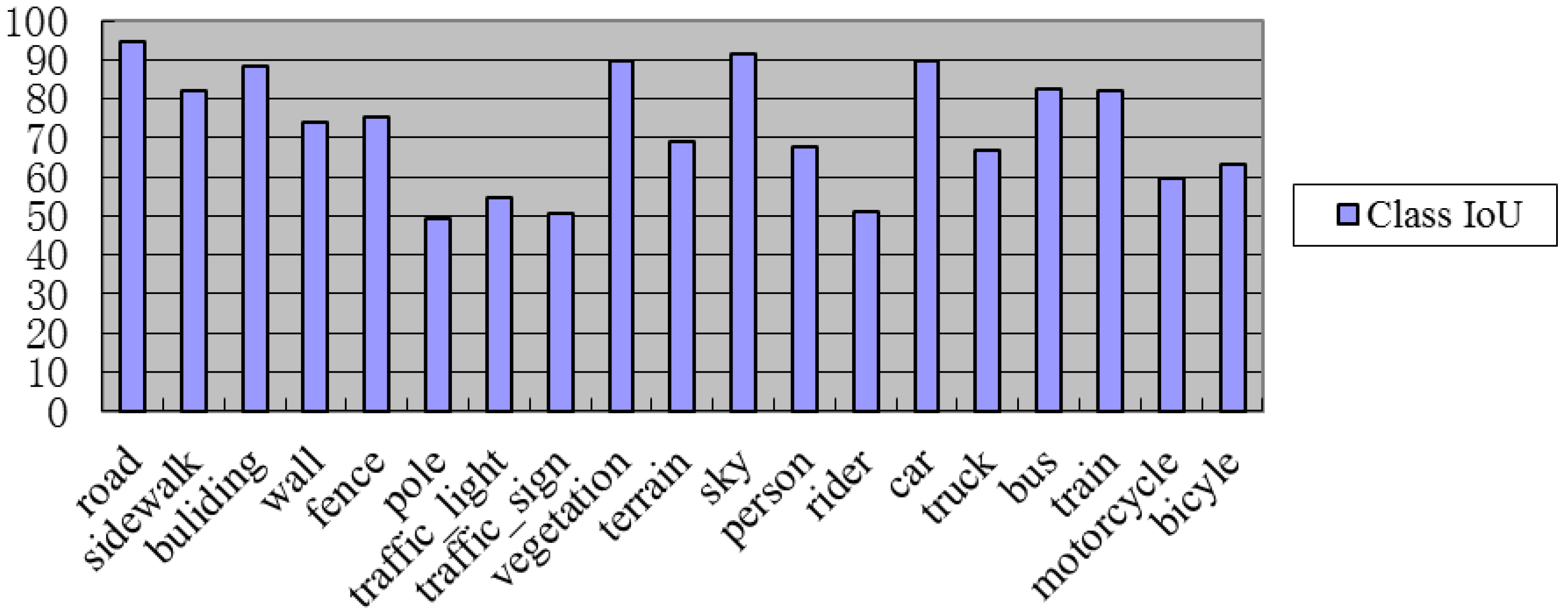
3.4.1. IoU Results for Different Object Classifications within the Cityscapes Dataset

Figure 8 shows the detailed IoU results for different object classifications within the Cityscapes dataset. The IoU results are close to 90%, and more than 90% have five categories, namely, road, building, vehicle, sky and car. This shows that the segmentation method is effective in large target segmentations. The object categories with IoU results of more than 80% include the sidewalk, bus and train. More than 70% of the object categories have walls and fences, indicating that these objects achieved good segmentation results. However, the segmentation effect for terrain, person, truck, motorcycle and bicycle was general, and the IoU of the other objects was less than 60%. The main reason is that the Cityscape dataset was mainly captured using corresponding sensors installed on autonomous driving devices. This means that the image contained more categories, such as the sky, road and cars, and fewer categories such as poles, traffic lights and bicycles. The final mIoU of our method was approximately 73%.
Table 1 summarizes the IoU results of our method on different objects. Our method significantly outperformed SwiftNet [38] and RFNet [16] on the sidewalk, wall, fence, terrain and train categories and could achieve comparable performance on the road, vegetation, sky and bus categories.

3.4.2. mIoU Results for the Cityscapes Dataset

Table 2 summarizes the comparison of our results with results obtained using other semantic segmentation methods. Compared with the segmentation algorithms without fusion depth information, our method had a higher mIoU, more accurate segmentation results and a good overall performance. At the same time, we also concluded that semantic segmentation results with estimated depth information could achieve comparable performance for the ground truth depth map and even outperformed some competitive methods. In addition, the PA and FWIoU of our method were 93.1% and 87.9%, respectively.
Although the fusion of RGB images and depth maps with the self–calibrating fusion architecture and feature pyramid attention mechanism raised the computational cost, our semantic segmentation model ran at an average speed of 10.43 FPS (frames per second) on a single Nvidia Titan Xp Gpu for input images with a quantity of 1525 and size of 768 × 768. Training approximately 200 epochs on 2975 training sets, the trainable parameters were about 444.9 M. Overall, our multimodal semantic segmentation method incorporating predicted depth information achieved the best results while maintaining real–time performance, which also demonstrated that utilizing predicted depth information could improve the efficiency of semantic segmentation.

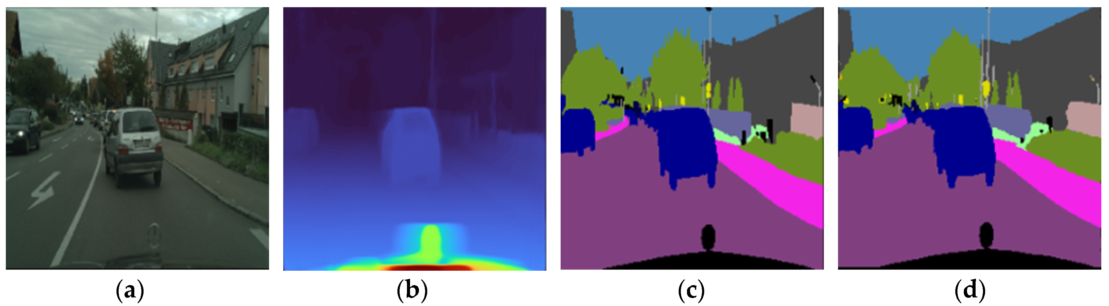
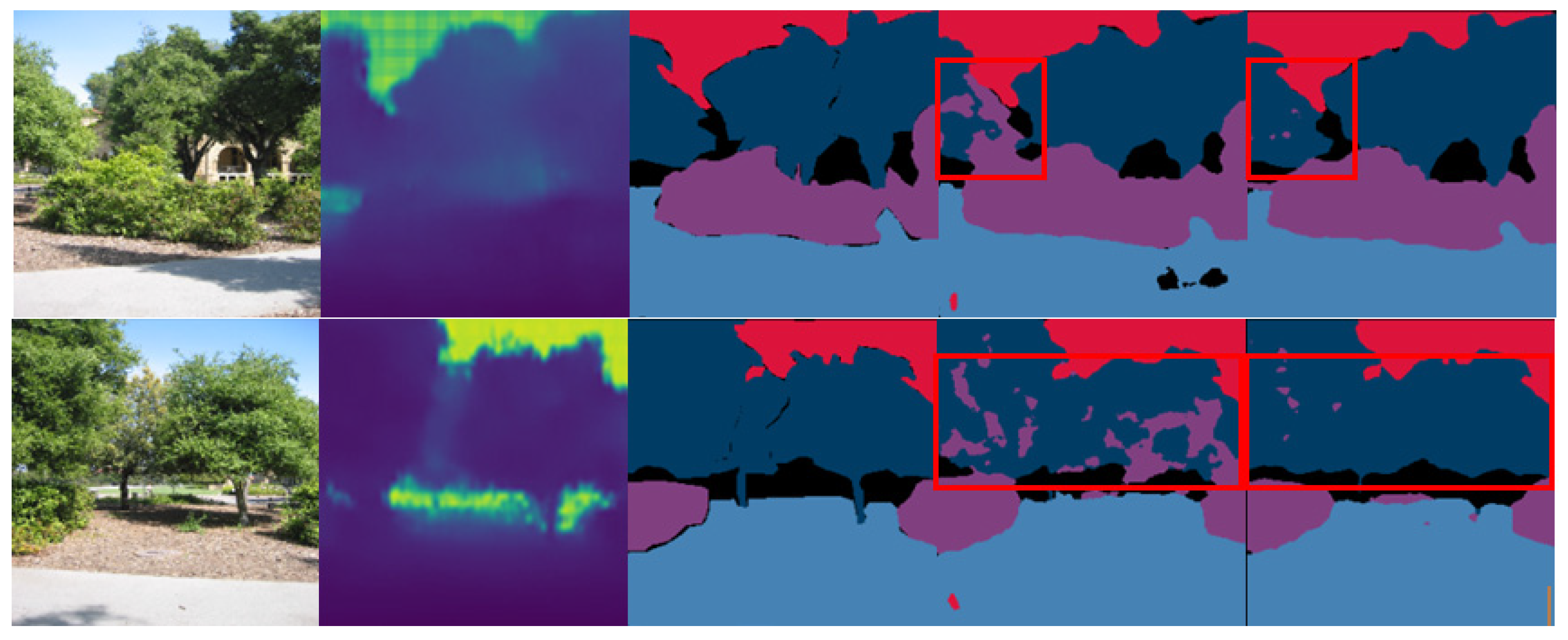
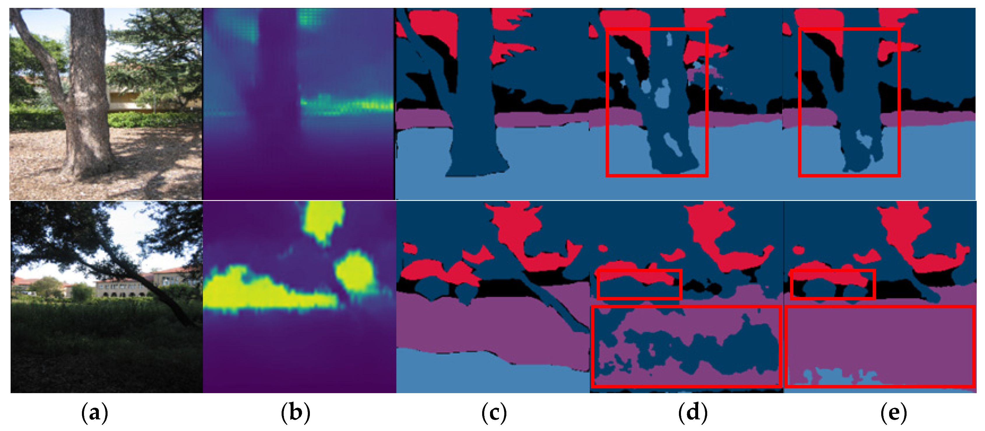
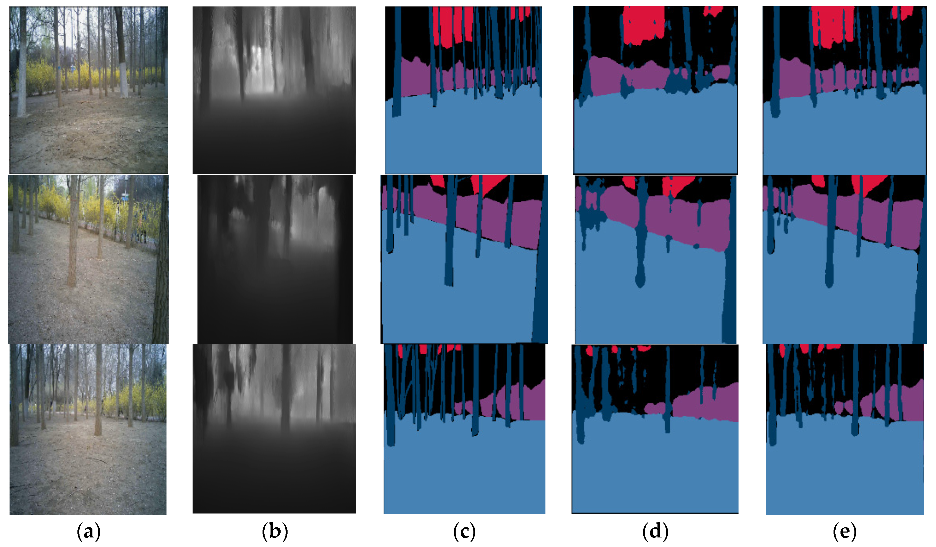
3.5. Experimental Results for the Forest Scene

We also conducted related experiments using two different forest scenes, which further demonstrated the effectiveness of our method. We first used the image labeling tool—labelme to manually label the forest images in the Make3D [43] dataset. The images were mainly divided into four categories, namely, blue trees, red sky, purple bushes and black background. A previous related work [25] was then used to predict the depth map of the forest image. Finally, the depth and RGB images were fused as the input for the semantic segmentation network.
First, we conducted experiments using a public dataset containing images of the forest areas, and the detailed experimental results are shown in Figure 9. From Figure 9d,e, it can be seen that the result of semantic segmentations without depth information fusion produced large errors, while the segmentation results with depth information fusion were more accurate. In the area marked with the red box in the fourth row of Figure 9, a distant tree could be segmented using the RGB–D semantic segmentation network model.
Second, we conducted experiments using 1k forestry images collected at the Beijing Olympic Forest Park. In fact, there were many trees in the forest scene, with a small DBH (diameter at breast height) and light color, and the branches were blocked from each other. When manually labeling, we only labeled the trunks in the foreground and divided the branches and trees in the background into the background without labeling. The experimental results are shown in Figure 10. The accuracy of our method for real forest scene segmentations was higher than that of the model without depth information.
Furthermore, we evaluated our method using two different forest datasets since previous related works [11,39,40,41] did not provide evaluation results on forest scenes. In order to compare fairly with relevant methods, we used the work by Hu et al. [17] and our method to evaluate the results using the two different forest datasets. Table 3 shows a comparison of the results.

4. Conclusions

In this paper, we proposed a self–calibrating RGB–D semantic segmentation neural network model based on an improved residual network for the semantic segmentation of multimodal information. First, we used IResNet [6] to extract features from RGB and predicted depth images. Then, our designed self–calibration network performed multimodal fusion of the depth information and RGB image features and utilized the feature pyramid attention structure to fuse multiscale semantic information. Finally, we presented a bilinear interpolation structure as a decoder module to generate segmentation results with high resolution and rich semantic information. The experimental results for the publicly available Cityscapes dataset [27] and collected forest scene images show that our method outperformed the competitive methods.
Our model trained with the estimated depth information could achieve comparable performance to the ground truth depth map in improving the accuracy of the semantic segmentation task. However, the reasoning process of our semantic segmentation was divided into two parts; that is, it first predicted the depth map and then performed3semantic segmentation. Although our method improved the prediction accuracy, it also correspondingly increased the time of single image segmentation. Second, the fusion of RGB images and depth images with the self–calibrating fusion architecture and feature pyramid attention mechanism increased the computational cost of the model.
In future work, we will focus on semantic segmentation of 3D objects to solve fundamental problems such as unmanned driving, smart healthcare and 3D object recognition.

Author Contributions

S.C.: writing—original draft, methodology, visualization, investigation, validation and formal analysis. M.T.: methodology, writing—review and editing, conceptualization, supervision and funding acquisition. R.D. and J.K.: supervision, methodology and writing—review and editing. All authors have read and agreed to the published version of the manuscript.

Funding

This work was funded by the National Natural Science Foundation of China (Grant number 32071680); the Science and Technology Fund of Henan Province (Grant number 222102110189); Research and Innovation Initiatives of WHPU; and research funding from Wuhan Polytechnic University (Grant number 2023Y46). The authors gratefully acknowledge this support.

Data Availability Statement

The data are available from the corresponding author upon request.

Acknowledgments

This research was sponsored by Wuhan Polytechnic University and Beijing Forestry University. The authors gratefully acknowledge this support.

Conflicts of Interest

The authors declare no conflict of interest.

References

  1. Xu, Y.; Wang, H.; Liu, X.; He, H.R.; Gu, Q.; Sun, W. Learning to See the Hidden Part of the Vehicle in the Autopilot Scene. Electronics 2019, 8, 331. [Google Scholar] [CrossRef]
  2. Fusic, S.J.; Hariharan, K.; Sitharthan, R. Scene terrain classification for autonomous vehicle navigation based on semantic segmentation method. Trans. Inst. Meas. Control 2022, 44, 2574–2587. [Google Scholar] [CrossRef]
  3. Karri, M.; Annavarapu, C.S.R.; Acharya, U.R. Explainable multi–module semantic guided attention based network for medical image segmentation. Comput. Biol. Med. 2022, 151, 106231. [Google Scholar] [CrossRef] [PubMed]
  4. Yi, S.; Li, J.J.; Jiang, G. CCTseg: A cascade composite transformer semantic segmentation network for UAV visual perception. Measurement 2022, 151, 106231. [Google Scholar]
  5. Otsu, N. A threshold selection method from gray–level histograms. IEEE Trans. Syst. Man Cybern. 1979, 9, 62–66. [Google Scholar] [CrossRef]
  6. Cong, S.P.; Sun, J.Z. Application of Watershed Algorithm for Segmenting Overlapping Cells in Microscopic Image. J. Image Graph. 2016, 103, 3505–3511. [Google Scholar]
  7. Shi, J.; Malik, J.M. Normalized cuts and image segmentation. IEEE Trans. Pattern Anal. Mach. Intell. 2000, 22, 888–905. [Google Scholar]
  8. AI–Awar, B.; Awad, M.M.; Jarlan, L.; Courault, D. Evaluation of Nonparametric Machine–Learning Algorithms for an Optimal Crop Classification Using Big Data Reduction Strategy. Remote Sens. Earth Syst. Sci. 2022, 5, 141–153. [Google Scholar]
  9. Jozwicki, D.; Sharma, P.; Mann, I.; Hoppe, U.P. Segmentation of PMSE Data Using Random Forests. Remote Sens. 2022, 14, 2976. [Google Scholar] [CrossRef]
  10. Sarker, I.H. Machine Learning: Algorithms, Real–World Applications and Research Directions. SN Comput. Sci. 2021, 2, 160. [Google Scholar] [CrossRef]
  11. Long, J.; Shelhamer, E.; Darrell, T. Fully Convolutional Networks for Semantic Segmentation. IEEE Trans. Pattern Anal. Mach. Intell. 2015, 39, 640–651. [Google Scholar]
  12. Simonyan, K.; Zisserman, A. Very deep Convolutional networks for large–scale image recognition. arXiv 2014, arXiv:1409.1556. [Google Scholar]
  13. Cao, L.M.; Yang, Z.W. Use square root affinity to regress labels in semantic segmentation. arXiv 2021, arXiv:2103.04990. [Google Scholar]
  14. Li, Z.; Sun, Y.; Zhang, L.; Tang, J. CTNet: Context–Based Tandem Network for Semantic Segmentation. IEEE Trans. Pattern Anal. Mach. Intell. 2021, 44, 9904–9917. [Google Scholar] [CrossRef] [PubMed]
  15. Lin, Q.; Dong, Y.S.; Li, X.L. Multi–stage context refinement network for semantic segmentation. Neurocomputing 2023, 535, 53–63. [Google Scholar]
  16. Sun, L.; Yang, K.; Hu, X.; Hu, W.; Wang, K. Real–Time Fusion Network for RGB–D Semantic Segmentation Incorporating Unexpected Obstacle Detection for Road–Driving Images. IEEE Robot. Autom. Lett. 2020, 5, 5558–5565. [Google Scholar] [CrossRef]
  17. Hu, X.X.; Yang, K.L.; Fei, L. ACNET: Attention Based Network to Exploit Complementary Features for RGBD Semantic Segmentation. In Proceedings of the IEEE International Conference on Image Processing (ICIP), Taipei, Taiwan, 22–25 September 2019; pp. 1440–1444. [Google Scholar]
  18. Zhou, W.; Lv, S.; Lei, J.; Luo, T.; Yu, L. RFNet: Reverse Fusion Network with Attention Mechanism for RGB–D Indoor Scene Understanding. IEEE Trans. Emerg. Top. Comput. Intell. 2023, 7, 598–603. [Google Scholar] [CrossRef]
  19. Ying, X.W.; Chuah, M.C. UCTNet: Uncertainty–Aware Cross–Modal Transformer Network for Indoor RGB–D Semantic Segmentation. In Proceedings of the European Conference on Computer Vision (ECCV), Tel Aviv, Israel, 23–27 October 2022; pp. 20–37. [Google Scholar]
  20. Hung, S.W.; Lo, S.Y.; Hang, H.M. Incorporating Luminance, Depth and Color Information by a Fusion–Based Network for Semantic Segmentation. In Proceedings of the IEEE International Conference on Image Processing (ICIP), Taipei, Taiwan, 22–25 September 2019; pp. 2374–2378. [Google Scholar]
  21. Liu, F.; Shen, C.; Lin, G.; Reid, I. Learning Depth from Single Monocular Images Using Deep Convolutional Neural Fields. IEEE Trans. Pattern Anal. Mach. Intell. 2016, 38, 2024–2039. [Google Scholar] [CrossRef]
  22. Li, X.; Li, L.; Alexander, L.; Wang, W.; Wang, X. RGB–D object recognition algorithm based on improved double stream convolution recursive neural network. Opto–Electron. Eng. 2021, 48, 200069. [Google Scholar]
  23. Ge, Y.; Chen, Z.-M.; Zhang, G.; Heidari, A.; Chen, H.; Teng, S. Unsupervised domain adaptation via style adaptation and boundary enhancement for medical semantic segmentation. Neurocomputing 2023, 550, 126469. [Google Scholar] [CrossRef]
  24. Du, C.; Teng, J.; Li, T.; Liu, Y.; Yuan, T.; Wang, Y.; Yuan, Y.; Zhao, H. On Uni–Modal Feature Learning in Supervised Multi–Modal Learning. arXiv 2023, arXiv:2305.01233. [Google Scholar]
  25. Tang, M.X.; Chen, S.N.; Kan, J.M. Encoder–Decoder Structure with the Feature Pyramid for Depth Estimation from a Single Image. IEEE Access 2021, 9, 22640–22650. [Google Scholar] [CrossRef]
  26. Chen, S.N.; Tang, M.X.; Kan, J.M. Monocular Image Depth Prediction without Depth Sensors: An Unsupervised Learning Method. Appl. Soft Comput. 2020, 97, 106804. [Google Scholar] [CrossRef]
  27. Cordts, M.; Omran, M.; Ramos, S.; Rehfeld, T.; Enzweiler, M.; Benenson, R.; Franke, U.; Roth, S.; Schiele, B. The Cityscapes Dataset for Semantic Urban Scene Understanding. In Proceedings of the 2016 IEEE Conference on Computer Vision and Pattern Recognition (CVPR), Las Vegas, NV, USA, 27–30 June 2016; pp. 3213–3223. [Google Scholar]
  28. Duta, I.C.; Liu, L.; Zhu, F.; Shao, L. Improved Residual Networks for Image and Video Recognition. arXiv 2020, arXiv:2004.04989. [Google Scholar]
  29. He, K.; Zhang, X.; Ren, S.; Sun, J. Deep Residual Learning for Image Recognition. In Proceedings of the 2016 IEEE Conference on Computer Vision and Pattern Recognition (CVPR), Las Vegas, NV, USA, 27–30 June 2016; pp. 770–778. [Google Scholar]
  30. He, K.; Zhang, X.; Ren, S.; Sun, J. Delving Deep into Rectifiers: Surpassing Human-Level Performance on ImageNet Classification. In Proceedings of the 2015 IEEE International Conference on Computer Vision (ICCV), Santiago, Chile, 7–13 December 2015; pp. 1026–1034. [Google Scholar]
  31. Lin, G.; Milan, A.; Shen, C.; Reid, I. RefineNet: Multi–path Refinement Networks for High–Resolution Semantic Segmentation. In Proceedings of the 2017 IEEE Conference on Computer Vision and Pattern Recognition (CVPR), Honolulu, HI, USA, 21–26 July 2017; pp. 5168–5177. [Google Scholar]
  32. Badrinarayanan, V.; Kendall, A.; Cipolla, R. SegNet: A Deep Convolutional Encoder–Decoder Architecture for Image Segmentation. IEEE Trans. Pattern Anal. Mach. Intell. 2017, 39, 2481–2495. [Google Scholar] [CrossRef] [PubMed]
  33. Zhao, H.; Shi, J.; Qi, X.; Wang, X.; Jia, J. Pyramid Scene Parsing Network. In Proceedings of the 2017 IEEE Conference on Computer Vision and Pattern Recognition (CVPR), Honolulu, HI, USA, 21–26 July 2017; pp. 6230–6239. [Google Scholar]
  34. Peng, C.; Zhang, X.; Yu, G.; Luo, G.; Sun, J. Large Kernel Matters—Improve Semantic Segmentation by Global Convolutional Network. In Proceedings of the 2017 IEEE Conference on Computer Vision and Pattern Recognition (CVPR), Honolulu, HI, USA, 21–26 July 2017; pp. 1743–1751. [Google Scholar]
  35. Srivastava, N.; Hinton, G.; Krizhevsky, A.; Sutskever, I.; Salakhutdinov, R. Dropout: A Simple Way to Prevent Neural Networks from Overfitting. J. Mach. Learn. Res. 2014, 15, 1929–1958. [Google Scholar]
  36. Paszke, A.; Gross, S.; Massa, F.; Lerer, A.; Bradbury, J.; Chanan, G.; Killeen, T.; Lin, Z.; Gimelshein, N.; Antiga, L.; et al. PyTorch: An imperative style, high–performance deep learning library. In Proceedings of the International Conference on Neural Information Processing Systems (NIPS), Vancouver, BC, Canada, 8–14 December 2019; pp. 8024–8035. [Google Scholar]
  37. Kingma, D.; Ba, J. Adam: A method for stochastic optimization. arXiv 2014, arXiv:1412.6980. [Google Scholar]
  38. Oršic, M.; Krešo, I.; Bevandic, P.; Segvic, S. In Defense of Pre-Trained ImageNet Architectures for Real–Time Semantic Segmentation of Road–Driving Images. In Proceedings of the 2019 IEEE/CVF Conference on Computer Vision and Pattern Recognition (CVPR), Long Beach, CA, USA, 15–20 June 2019; pp. 12599–12608. [Google Scholar]
  39. Chen, L.-C.; Papandreou, G.; Kokkinos, I.; Murphy, K.; Yuille, A.L. DeepLab: Semantic Image Segmentation with Deep Convolutional Nets, Atrous Convolution, and Fully Connected CRFs. IEEE Trans. Pattern Anal. Mach. Intell. 2018, 40, 834–848. [Google Scholar] [CrossRef]
  40. Paszke, A.; Chaurasia, A.; Kim, S. Enet: A deep neural network architecture for real–time semantic segmentation. arXiv 2016, arXiv:1606.02147. [Google Scholar]
  41. Romera, E.; Alvarez, J.M.; Bergasa, L.M. Erfnet: Efficient residual factorized convnet for real–time semantic segmentation. IEEE Trans. Intell. Transp. Syst. 2017, 19, 263–272. [Google Scholar] [CrossRef]
  42. He, L.; Lu, J.; Wang, G.; Song, S.; Zhou, J. SOSD–Net: Joint semantic object segmentation and depth estimation from monocular images. Neurocomputing 2021, 440, 251–263. [Google Scholar] [CrossRef]
  43. Saxena, A.; Sun, M.; Ng, A.Y. Make3D: Learning 3D Scene Structure from a Single Still Image. IEEE Trans. Pattern Anal. Mach. Intell. 2009, 31, 824–840. [Google Scholar] [CrossRef] [PubMed]
Figure 1. The overall structure of RGB–D image semantic segmentation neural networks.
Applsci 13 09924 g001
Figure 2. The raw residual block and preactivated residual block. (a) Raw residual block and (b) preactivated residual block.
Applsci 13 09924 g002
Figure 3. The residual block in the IResNet network. (a) Start block, (b) middle block and (c) end block.
Applsci 13 09924 g003
Figure 4. Self–calibrating fusion structure.
Applsci 13 09924 g004
Figure 5. Feature pyramid attention structure.
Applsci 13 09924 g005
Figure 6. Our up–sampling structure. We used skip connections to take the input features and the output features from the previous layer as inputs to our up–sampling structure.
Applsci 13 09924 g006
Figure 7. Qualitative results of our approach using the Cityscapes dataset. (a) RGB images; (b) predicted depth map by [26]; (c) ground truth semantic segmentation images; and (d) our result. Note that the brightness of the colors in the depth maps represents the distance of the camera to the object.
Applsci 13 09924 g007aApplsci 13 09924 g007b
Figure 8. The IoU results for different object classifications with the Cityscapes dataset.
Applsci 13 09924 g008
Figure 9. The visual effect on a public dataset containing images of forest scenes. (a) Input images; (b) predicted depth maps by [25]; (c) ground truth images; (d) results without fused depth information; and (e) our approach.
Applsci 13 09924 g009aApplsci 13 09924 g009b
Figure 10. The visual effect on an actual forest scene. (a) Input images; (b) predicted depth maps by [26]; (c) ground truth images; (d) results without fused depth information; (e) our approach.
Applsci 13 09924 g010
Table 1. Comparison of the proposed method with other semantic segmentation methods using different objects.
MethodSwiftNet [38]RFNet [16]Our Method
Road94.996.194.8
Sidewalk54.961.682.3
Wall47.356.974.1
Fence57.760.475.3
Vegetation90.891.189.7
Terrain57.157.169.1
Sky91.991.891.7
Bus80.683.482.4
Train60.473.982.0
Table 2. The comparison of our results with results obtained using other methods for the Cityscapes dataset. “N” denotes methods without fusion depth information, “G” denotes methods with ground truth depth information and “P” denotes methods with predicted depth information.
NetworkRGB–DmIoU
FCN8s [11]N65.3%
DeepLabV2–CRF [39]N70.4%
ENet [40]N58.3%
ERFNet [41]N65.8%
ERF–PSPNet [41]N64.1%
SwiftNet [38]N70.4%
ARLoss [13]N71.0%
LDFNet [20]G68.48%
RFNet [16]G72.5%
ESOSD–Net [42]P68.2%
Our methodP73.0%
Table 3. Baseline comparison of the two forest datasets. Performance evaluation by Hu et al. [17] and our method using the two datasets. P denotes the public dataset containing images of forest areas and M denotes the images collected at the Beijing Olympic Forest Park.
MethodDatasetRGB–DmIoUPA
Hu et al. [17]PYes69.87%93.67%
YYes71.17%94.42%
Our methodPYes73.94%96.95%
YYes75.11%97.45%
Disclaimer/Publisher’s Note: The statements, opinions and data contained in all publications are solely those of the individual author(s) and contributor(s) and not of MDPI and/or the editor(s). MDPI and/or the editor(s) disclaim responsibility for any injury to people or property resulting from any ideas, methods, instructions or products referred to in the content.

