
Contextual Explanations for Decision Support in Predictive Maintenance


Department of Computer Networks and Systems, Silesian University of Technology, Akademicka 16, 44-100 Gliwice, Poland
Appl. Sci. 2023, 13(18), 10068; https://doi.org/10.3390/app131810068
Submission received: 4 August 2023
/
Revised: 30 August 2023
/
Accepted: 5 September 2023
/
Published: 6 September 2023
(This article belongs to the Special Issue Symbolic Methods of Machine Learning in Knowledge Discovery and Explainable Artificial Intelligence)
Abstract
:Explainable artificial intelligence (XAI) methods aim to explain to the user on what basis the model makes decisions. Unfortunately, general-purpose approaches that are independent of the types of data, model used and the level of sophistication of the user are not always able to make model decisions more comprehensible. An example of such a problem, which is considered in this paper, is a predictive maintenance task where a model identifying outliers in time series is applied. Typical explanations of the model’s decisions, which present the importance of the attributes, are not sufficient to support the user for such a task. Within the framework of this work, a visualisation and analysis of the context of local explanations presenting attribute importance are proposed. Two types of context for explanations are considered: local and global. They extend the information provided by typical explanations and offer the user greater insight into the validity of the alarms triggered by the model. Evaluation of the proposed context was performed on two time series representations: basic and extended. For the extended representation, an aggregation of explanations was used to make them more intuitive for the user. The results show the usefulness of the proposed context, particularly for the basic data representation. However, for the extended representation, the aggregation of explanations used is sometimes insufficient to provide a clear explanatory context. Therefore, the explanation using simplification with a surrogate model on basic data representation was proposed as a solution. The obtained results can be valuable for developers of decision support systems for predictive maintenance.
1. Introduction
Explainable artificial intelligence (XAI) methods aim to elucidate the decision-making processes of artificial intelligence (AI) for end users [1]. Consequently, AI systems should be better understood by their developers, more trustworthy for end users and should meet the legal requirements that pertain to them [2]. Research on explainable artificial intelligence has significantly intensified in recent years due to the development of advanced machine learning (ML) techniques and the growing demand for transparency in AI solutions. As a result, XAI methods are increasingly finding applications in various fields. These applications span from medical systems [3,4,5] and service-oriented systems [6] to industrial solutions [7,8]. XAI methods can be classified into two categories: those that generate explanations at the level of the entire data set (global), and approaches that provide explanations for individual data instances (local) [9]. Global explanations focus on a machine learning model as a whole and tend to explain its average behaviour, whereas local explanations focus on a single prediction or recommendation to explain what drove the model to make such a decision [10].
Understanding the range of XAI solutions and their possible applications, it is important to take into account the needs of the end user and the specifics of the data being analysed. For example, global explanations are of grater interest to data scientists creating and evaluating the model, while local explanations are more interesting for the end user who is affected by a particular model decision. In some cases, in addition to a single explanation it may be helpful to consider the broader context of the analysis to properly assess the situation. The necessity to consider explanation context can arise from both the data type and the predictive model used. This means that the development of decision support systems with explainable artificial intelligence methods requires a multi-dimensional analysis of user needs and requirements, and the analytical solutions used.
The motivation for this study comes from prior research [11] on a predictive maintenance task. Predictive maintenance (PdM) aims to prevent unexpected machine failures by identifying deteriorating machine condition and scheduling maintenance in advance. While preventive servicing can effectively avert failures, the absence of failures can pose a challenge for data-driven analytical approaches. To train a machine learning model capable of predicting machine state the proper representations of both “alarm” and “correct operation” classes are required. The solution is to use the anomaly identification (outlier detection) method. In this case, alarms indicating machine malfunctions stem from the anomalies identified in the measurements. Whether the reported alarms indicate a failure must be decided by the operator based on their experience and domain knowledge. The operator’s judgment can be augmented by local explanations, which are generated for a single data point and show the importance of the attributes on which the model made its decision. Such explanations can guide the operator towards specific machine components that behave abnormally, e.g., if sensor readings for a particular component are the most important for the model’s anomaly detection decision. Typically, however, the XAI methods used do not support the operator in identifying false alarms. In addition, the model’s decisions may be based on derived attributes, which provide the operator with limited insight.
The objective of this study is to propose and assess extensions to the local explanations of PdM model decisions. This research assumes that the model relies on outlier detection and processes multivariate time series. The proposed solution uses the temporal characteristics of data and has the form of a context for local explanations. Thus, it aligns with the concept of human-centred explanations by considering the context for a given data point instance. Furthermore, the aim of the proposed context for local explanations is to support machine operators in their tasks. Such support is significant because in case of the model identifying outliers within time series, machine operators may have to deal with false alarms and data representation consisting of numerous derived attributes.
The contribution of this work consists of the following:
- Proposing context (local and global) for explanations generated for decisions on time series data; this explanation context aims to aid machine operators in assessing identified alarms;
- Verifying the aggregation of explanations with the aim of enhancing the transparency of explanations when dealing with decisions based on data containing numerous derived attributes;
- Proposing a surrogate model to generate explanations and their contexts for decisions on data with numerous derived attributes.
This paper is organised as follows. Section 2 presents an overview of previous research related to the presented topics. Section 3 presents the concept of local and global context for the local explanations of decisions on time series. Section 4 describes performed experiments, presenting the data set that was used, experimental settings and results of the analysis. Section 5 summarises the presented research.
2. Related Work
This work focusses on explainable artificial intelligence methods and their application in decision support systems, particularly within industrial contexts involving time series data. To provide context, an overview of the relevant literature related to these themes is presented below.
The explainable artificial intelligence methods have been extensively analysed, compared and classified in numerous reviews and surveys [3,9,10,12,13,14,15,16,17,18]. These studies analyse the XAI domain identifying various classes of approaches, e.g., model-specific and model-agnostic, or global and local explanations. From the perspective of this study, model-agnostic methods giving local explanations are of particular interest. There are several methods of this type. Counterfactual explanations [19] highlight what should be changed in a data instance in order to receive a different output. Ceteris paribus profiles (also named individual conditional expectations) [9,20] present the impact of a given attribute on the model’s decision. Various methods determine which attributes are the most important to the model during the decision-making process for a given data instance. SHAP [21] refers to coalitional game theory. LIME [22] is based on locally generated linear models. RuleXAI [23] uses a surrogate rule-based model and evaluates the impact of individual rule conditions (related to the data attributes and their values) on the model’s decision.
The XAI methods characterised above can be applied to various types of data, including time series, which can be treated as tabular data, particularly when derived variables characterising the time series are generated [11,24]. However, in addition to the general XAI methods, other solutions dedicated to time series have been developed. Several aspects of XAI methods on time series were discussed in [25], e.g., the global and local scale of explanations, their purpose and intended audience and evaluation approaches. Among the methods presented, four types were distinguished. The first two types were related to neural networks. For convolutional neural networks, methods based on backpropagation and perturbation were discussed, whereas for recurrent neural networks attention mechanisms were considered. The third type of approaches were called data mining based methods. They included the approaches based on symbolic aggregate approximation (SAX) [26] and fuzzy logic. The last mentioned type was based on representative examples, that is, on Shapelets [27]. A slightly different set of XAI methods for time series was presented in [28], where a perturbation-based method for generating explanations was discussed. The identified classes of methods included Shapelets, Saliency and Counter-examples.
A natural example of an IT system where it is crucial to provide clear explanations for suggested decisions is a decision support system (DSS). Decision support systems using XAI are particularly often discussed in the literature, particularly within medical applications [3,4,5]. This is understandable, as one of the most essential features that should characterise medical DSS is trustworthiness, which is one of the goals of XAI [13]. Among the approaches to the design of medical decision support systems, work on human-centred XAI [29] should also be mentioned. This work introduces the approach based on three components: domain analysis, requirements elicitation and assessment, and multi-modal interaction design and evaluation. Moreover, a set of explanation design patterns was proposed in this work.
The use of explanations is becoming increasingly common for AI solutions used in industry. An interesting survey related to the domain investigated in this study is presented in [7]. It is focussed on applications of XAI methods for identifying or predicting events related to predictive maintenance. The survey presents several conclusions regarding the state of research on XAI methods from the perspective of predictive maintenance. It indicates that there is space for further research on XAI and time series in the context of PdM. Another substantial work [8] categorises the domain of this study as “explainable predictive maintenance”. It presents reasons why explanations are required for PdM, discusses predictive maintenance tasks and XAI techniques and presents four industry-based use cases. Examples of predictive maintenance systems that are based on outlier detection methods and that offer SHAP-based explanations are presented in [11,30,31,32]. These works deal with different applications of predictive maintenance, use SHAP as a ready-to-use method and do not analyse how comprehensible its explanations are to the user. Another approach, based on a semi-supervised model to identify the degradation of machine elements is presented in [33]. Counterfactual explanations were used in this study, which can be considered an easier to understand solution for the user. Finally, there are approaches to the predictive maintenance task [34,35] where the aim of the explanations is to support a user in defining what maintenance actions should be performed and how the maintenance process may be optimised.
The above review of related work shows numerous XAI methods, along with a growing array of applications employing these methods to explain the decisions of predictive maintenance models. Different papers in the field under review focus on different aspects—some on the model generated, others on explanations for time series, and finally there are those that take a user as a central reference point for the generated explanations. However, to the best of the author’s knowledge, no research has been conducted that combined the above issues to improve the quality of explanations and support user decision-making, given the specifics of PdM, such as outlier analysis and temporal data. None of the aforementioned studies considered the explanation context that can be determined when data with temporal characteristics are analysed. Furthermore, there is a lack of research addressing the simplification of explanations for time series analysis using an extended representation composed of multiple derived variables.
3. Proposed Methods
Local explanations provide an understanding of what influenced a model’s decision for a particular data instance. In the typical scenario, when analysing tabular data, standard local explanations show the most important attributes for the model decision. These methods serve as a foundation for subsequent deliberations. The contextual extensions to the explanations proposed below were the result of the specific conditions determined by the assumed application. This work focusses on decision support related to predictive maintenance, which determines the type of model and data, and suggests the potential end user of local explanations.
Considering the specificity of the assumed application, the following should be emphasised:
- Due to the lack of historical data, the decision model adopted does not learn the characteristics of the class represented by the alarm examples, but it identifies outliers;
- Measurements characterising the the machine operation are analysed; therefore, the data are a multivariate time series.
Considering the aforementioned points, it is reasonable to establish a context for the generated local explanations. This context can show a broader perspective because the particular data instance being explained is not independent of the measurements that were made earlier.
Two types of context for explanations can be distinguished. The first is local context, which refers to a limited set of examples preceding in time the instance currently being explained. This type of context is particularly relevant if a model based on outlier detection is used, and the identified anomalies represent alarms reporting a deteriorating machine state. In this case, the explanations for such anomalies, registered closely in time, should form a coherent description of the alarm class. However, if the identified outliers lack shared characteristics because they do not originate from a common source, such as an impending failure, their explanations may differ greatly.
The second type of context proposed in this study is the global context, which involves a broader perspective. The global context includes explanations for all data instances belonging to the same class since the model’s deployment. In case of a stationary process, the incoming data can be characterised as originating from a source with fixed characteristics. Therefore, the explanations generated for each subsequent data instance within the same class should be related to the established definition of that class. As the condition of the monitored machine deteriorates, potentially leading to future failure, the characteristics of the data and the class definition change. Consequently, the explanations of subsequent data instances (attribute importances) will also change. Thus, by analysing historical explanations and changes in their values, it becomes possible to infer impending failure.
Considering the graphical representation of the concepts presented, it becomes evident that the local context refers to the explanation of relatively few decisions, aiming to evaluate their consistency. Therefore, a representation of the local context in a single visualisation could be advantageous. Whereas, the global context considers the complete history of attribute importance. Presenting such a context collectively for all attributes may not be clear. However, it is feasible to analyse separate plots for selected attributes.
The temporal nature of the data allows explanations of the model’s decisions to be extended by analysing their context. At the same time, however, it can affect the clarity of explanations. Analysis of multivariate time series often involves calculation of numerous derived attributes. These can encompass temporal characteristics within the chosen time window. In this way, a significantly extended representation of the analysed phenomenon is obtained, which potentially leads to better results of the analysis. Nonetheless, explanations considering derived attributes may be of little value to their recipient, who is the machine operator. The fact that some attribute corresponding to a sophisticated mathematical expression is important for the model’s decision-making does not support the operator’s understanding of the decision-making system operation. Moreover, it does not increase their confidence in this system. Such explanations operate on a completely different conceptual level and do not correspond to the operator’s understanding of the industrial process or the machine operation. Therefore, it is important that the explanations relate to the parameters that are originally monitored. If an extended representation is used for analysis, aggregating explanations to the representation centred on the primary attribute can be used to address this concern.
4. Experiments
The experiments aimed to verify whether the proposed context for the model’s decision explanations provided valuable information that supported the decision of the machine operator. The model’s task was to report alarms (identified outliers) that might indicate an impending failure. The operator’s task would be to assess whether the reported alarm was correct, i.e., whether the condition of the machine required maintenance work to prevent failure. For this reason, the performed experiments focussed on analysing the alarms reported by the model. Moreover, the objective of the experiments was not to elevate the accuracy of the applied model, but to verify what information could be provided by the local explanations and their context.
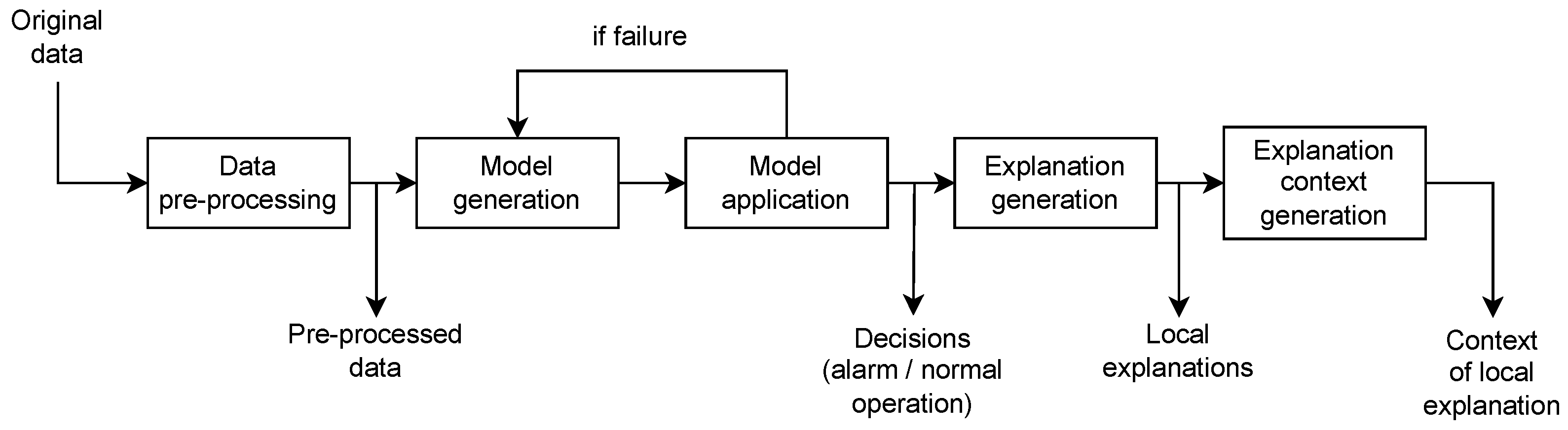
A general illustration of the process implemented within the experiments is presented in the diagram in Figure 1. This diagram depicts operations performed on data and their results. The first step of the process is pre-processing of the measurements creating original data set. Next, the model based on outlier identification is generated and applied to the data analysis. This model is re-generated following the annotation of machine failure in the data. For each recommendation provided by the model, a local explanation is generated. Finally, for each explanation, its context is presented. A more detailed description of the process elements is provided in the subsequent sections. The data set and its processing are described in Section 4.1. The selected methods generating the model and local explanations, and their experimental settings are presented in Section 4.2. The results containing local explanations and their context are presented in Section 4.3. Finally, the additional conclusions from the experiments are discussed in Section 4.4.
4.1. Data Set
The data set used in the experiments is based on the data reported in [11]. The initial data set consists of the measurements recorded for a coal crusher operating at the boiler of the power plant. The crusher, named NW-10, was equipped with two sensors C122 and C123 located on the opposite sides of the rotating shaft. The data collected by the sensors include three attributes: maximum and root mean square (RMS) value of vibration, and temperature. The measurement values were recorded every 10 s between 13 July 2019 and 30 March 2021. During this period, two machine failures requiring servicing operations were reported.
For the purpose of the analysis, the measurement values were aggregated within a time window of 8 h, which corresponds to the length of the shift. The aggregation resulted in a data set consisting of 717 examples that covered the period from the beginning of the measurements until the second machine failure. Two distinct approaches to aggregation were applied, which resulted in two different data representations. The first representation, hereinafter referred to as Basic, was calculated as a mean value of each attribute value within the time window. Therefore, Basic representation consists of six attributes, which correspond to the three measurements recorded by each of the two sensors (C122 and C123). The second representation, hereinafter referred to as Extended, was calculated by means of the tsfresh [36] library. This Python package offers methods for calculating a large number of time series characteristics. For each attribute of the data set, the following 15 statistical and time-based characteristics were calculated and taken as derived attributes: sum, median, mean, standard deviation, variance, root mean square, maximum, absolute maximum, minimum, intercept of the regression line, slope of the regression line, standard error of the estimated slope (gradient), assuming normality of the residuum, R value of the regression line, non-directional p-value for a test whose null hypothesis is that the slope is zero, using the Wald test with t distribution of the test statistic. Thus, the Extended representation consists of 90 attributes.
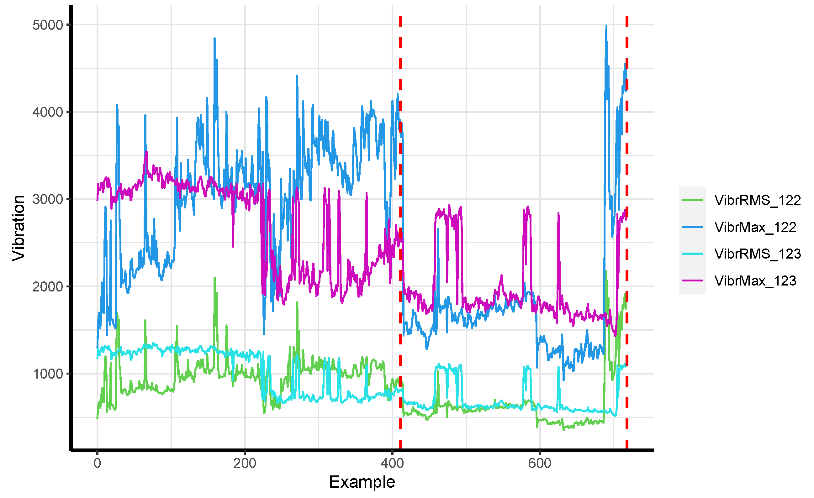
Figure 2 presents the values of the vibration-based attributes calculated for the Basic representation. In addition to the data characteristics, the figure presents when the failures took place in the form of dashed vertical lines. Looking at Figure 1, it can be noticed that around example 220 the characteristics of the measurements recorded by sensor C123 changed. Specifically, the values of VibrRMS_123 and VibrMax_123 decreased noticeably. This change occurs more than two months prior to Failure 1 and it can be interpreted as an indication of an impending failure, in a post hoc analysis. Similarly, it can be noticed that around example 600 the characteristics of the measurements recorded by sensor C122 changed. Specifically, the values of VibrRMS_122 and VibrMax_122 decreased noticeably. This change occurs almost one-and-a-half months prior to Failure 2 and it can be interpreted as an indication of an impending failure, in a post hoc analysis.
4.2. Experimental Settings
In this study, it was assumed that, due to the insufficient number of failure examples, the identification of the machine’s fault condition would be performed using an outlier identification algorithm. Following the approach validated in [11], the outlier identification method based on the HDBSCAN algorithm [37] and implemented in the hdbscan (https://hdbscan.readthedocs.io/en/latest) (accessed on 1 August 2023) Python library was chosen. HDBSCAN is a hierarchical density-based clustering algorithm that can be used to identify anomalies [38] by determining how much each data instance stands out. The initial 30 days of measurements were used as the initialisation period for the method. During this period the monitored machine was assumed to operate under normal conditions. After this period, the model was used to identify measurements that were anomalies, potentially indicating an impending failure. The model was used statically, with no adaptation of model parameters, until the failure occurred. After the failure, the model was generated again on data collected up to a week before the failure. The only parameter set for the HDBSCAN algorithm was min_cluster_size. The value of this parameter was assumed to be 0.01, as the share of outliers in the monitored data was assumed to be 1%.
For the purpose of generating explanations, the SHAP method [21] was selected. This well-established and frequently used method aligns with the assumptions set forth in this study. It generates local explanations in the form of an attribute ranking that illustrates attribute importance in the model’s decision-making. In this way, a user who needs to decide whether a reported alarm is indicating an impending failure can refer to the sensors (and their locations) represented by individual attributes. The generation of model decision explanations was performed in the shap (https://shap.readthedocs.io/en/latest/index.html) (accessed on 1 August 2023) Python library.
4.3. Results
4.3.1. Basic Representation
The first part of experiments was performed on the Basic data representation. To verify the quality of the created model, the number of outliers identified in the weeks following model training and preceding machine failure was calculated. The results are presented in Table 1. Common intuition suggests that at the very beginning (just after model training), a relatively small number of outliers should be identified. Whereas, in the period of time preceding a failure the number of identified outliers should be relatively high. The values in Table 1 reflect this intuition only for Failure 1. In case of Failure 2 the number of identified outliers is high from the very beginning. It suggests that the model is not well fitted to the distribution of data registered after Failure 1. Therefore, inferring an impending failure based on the increasing number of reported alarms would be possible for the generated model only before Failure 1.
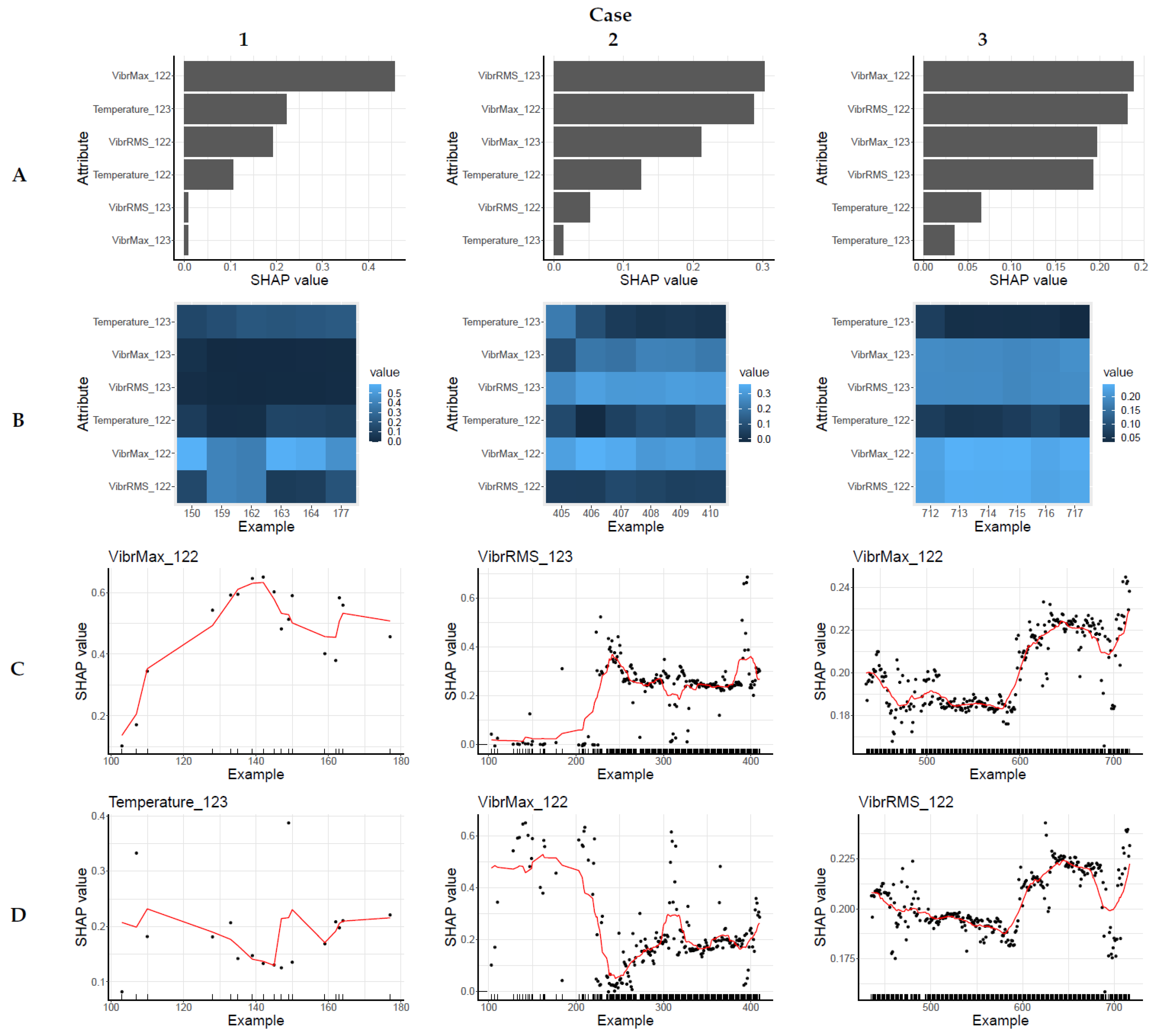
The explanations of selected decisions of the model trained on the Basic data representation are presented in Figure 3. Among the alarms identified by the model, a selection of three cases is presented in Figure 3. Case 1 is an alarm that was reported when the machine was operating correctly, i.e., relatively recently after the model was trained. With insights into the analysed data, it was assumed that an outlier identified after approximately four weeks was reported during correct machine operation. Thus, Case 1 presents example 87 (considering an 8 h aggregation window, 4 weeks corresponds to 84 examples). This instance was identified as the first outlier after four weeks, and the 17th outlier overall. Case 2 presents the last alarm before Failure 1, and Case 3 presents the last alarm before Failure 2.
An explanation of each alarm in Figure 3 consists of four figures (Figure 3A–D). Figure 3A presents a SHAP-based ranking of attribute importance. This is a typical local explanation. It identifies the attributes that have the greatest impact on the model’s decision. Figure 3B presents a local context to the SHAP-based explanation presented in Figure 3A. It has the form of a heatmap depicting attribute importance values for the alarm being explained and for the five preceding alarms. This figure (Figure 3B) allows for an assessment of how consistent the explanations for a given data instance are in comparison to those of examples that occurred at a similar time. It is of particular importance if the model based on outlier identification is used, as it visualises whether a class labelled as alarm has consistent explanations at a given time. In addition, this figure may help to identify an outlier among the outliers if a particular instance deviates significantly from the alarms immediately preceding it. Finally, Figure 3C,D present the global contexts to the SHAP-based explanation presented in Figure 3A. The global context is generated for each attribute independently. Figure 3 presents the global context for the most important attribute (C) according to the SHAP-based explanation and the second most important attribute (D). The figures presenting global context contain a scatter plot of all the attribute importance values calculated for the preceding examples of the alarm class. Moreover, there is a line in the figure representing the smoothed mean of the plotted values to support interpretation of the data characteristics. The mean value for the example was determined as follows:
where , , n is the number of data examples forming the context and visualisation, is a smoothing window size, and is a parameter defining the size of the smoothing window and it was set to 0.1. Additionally, each scatter plot has a rug plot on the x axis illustrating the density of the identified alarms.
The basic results presented in Figure 3 are the SHAP-based explanations consisting of the attribute rankings presented in Figure 3A. Case 1 represents the outlier identified during the correct machine operation; therefore, for Case 1, Figure 3A does not allow any conclusions to be drawn with regard to supporting the identification of the pre-failure state of the machine. The analyses of the next two cases can be performed regarding data characteristics presented in Section 4.1. They showed that the values measured by sensor C123 may carry important information about the impending Failure 1 and the values measured by sensor C122 may carry important information about the impending Failure 2. The explanation of Case 2 presented in Figure 3A shows that vibrations measured by sensor C123 were among the most important for the decision of the model, whereas the explanation of Case 3 presented in Figure 3A shows that vibrations measured by sensor C122 were the most important. Thus, the SHAP-based explanations are consistent with conclusions based on the distribution of data and can support decision-making.
The local context (Figure 3B) shown for each explanation is consistent, i.e., the attribute importance rankings are similar for the alarms reported most recently. This means that the alarm class definition is consistent for the recent examples.
The results show that the global context presented in Figure 3C,D for the most significant attributes provides valuable additional information. For Case 1, this context consists of relatively few examples and the plot they create does not illustrate any clear trend. For Case 2 and Case 3, the context in Figure 3C,D shows a clear change in SHAP-determined attribute importance. This change means that the characteristics of the class whose examples were identified have changed. Assuming that the machine was working correctly at the beginning, a change in the concept alarm may indicate an impending failure. Moreover, the changes in characteristics visible in Figure 3C,D in Cases 2 and 3 are consistent with the change in characteristics of the recorded measurements presented in Section 4.1.
Furthermore, in Case 2, with the change in attribute importance, the density of identified alarms increased. An increase in alarms reported should be regarded as a clear indicator of impending failure. The alarm frequency for the global context for Case 1 is relatively low, which is consistent with the fact that this period is unrelated to the failure. In contrast, in Case 3 the frequency of reported alarms is very high from the very beginning, indicating a poorly calibrated model that identifies too many outliers.
4.3.2. Extended Representation
For the Extended data representation, similar analyses to those presented above were performed. Table 2 presents the number of outliers identified in the weeks following model training and preceding machine failure. The model based on the Extended data representation did not improve the distinction between the period of normal machine operation and the period prior to the machine failure. In the case of Failure 1, the number of alarms is only slightly lower during normal operation, and there are no significant differences between the two periods in the case of Failure 2.
The Extended representation contains many attributes that are hardly informative to the machine operator. Consequently, additional processing is required to derive explanations of the model decisions that are understandable to the user. Therefore, the explanations generated by SHAP as the importance value of the derived attributes were aggregated to the basic attributes associated with the recorded measurements. Different aggregation functions were applied and evaluated. To select the best method of aggregation, the SHAP rankings determined for the Basic representation were chosen as a reference point. Table 3 presents Pearson correlation and root mean square error (RMSE) values assessing the similarity of the SHAP rankings for the two representations. The worst of the methods compared in Table 3 was Median, while the most stable quality results were obtained for Max. Among the best results obtained were those generated for the Sum function and this aggregation function was used in further analyses.
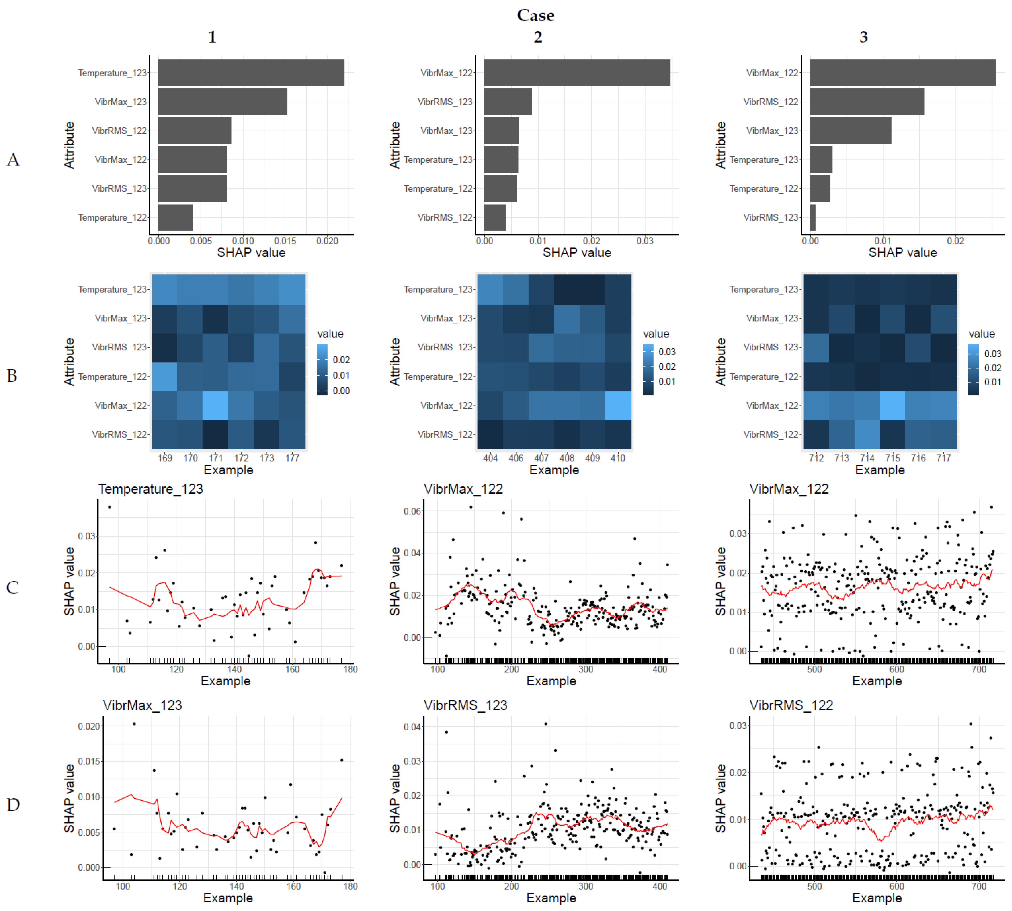
The explanations for selected decisions of the model trained on the Extended data representation are presented in Figure 4. The analysis procedure mirrors that of the Basic representation (Figure 3). Therefore, a selection of three cases is presented in Figure 4. Case 1 is an alarm reported when the machine was operating correctly, i.e., relatively recently after the model was trained (approximately four weeks). For Extended representation, Case 1 refers to example 87, which was identified as the first outlier after four weeks, and the 48th outlier overall. Case 2 presents the last alarm before Failure 1, and Case 3 presents the last alarm before Failure 2.
The SHAP-based explanations of the true alarms (Case 2 and 3) presented in Figure 4 A are not perfectly correlated with the conclusions drawn from the analysis of the measurement characteristics. For Case 2, the attribute associated with the C122 sensor is the most important. The attributes associated with the C123 sensor (which, based on measurement characteristics, seemed to be important before Failure 1) are ranked next but their importance is significantly lower. In Case 3, as expected, the attributes associated with the vibration measurements from the C122 sensor are the most important.
The local context of the SHAP-based explanations is presented in Figure 4B. Although Case 1 presents false alarms, it contains one stable indication that temperature measured by the C123 sensor was important for all decisions considered for this case. In Case 2, the explanations forming the local context differ to such an extent that it is easier to identify what was not important (temperature and RMS of vibration measured by the C122 sensor), than what was important for the presented group of decisions. In Case 3, the local context shows that vibration measurements from the C122 sensor were the most important for this group of model decisions.
The global context of the SHAP-based explanations is presented in Figure 4C,D. In Case 1, it is not possible to discern clear trends or long-term changes in the importance of the most important attributes. In Case 2 such changes can be identified; however, they are not very clear. In Case 3, long-term changes in the value distributions do not occur, even though the analysis of the measurements (Section 4.1) suggests that they should be visible.
4.4. Discussion
A comparison of the proposed explanation context for the Basic and Extended data representations, which are presented in Figure 3 and Figure 4, shows considerable differences. The local context of the SHAP-based explanations for the Extended data representation (Figure 4B) is significantly less cohesive for each of the Cases compared to the results from the Basic data representation (Figure 3B). The attribute importance values, and the attribute ranking, fluctuate significantly and fail to form a consistent description indicating which attributes are important for the decision on the alarm class. Moreover, the global context of the SHAP-based explanations presented in Figure 4C,D is significantly less informative when comparing to the results of the Basic data representation presented in Figure 3C,D. The attribute importance values presented on the plots do not show clear (or any) long-term changes. Therefore, the figures do not support conclusions about the current machine state.
This implies that the proposed explanation context, designed to support the operator’s understanding of the machine state, is significantly less helpful for the model based on Extended data representation, despite the application of explanation aggregation. Addressing this challenge could involve the use of an explanation by simplification approach, employing a surrogate model. In the case of the analysed task, the surrogate model is the model generated from the Basic data representation. Therefore, generating a local explanation for the alarm decision of the model based on Extended data representation should consist of the following steps:
- Verification if the similar alarm was generated by the surrogate model on the Basic data representation;
- If yes, generation of a local explanation and its context for the decision of the surrogate model;
- Otherwise, generation of an aggregated local explanation for the decision of the model based on the Extended data representation and visualisation of the context for the recent alarm decision of surrogate model.
This approach is reasonable because most of the alarms identified for the Extended data representation were identified as alarms for the Basic representation. Considering the time period until Failure 1, during which alarms were less frequent, almost 73% of outliers identified in the Extended data representation were identified in the Basic representation. If a surrogate model is used for the analysed data set, all alarms for which explanations are given in Figure 4 will receive explanations from Figure 3. This will significantly improve the comprehensibility of the model’s decisions.
5. Conclusions
This paper proposes to extend the typical local explanations presenting attribute importance with an illustration of the context for these explanations. The research is motivated by the need to better explain the decisions of a model identifying outliers in temporal data. These models are often used in predictive maintenance tasks and a real-world industrial application was the starting point for this study. The proposed XAI solutions aim to support machine operator decision-making and they were verified on real industrial data.
When utilising outlier detection to determine the state of a machine, it is not clear whether an alarm is an anomaly or an example of an alarm class indicating an impending failure. A better understanding of this issue is provided by the proposed two types of explanation contexts: local and global. The determination of these contexts is possible due to the temporal nature of the analysed data.
The analysis of the experimental results has shown that the typical local explanations generated by the SHAP method do not provide sufficient information needed to understand the model’s decision concerning the current state of the machine. However, the presented results demonstrate that extending the explanations to include local context supports verification whether recently reported alarms had consistent characteristics. In addition, the global context supports identification of changes in the attribute importance distribution. These changes may indicate a modification in class definition due to the deteriorating condition of the monitored machine. Thus, the proposed contexts can provide validation to the reported alarms.
Furthermore, the experimental results show that the use of a model based on data with numerous derived attributes significantly weakens the clarity of explanations and their contexts. The proposed solution to this problem is explanation by simplification, involving the use of explanations and their context generated for the decisions of a surrogate model created for the basic attributes.
Future works foreseen for this subject include validation of the proposed approach for other XAI methods, e.g., RuleXAI [23], where explanations can be more detailed yet are potentially more difficult to use when determining context. Furthermore, it will be important to automate inference based on the proposed explanation context to simplify support for the machine operator.
Funding
This research was funded by Computer Networks and Systems Department at Silesian University of Technology within the statutory research project.
Institutional Review Board Statement
Not applicable.
Informed Consent Statement
Not applicable.
Data Availability Statement
The SHAP-based explanation data set presented and analysed in this study is openly available in: http://adaa.polsl.pl/index.php/datasets-software/ accessed on: 4 September 2023.
Acknowledgments
Acknowledgments to Bartosz Piguła for his technical support.
Conflicts of Interest
The authors declare no conflict of interest. The funders had no role in the design of the study; in the collection, analyses, or interpretation of data; in the writing of the manuscript; or in the decision to publish the results.
References
- Gunning, D. Explainable Artificial Intelligence (XAI); nd Web; Defense Advanced Research Projects Agency (DARPA): Arlington, VA, USA, 2017; Volume 2, p. 1. [Google Scholar]
- Goodman, B.; Flaxman, S. European Union Regulations on Algorithmic Decision-Making and a “Right to Explanation”. AI Mag. 2017, 38, 50–57. [Google Scholar] [CrossRef]
- Tjoa, E.; Guan, C. A Survey on Explainable Artificial Intelligence (XAI): Toward Medical XAI. IEEE Trans. Neural Netw. Learn. Syst. 2021, 32, 4793–4813. [Google Scholar] [CrossRef] [PubMed]
- Antoniadi, A.M.; Du, Y.; Guendouz, Y.; Wei, L.; Mazo, C.; Becker, B.A.; Mooney, C. Current Challenges and Future Opportunities for XAI in Machine Learning-Based Clinical Decision Support Systems: A Systematic Review. Appl. Sci. 2021, 11, 5088. [Google Scholar] [CrossRef]
- Martino, F.D.; Delmastro, F. Explainable AI for clinical and remote health applications: A survey on tabular and time series data. Artif. Intell. Rev. 2022, 56, 5261–5315. [Google Scholar] [CrossRef]
- Sachan, S.; Yang, J.B.; Xu, D.L.; Benavides, D.E.; Li, Y. An explainable AI decision-support-system to automate loan underwriting. Expert Syst. Appl. 2020, 144, 113100. [Google Scholar] [CrossRef]
- Vollert, S.; Atzmueller, M.; Theissler, A. Interpretable Machine Learning: A brief survey from the predictive maintenance perspective. In Proceedings of the 2021 26th IEEE International Conference on Emerging Technologies and Factory Automation (ETFA ), Vasteras, Sweden, 7–10 September 2021; pp. 1–8. [Google Scholar] [CrossRef]
- Pashami, S.; Nowaczyk, S.; Fan, Y.; Jakubowski, J.; Paiva, N.; Davari, N.; Bobek, S.; Jamshidi, S.; Sarmadi, H.; Alabdallah, A.; et al. Explainable Predictive Maintenance. arXiv 2023, arXiv:2306.05120. [Google Scholar]
- Biecek, P.; Burzykowski, T. Explanatory Model Analysis: Explore, Explain and Examine Predictive Models; Chapman and Hall/CRC: Boca Raton, FL, USA, 2021. [Google Scholar]
- Molnar, C. Interpretable Machine Learning, 2nd ed.; 2022; Available online: https://leanpub.com/ (accessed on 4 September 2023).
- Hermansa, M.; Kozielski, M.; Michalak, M.; Szczyrba, K.; Wróbel, L.; Sikora, M. Sensor-Based Predictive Maintenance with Reduction of False Alarms—A Case Study in Heavy Industry. Sensors 2021, 22, 226. [Google Scholar] [CrossRef] [PubMed]
- Adadi, A.; Berrada, M. Peeking Inside the Black-Box: A Survey on Explainable Artificial Intelligence (XAI). IEEE Access 2018, 6, 52138–52160. [Google Scholar] [CrossRef]
- Barredo Arrieta, A.; Díaz-Rodríguez, N.; Del Ser, J.; Bennetot, A.; Tabik, S.; Barbado, A.; Garcia, S.; Gil-Lopez, S.; Molina, D.; Benjamins, R.; et al. Explainable Artificial Intelligence (XAI): Concepts, taxonomies, opportunities and challenges toward responsible AI. Inf. Fusion 2020, 58, 82–115. [Google Scholar] [CrossRef]
- Došilović, F.K.; Brčić, M.; Hlupić, N. Explainable artificial intelligence: A survey. In Proceedings of the 2018 41st International Convention on Information and Communication Technology, Electronics and Microelectronics (MIPRO), Opatija, Croatia, 21–25 May 2018; pp. 210–215. [Google Scholar]
- Guidotti, R.; Monreale, A.; Ruggieri, S.; Turini, F.; Giannotti, F.; Pedreschi, D. A Survey of Methods for Explaining Black Box Models. ACM Comput. Surv. 2018, 51, 1–42. [Google Scholar] [CrossRef]
- Holzinger, A.; Saranti, A.; Molnar, C.; Biecek, P.; Samek, W. Explainable AI Methods—A Brief Overview. In xxAI—Beyond Explainable AI: International Workshop, Held in Conjunction with ICML 2020, 18 July 2020, Vienna, Austria, Revised and Extended Papers; Springer International Publishing: Cham, Switzerland, 2022; pp. 13–38. [Google Scholar] [CrossRef]
- Linardatos, P.; Papastefanopoulos, V.; Kotsiantis, S. Explainable AI: A Review of Machine Learning Interpretability Methods. Entropy 2020, 23, 18. [Google Scholar] [CrossRef] [PubMed]
- Mohseni, S.; Zarei, N.; Ragan, E.D. A Multidisciplinary Survey and Framework for Design and Evaluation of Explainable AI Systems. ACM Trans. Interact. Intell. Syst. 2021, 11, 1–45. [Google Scholar] [CrossRef]
- Guidotti, R. Counterfactual explanations and how to find them: Literature review and benchmarking. Data Min. Knowl. Discov. 2022, 2022, 1–55. [Google Scholar] [CrossRef]
- Goldstein, A.; Kapelner, A.; Bleich, J.; Pitkin, E. Peeking Inside the Black Box: Visualizing Statistical Learning With Plots of Individual Conditional Expectation. J. Comput. Graph. Stat. 2015, 24, 44–65. [Google Scholar] [CrossRef]
- Lundberg, S.M.; Lee, S.I. A Unified Approach to Interpreting Model Predictions. In Proceedings of the Advances in Neural Information Processing Systems; Guyon, I., Luxburg, U.V., Bengio, S., Wallach, H., Fergus, R., Vishwanathan, S., Garnett, R., Eds.; Curran Associates, Inc.: Red Hook, NY, USA, 2017; Volume 30. [Google Scholar]
- Ribeiro, M.; Singh, S.; Guestrin, C. “Why Should I Trust You?”: Explaining the Predictions of Any Classifier. In Proceedings of the 2016 Conference of the North American Chapter of the Association for Computational Linguistics: Demonstrations, San Diego, CA, USA, 12–17 June 2016; pp. 97–101. [Google Scholar] [CrossRef]
- Macha, D.; Kozielski, M.; Wróbel, L.; Sikora, M. RuleXAI—A package for rule-based explanations of machine learning model. SoftwareX 2022, 20, 101209. [Google Scholar] [CrossRef]
- Tripathy, S.M.; Chouhan, A.; Dix, M.; Kotriwala, A.; Klöpper, B.; Prabhune, A. Explaining Anomalies in Industrial Multivariate Time-series Data with the help of eXplainable AI. In Proceedings of the 2022 IEEE International Conference on Big Data and Smart Computing (BigComp), Daegu, Korea, 17–20 January 2022; pp. 226–233. [Google Scholar] [CrossRef]
- Rojat, T.; Puget, R.; Filliat, D.; Del Ser, J.; Gelin, R.; Díaz-Rodríguez, N. Explainable Artificial Intelligence (XAI) on TimeSeries Data: A Survey. arXiv 2021, arXiv:2104.00950. [Google Scholar]
- Lin, J.; Keogh, E.; Wei, L.; Lonardi, S. Experiencing SAX: A novel symbolic representation of time series. Data Min. Knowl. Discov. 2007, 15, 107–144. [Google Scholar] [CrossRef]
- Ye, L.; Keogh, E. Time series shapelets: A novel technique that allows accurate, interpretable and fast classification. Data Min. Knowl. Discov. 2010, 22, 149–182. [Google Scholar] [CrossRef]
- Abanda, A.; Mori, U.; Lozano, J. Ad-hoc explanation for time series classification. Knowl.-Based Syst. 2022, 252, 109366. [Google Scholar] [CrossRef]
- Schoonderwoerd, T.A.; Jorritsma, W.; Neerincx, M.A.; van den Bosch, K. Human-centered XAI: Developing design patterns for explanations of clinical decision support systems. Int. J. Hum.-Comput. Stud. 2021, 154, 102684. [Google Scholar] [CrossRef]
- Serradilla, O.; Zugasti, E.; Ramirez de Okariz, J.; Rodriguez, J.; Zurutuza, U. Adaptable and Explainable Predictive Maintenance: Semi-Supervised Deep Learning for Anomaly Detection and Diagnosis in Press Machine Data. Appl. Sci. 2021, 11, 7376. [Google Scholar] [CrossRef]
- Jakubowski, J.; Stanisz, P.; Bobek, S.; Nalepa, G.J. Explainable anomaly detection for Hot-rolling industrial process. In Proceedings of the 2021 IEEE 8th International Conference on Data Science and Advanced Analytics (DSAA), Porto, Portugal, 6–9 October 2021; pp. 1–10. [Google Scholar] [CrossRef]
- Jakubowski, J.; Stanisz, P.; Bobek, S.; Nalepa, G.J. Anomaly Detection in Asset Degradation Process Using Variational Autoencoder and Explanations. Sensors 2022, 22, 291. [Google Scholar] [CrossRef] [PubMed]
- Jakubowski, J.; Stanisz, P.; Bobek, S.; Nalepa, G.J. Roll Wear Prediction in Strip Cold Rolling with Physics-Informed Autoencoder and Counterfactual Explanations. In Proceedings of the 2022 IEEE 9th International Conference on Data Science and Advanced Analytics (DSAA), Shenzhen, China, 13–16 October 2022; pp. 1–10. [Google Scholar] [CrossRef]
- Randriarison, J.J.; Rajaoarisoa, L.; Sayed-Mouchaweh, M. Faults explanation based on a machine learning model for predictive maintenance purposes. In Proceedings of the 2023 International Conference on Control, Automation and Diagnosis (ICCAD), Rome, Italy, 10–12 May 2023; pp. 1–6. [Google Scholar] [CrossRef]
- Sayed-Mouchaweh, M.; Rajaoarisoa, L. Explainable Decision Support Tool for IoT Predictive Maintenance within the context of Industry 4.0. In Proceedings of the 2022 21st IEEE International Conference on Machine Learning and Applications (ICMLA), Nassau, Bahamas, 12–14 December 2022; pp. 1492–1497. [Google Scholar] [CrossRef]
- Christ, M.; Braun, N.; Neuffer, J.; Kempa-Liehr, A.W. Time Series FeatuRe Extraction on Basis of Scalable Hypothesis Tests (Tsfresh—A Python Package). Neurocomputing 2018, 307, 72–77. [Google Scholar] [CrossRef]
- Campello, R.J.G.B.; Moulavi, D.; Sander, J. Density-Based Clustering Based on Hierarchical Density Estimates. In Advances in Knowledge Discovery and Data Mining; Hutchison, D., Kanade, T., Kittler, J., Kleinberg, J.M., Mattern, F., Mitchell, J.C., Naor, M., Nierstrasz, O., Pandu Rangan, C., Steffen, B., et al., Eds.; Springer: Berlin/Heidelberg, Germnay, 2013; Volume 7819, pp. 160–172. [Google Scholar] [CrossRef]
- Campello, R.J.G.B.; Moulavi, D.; Zimek, A.; Sander, J. Hierarchical Density Estimates for Data Clustering, Visualization, and Outlier Detection. ACM Trans. Knowl. Discov. Data 2015, 10, 1–51. [Google Scholar] [CrossRef]
Figure 1.
Diagram of the process implemented in the experiments.

Figure 2.
Values of the selected attributes (representing vibrations [mg]) of crusher data set, machine failures are marked by red dashed vertical lines.
Figure 2.
Values of the selected attributes (representing vibrations [mg]) of crusher data set, machine failures are marked by red dashed vertical lines.

Figure 3.
Selected SHAP-based explanations of the model decisions and their contexts for Basic data representation—the selected data instances contain the following: alarm from the period of normal machine operation (Case 1), last alarm before Failure 1 (Case 2), last alarm before Failure 2 (Case 3). The figures present SHAP-based attribute importance ranking (A), local context heatmap (B), global context for the most important attribute indicated by SHAP (C), global context for the second most important attribute indicated by SHAP (D).

Figure 4.
Selected SHAP-based explanations of the model decisions and their contexts for Extended data representation and Sum aggregation—the selected data instances contain the following: alarm from the period of the normal machine operation (Case 1), last alarm before Failure 1 (Case 2), last alarm before Failure 2 (Case 3). The figures present local explanations, where attribute importances were aggregated using the sum operation: SHAP-based attribute importance ranking (A), local context heatmap (B), global context for the most important attribute indicated by SHAP (C), global context for the second most important attribute indicated by SHAP (D).


Table 1.
Number of alarms (outliers) identified in data (Basic representation) collected before Failure 1 and afterwards until Failure 2; Ti represents week number after model training (when the machine is operating correctly), Fi represents week number before failure.
Table 1.
Number of alarms (outliers) identified in data (Basic representation) collected before Failure 1 and afterwards until Failure 2; Ti represents week number after model training (when the machine is operating correctly), Fi represents week number before failure.
| T1 | T2 | T3 | F3 | F2 | F1 | |
|---|---|---|---|---|---|---|
| Failure 1 | 3 | 1 | 8 | 21 | 21 | 21 |
| Failure 2 | 21 | 19 | 15 | 21 | 19 | 21 |
Table 2.
Number of alarms (outliers) identified in data (Extended representation) collected before Failure 1 and afterwards until Failure 2; Ti represents week number after model training (when the machine is operating correctly), Fi represents week number before failure.
Table 2.
Number of alarms (outliers) identified in data (Extended representation) collected before Failure 1 and afterwards until Failure 2; Ti represents week number after model training (when the machine is operating correctly), Fi represents week number before failure.
| T1 | T2 | T3 | F3 | F2 | F1 | |
|---|---|---|---|---|---|---|
| Failure 1 | 4 | 13 | 17 | 19 | 20 | 17 |
| Failure 2 | 21 | 20 | 20 | 21 | 21 | 21 |
Table 3.
Evaluation of similarity between attribute importance rankings determined for Basic and Extended data representations.
Table 3.
Evaluation of similarity between attribute importance rankings determined for Basic and Extended data representations.
| Correlation | RMSE | |||||||
|---|---|---|---|---|---|---|---|---|
| Sum | Max | Mean | Median | Sum | Max | Mean | Median | |
| Failure 1 | 0.22 | 0.54 | 0.22 | −0.05 | 8.50 | 7.11 | 8.51 | 9.29 |
| Failure 2 | 0.87 | 0.48 | 0.87 | 0.06 | 2.92 | 7.28 | 2.91 | 8.27 |
Disclaimer/Publisher’s Note: The statements, opinions and data contained in all publications are solely those of the individual author(s) and contributor(s) and not of MDPI and/or the editor(s). MDPI and/or the editor(s) disclaim responsibility for any injury to people or property resulting from any ideas, methods, instructions or products referred to in the content. |
© 2023 by the author. Licensee MDPI, Basel, Switzerland. This article is an open access article distributed under the terms and conditions of the Creative Commons Attribution (CC BY) license (https://creativecommons.org/licenses/by/4.0/).
Share and Cite
MDPI and ACS Style
Kozielski, M. Contextual Explanations for Decision Support in Predictive Maintenance. Appl. Sci. 2023, 13, 10068. https://doi.org/10.3390/app131810068
AMA Style
Kozielski M. Contextual Explanations for Decision Support in Predictive Maintenance. Applied Sciences. 2023; 13(18):10068. https://doi.org/10.3390/app131810068
Chicago/Turabian StyleKozielski, Michał. 2023. "Contextual Explanations for Decision Support in Predictive Maintenance" Applied Sciences 13, no. 18: 10068. https://doi.org/10.3390/app131810068
Note that from the first issue of 2016, this journal uses article numbers instead of page numbers. See further details here.