Detecting and Isolating Adversarial Attacks Using Characteristics of the Surrogate Model Framework

Abstract

The paper introduces a novel framework for detecting adversarial attacks on machine learning models that classify tabular data. Its purpose is to provide a robust method for the monitoring and continuous auditing of machine learning models for the purpose of detecting malicious data alterations. The core of the framework is based on building machine learning classifiers for the detection of attacks and its type that operate on diagnostic attributes. These diagnostic attributes are obtained not from the original model, but from the surrogate model that has been created by observation of the original model inputs and outputs. The paper presents building blocks for the framework and tests its power for the detection and isolation of attacks in selected scenarios utilizing known attacks and public machine learning data sets. The obtained results pave the road for further experiments and the goal of developing classifiers that can be integrated into real-world scenarios, bolstering the robustness of machine learning applications.

1. Introduction

The rise of widespread usage of machine learning (ML) has changed many areas of our lives by allowing the automation of processes based on real-time analysis of vast amounts of data [1]. But, as the use of ML grows, so do concerns about its safety and trustworthiness. Historically, the approach to trustworthy AI has been characterized by efforts to promote transparency and interpretability of ML models, which involve understanding the decision-making processes of ML models, enabling humans to comprehend and trust their outputs [2]. Concurrently, studies have underscored the importance of robustness against adversarial attacks (AA) on ML models. In these scenarios, malevolent actors introduce intentional perturbations, aimed at causing unintended behavior of ML models [3,4]. As a response to these threats, a whole new field of adversarial attack detection and prevention has arisen [5,6,7].

Work Motivation

The motivation for our work is to verify the practical usefulness of a new method for detecting adversarial attacks on ML models, thus increasing the robustness of ML applications. The specific method used came from the realization that:

• There are no well-established AA detection methods that attempt to analyze machine learning models during their operations that can work in a black-box scenario.
• Rough sets theory–based methods [8,9] can be used to approximate the decision boundaries of a classifier model, thus allowing for the reconstruction of a model with no direct access, creating a surrogate model that can be then analyzed with full access to it.
• Most AA detection techniques focus on image processing models [10], with tabular data techniques receiving attention only in recent years [11].

Our end goal is to create a robust framework that can be used in real-world applications for the continuous monitoring of machine learning models, thus increasing the safety and trustworthiness of machine learning applications in everyday scenarios.

Within this work, we assume a black-box scenario, which we define as a lack of access to internal knowledge of the machine learning model operations, neither its architecture nor its internal states. Instead, interested parties can only observe the inputs and outputs of machine learning model operations and need to drive their conclusions on the machine learning model characteristics from these observations. While this scenario is often assumed for the attacking party, defense mechanisms often assume full knowledge of the observed model, which is not true in many real-world scenarios.

2. Related Work

2.1. Adversarial Attacks

Since the beginning of the adversarial machine learning (AML) research field [12,13], many attempts have been made to create taxonomies of attacks [10,14]. On the basic plane, adversarial machine learning attacks can be categorized broadly into several types based on various criteria such as the attacker’s knowledge, the attacker’s capabilities, and the attack’s target.

The most commonly used types include the following. (1) White-Box vs. Black-Box Attacks: In a white-box attack, the adversary has complete knowledge of the model, including its architecture and parameters. This allows for the creation of sophisticated and highly effective adversarial examples. In contrast, a black-box attack assumes limited knowledge of the model, with the adversary potentially only having access to input-output pairs. The transferability of adversarial examples is often exploited in black-box attacks [4]. (2) Evasion vs. Poisoning Attacks: Evasion attacks occur at the test phase where adversarial examples are crafted to mislead the model’s prediction. This is often achieved by adding carefully designed noise to the input [13]. In poisoning attacks, the training phase is targeted where the adversary manipulates the training data to compromise the learning process itself, leading to incorrect models being learned [15].

(3) Targeted vs. Non-Targeted Attacks: In a targeted attack, the goal of the adversary is to cause a specific misclassification, e.g., making a model classify a stop sign as a speed limit sign. Non-targeted attacks aim to cause any misclassification, without a specific target in mind [5]. (4) Exploratory vs. Causative Attacks: This classification overlaps somehow with the Evasion vs. Poisoning dichotomy, but it was historically the first classification type. In exploratory attacks, the adversary exploits a model’s weaknesses after being trained. In contrast, causative attacks involve influencing the learning process to introduce specific vulnerabilities that can be exploited later [16].

Each type of attack requires different detection and defense strategies, emphasizing the importance of understanding the specific adversarial landscape when building robust machine learning models. In this work, we focus on detecting exploratory (evasion) attacks in black-box scenarios, targeting models processing tabular data [17,18,19].

2.2. Adversarial Defenses

Defenses against adversarial attacks can be divided into two groups: detection and preventive methods.

The main detection methods reported in the literature include:

• Statistical Tests: These involve conducting statistical analyses on model inputs to identify irregularities or anomalies indicative of adversarial manipulation. For instance, a technique based on the L1-norm to detect adversarial attacks was proposed by Grosse et al. [20,21].
• Reconstruction-based Methods: These techniques rely on reconstructing the input and comparing it with the original input to identify adversarial perturbations. One approach is to use autoencoder-based methods for input reconstruction [22]. This technique can be part of a larger detection framework, such as [23].
• Feature Squeezing: This technique can be used both for the detection of adversarial examples and for increasing the innate robustness of machine learning models. Since it reduces the search space available to an adversary by compressing the amount of expressiveness in the input, it makes all adversarial modifications more apparent thanks to the simplification of model inputs [24].
• Classifier-based Methods: These approaches involve training a separate classifier to discern between adversarial and legitimate inputs, such as Metzen et al.’s method using a trained auxiliary neural network [21]. Another example is a MagNet framework, which consists of both detector and reformer networks. Detector networks are used to classify examples as either normal or adversarial, by approximating the manifold of normal examples. The reformer network is then used to move adversarial examples towards the manifold of normal examples—resulting in the correct classification of adversarial examples with small perturbation [23].

Another stream of work is related to creating methods of implementing innate robustness against adversarial machine learning attacks into machine learning models themselves.

These methods include:

• Adversarial Training: This technique aims to improve the model’s resilience against adversarial attacks by explicitly including adversarial examples in the training process. The underlying idea is to expose the model to these specially crafted deceptive inputs during training, forcing the model to learn from these examples and consequently enhancing its robustness. Goodfellow et al. proposed the concept in their pioneering work, thus adding a new dimension to the understanding of model generalization and resilience [12].
• Defensive Distillation: This technique involves training the model to provide softer output distributions rather than discrete class labels, thereby rendering the model’s decision boundaries smoother and less prone to adversarial perturbations. The distillation process increases the model’s resilience against adversarial attacks by reducing the effectiveness of small perturbations on the input. The technique was described in depth by Papernot et al. [25].
• Feature Squeezing: This technique aims to mitigate the risk of adversarial attacks by reducing the complexity of model inputs, effectively limiting the scope for adversarial manipulation. By squeezing or reducing the input data’s expressiveness, the technique narrows down the available search space that an adversary could exploit [24].
• Certified Defenses: These methods provide mathematical guarantees of a model’s robustness against adversarial attacks. Rather than solely relying on empirical assessments of model performance, these defenses offer a theoretical underpinning to ensure robustness, thus contributing to a more rigorous and reliable model defense. The core concept is to mathematically certify a region around each data point within which the model’s prediction remains consistent, hence making it robust against adversarial perturbations [26].

We strive to enhance this list by presenting a new method useful in black-box scenarios on tabular data.

3. Methods

In this section, we presented the workflow of the whole analysis, the definition of analyzed adversarial attacks, and the detection algorithm. Figure 1 shows a diagram with the overall analysis workflow.

We started by training the machine learning model and obtaining predictions for the new data set using this model. Based on provided data and the training data set, approximator learning is conducted, which ends with diagnostic attributes calculations. Simultaneously, an adversarial attack on the data can be executed, which results in obtaining perturbed data set with model predictions. Utilization of trained approximator model allows us to calculate diagnostic attributes for new (perturbed) incoming data. The application of this workflow for many data sources and different attacks results in the acquisition of such information (original diagnostic attributes and perturbed diagnostic attributes), which, after aggregation, are used for training models for the detection and isolation of adversarial attacks.

3.1. Attacks Detected

We have tested the method against three different types of adversarial attacks: HopSkipJump, PermuteAttack, and ZOO. These attacks have been chosen based on the following common characteristics:

• Academic renown of the original publication and subsequent publications exploring each specific attack;
• Suitability to operate on tabular data;
• Attempt to hide their operations—perturbances introduced are minimally required for a successful attack;
• Having an available implementation code base.

The HopSkipJump attack, also known as the Decision-Based Boundary attack, is an adversarial attack that manipulates both the local and global aspects of the decision boundary of the model under attack, thus causing misclassification while minimizing the perturbation on the original input [17].

It is an iterative, decision-based attack, meaning that it only requires access to the model’s output decisions (e.g., classification labels) rather than full access to the model’s internal workings or gradients; it can function in a black-box environment where access to the model specifics is limited.

The attack algorithm consists of three main steps:

• Initialization (Hop): A starting point for the adversarial example is identified, which lies on the opposite side of the decision boundary compared to the target input.
• Binary Search (Skip): A binary search strategy is implemented to bring the adversarial example closer to the decision boundary without crossing it.
• Gradient Estimation (Jump): By making small perturbations to the adversarial example and observing the model’s outputs, an approximation of the gradient at the decision boundary is estimated. This gradient information is then utilized to make a controlled jump that slightly crosses the decision boundary, making the adversarial example more effective.

The PermuteAttack, described in [18], is an adversarial example generation method capable of handling tabular data including discrete and categorical variables. The method utilizes a gradient-free optimization approach founded on genetic algorithms, which applies permutations to a random selection of features while ensuring the resultant values adhere to acceptable data set ranges. As a result, the output contains counterfactual data points that, though altered from the original data points, can circumvent certain anomaly detection methods. The resulting adversarial examples can serve as analytical tools for assessing the robustness of the attacked model.

The Zeroth Order Optimization (ZOO) adversarial attack, introduced in [19], is a black-box attack method that utilizes zeroth-order (derivative-free) optimization to construct adversarial examples. The ZOO attack is designed to be applicable even when the attacker only has access to the model’s output (like probabilities of classes) and does not know about the model’s architecture or parameters.

In the ZOO attack, the attacker starts with a legitimate sample and incrementally perturbs it by approximating the gradients of the loss function. These approximations are obtained through numerical methods such as finite difference methods, and they do not require access to the actual gradients of the loss function.

The attacker then uses the estimated gradients to iteratively modify the input, typically via a method similar to the Fast Gradient Sign Method (FGSM), a popular attack method in white-box settings. This process continues until the modified input misleads the model into making an incorrect prediction.

This attack method demonstrated that efficient and effective black-box attacks are possible, even without direct access to gradient information. As a result, it underscored the importance of considering black-box attack scenarios when developing defenses for machine learning models.

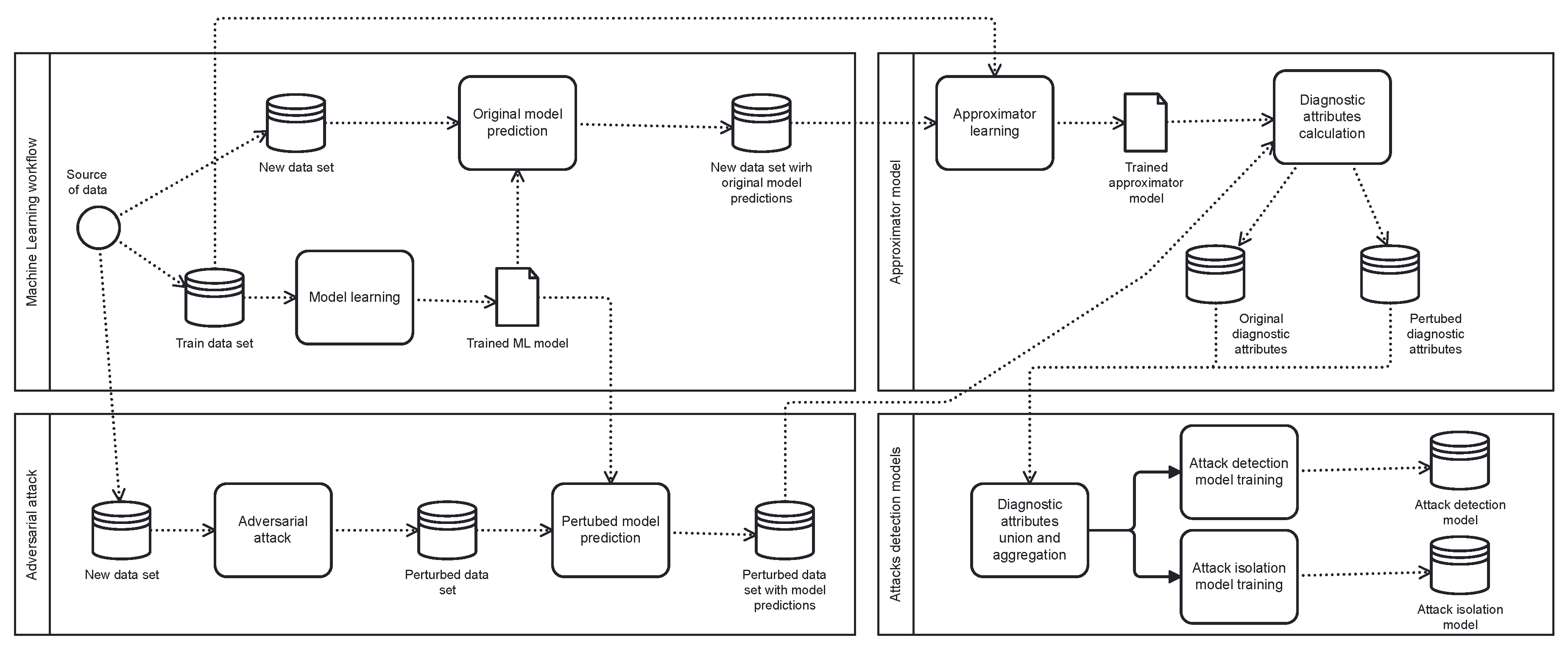
3.2. Approximator Learning

The paper [27] describes the detailed workflow associated with model approximation and diagnostic attributes; in this section we just briefly call the most important assumptions. The main idea underlying this approach is to create a surrogate model [28,29] based on predictions of the origin model $M\left(x\right)$. We expect that a surrogate model will mimic the behavior of the original model M, which we do not have access to. This assumption is due to the business environment, in which access to the original model is difficult, while our method requires only access to the training data. In addition, an approach based solely on predictions is model-agnostic and universal. The quality of a surrogate model is monitored by the Cohen kappa score calculated between the original predictions and the approximated predictions, and it should be above 0.9 for good properties. To approximate these predictions, we use the rough sets theory [30] and create a surrogate model using an ensemble of approximate reducts $AR$ [31]. An approximate reduct is an irreducible subset of attributes that is sufficient to express almost the same information about the decisions as the whole attribute set. In this context, we distinguish two data sets: diagnosed (new) $D=(X_D,d_D)$, which is used to create a surrogate model, and training $R=(X_R,d_R)$, which is used to train the original model. In our case, the decision values for which we construct the approximate reducts correspond to predictions of the diagnosed model, i.e., $M\left(X_D\right)$, not the actual ground truth target values. The result of the above-mentioned steps is the trained approximator model $\overline{M}$, composed of a set of approximate reducts $\mathcal{R}=\{A{R}_1,\dots ,A{R}_i,\dots ,A{R}_k\}$ and approximated prediction for instances of data $\overline{M}\left(x\right)$. The construction of the approximator depends on the selection of two hyper-parameters: an $ϵ$ representing the approximation threshold for reducts, and a number of reducts in the ensemble. Since the aim of the procedure is to find the appropriate approximation of the model’s predictions, we use the grid search to tune the hyper-parameter settings. We also assume that there is access to the decision attribute (target) in the data set, which will be denoted as d. For $d\left(x\right)$, we will denote its value for an instance x. Moreover, $q^M\left(x\right)$ is the estimation of decision class probabilities made by the diagnosed model M and $\overline{q^M}\left(x\right)$ is the approximation of decision class probability predictions.

The next step is defining the neighborhood $N\left(x\right)$ for each observation in the diagnosed data set. We want to identify instances that are similar with regard to predictions made by M, and we define a notion of neighborhood based on the prediction process of the model approximator $\overline{M}$. In particular, the neighborhood $N^{AR}\left(x\right)$ for a diagnosed instance x with regard to a single reduct $AR\in \mathcal{R}$ is defined as a subset of instances from $X_R$ that belong to the same indiscernibility class, i.e., ${\left[x\right]}_{AR}$. The final neighborhood is the sum of neighborhoods computed for all reducts in the ensemble. Thus, for each instance in the diagnosed data set, we have information about similar instances in the training data set. Then, it is possible to compare the distribution of targets, predictions, and approximate predictions between given observations in the diagnosed data set and similar observations from the training data set, which were chosen for the neighborhood. Such a defined neighborhood for a given observation from a diagnosed data set in extreme cases can contain all observations from the training data set or none of them. The neighborhood is the basis for calculating diagnostic attributes, which are listed below:

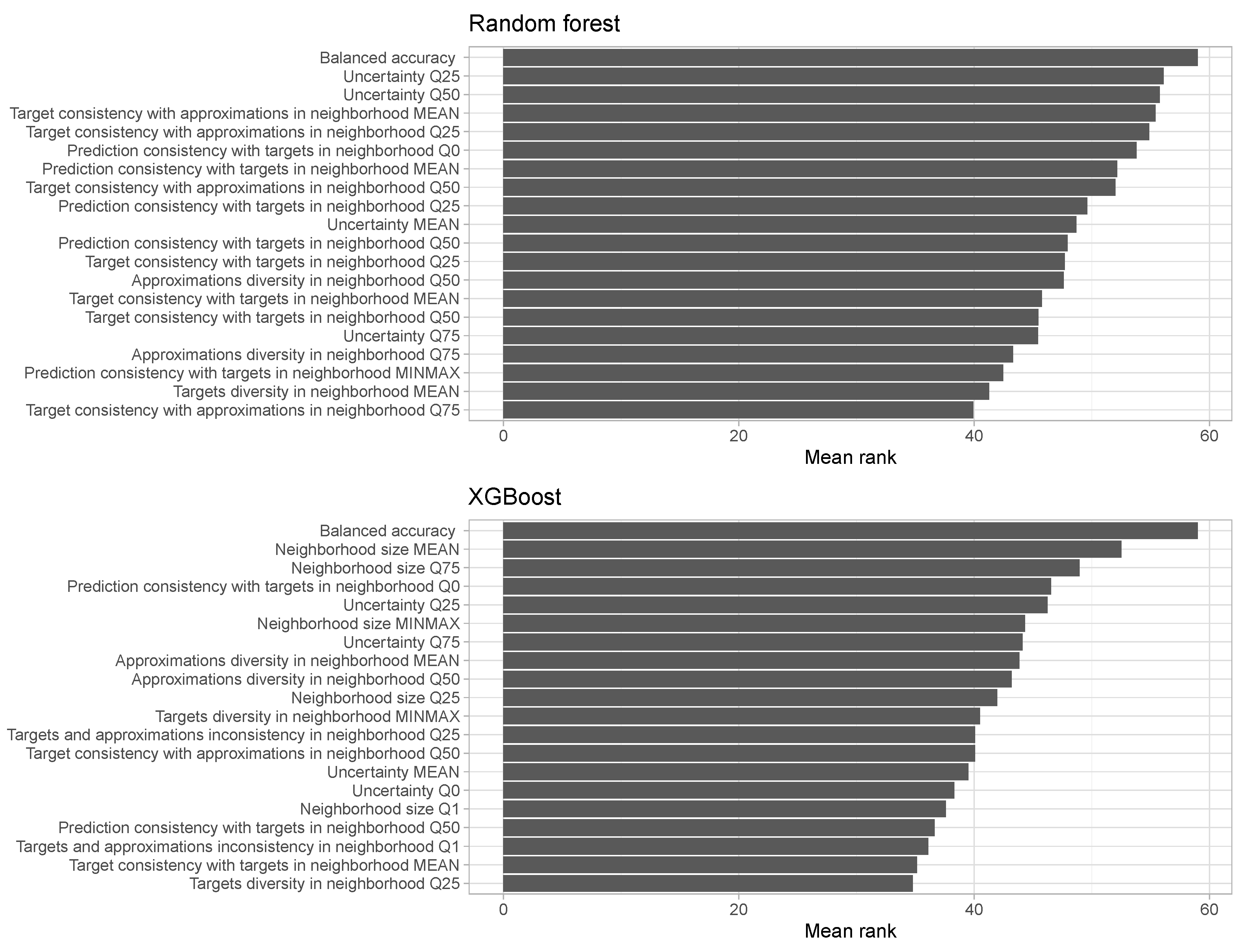
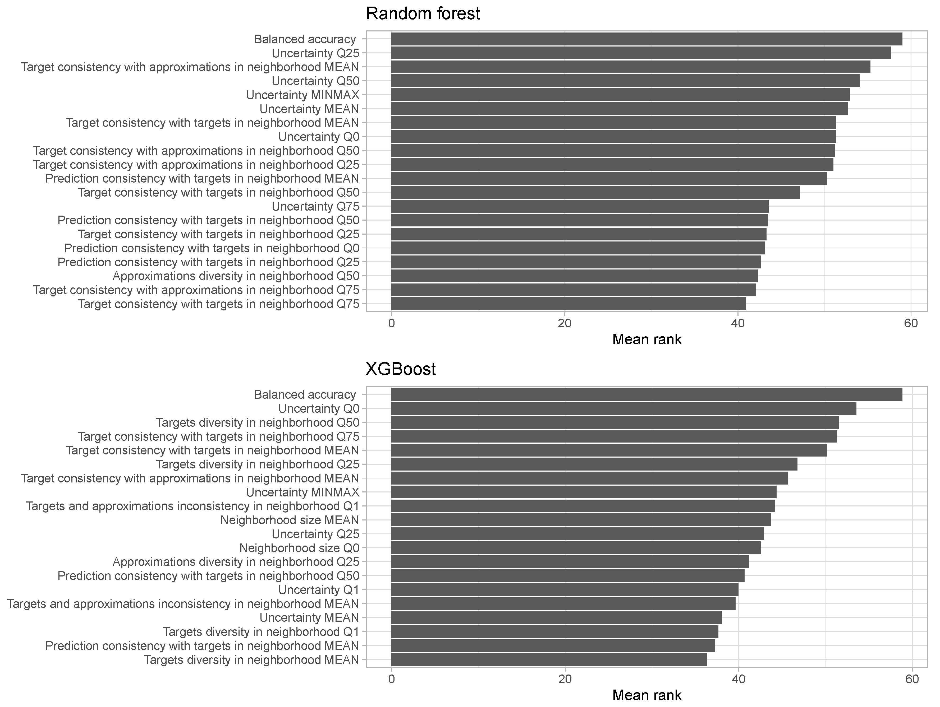
• Target consistency with approximations in the neighborhood—measures the consistency of the target of the diagnosed instance with the approximations from the neighborhood of this instance. It expresses how often values from $\overline{M}\left(N\left(x\right)\right)$ are the same as $d_x$.
• Prediction consistency with targets in the neighborhood—measures the consistency of the prediction of the diagnosed instance with the targets from the neighborhood of this instance. It expresses how often values from $d_{N\left(x\right)}$ are the same as $M\left(x\right)$.
• Target consistency with targets in the neighborhood—measures the consistency of the target of the diagnosed instance with the targets from the neighborhood of this instance. It expresses how often values from $d_{N\left(x\right)}$ agree with the class of x, i.e., $d_x$.
• Targets and approximations inconsistency in the neighborhood—measures the inconsistency of targets and approximations in the neighborhood of the diagnosed instance. This attribute is calculated as $\frac{1}{\left|N\left(x\right)\right|}{\sum }_{x^{\prime }\in N\left(x\right)}\left[1-\overline{q_{d_{x^{\prime }}}}\left(x^{\prime }\right)\right]$, where $d_{x^{\prime }}$ is the ground truth target class of $x^{\prime }$, and $\overline{q_{d_{x^{\prime }}}}$ is the approximation of its probability.
• Targets diversity in the neighborhood—measures the diversity of targets in the neighborhood of the diagnosed instance in comparison to the diversity of targets calculated on the whole diagnosed data set. It is calculated as $h(p,p(N\left(x\right)\left)\right)$, where p is the prior probability distribution of decision classes and $p\left(N\right(x\left)\right)$ is the distribution of decision classes in the neighborhood of x.
• Approximations diversity in the neighborhood—measures the diversity of approximations in the neighborhood of the diagnosed instance in comparison to the diversity of approximations calculated on the whole diagnosed data set. It refers to $h(p,\overline{q}\left(N\left(x\right)\right))$, where $\overline{q}\left(N\left(x\right)\right)$ is the distribution of the approximated predictions in $N\left(x\right)$.
• Uncertainty—we define a normalized entropy of a classification distribution $q\left(x\right)$ as $H_{norm}\left(q\left(x\right)\right)=-\frac{{\sum }_{i=1}^l{q}_i\left(x\right)log\left(q_i\left(x\right)\right)}{log\left(l\right)}$, where l is a number of classes. In a case when the prior is not uniform, we need to transform it by scaling the simplex space. Let us take the distribution norm of $q\left(x\right)$ with respect to p as ${\left|q\left(x\right)\right|}_p=\sum \frac{q_i\left(x\right)}{p_i}$. It measures the distribution $q\left(x\right)$ with the units of the prior distribution. Let us define a p-simplex off-centering as ${\left[O{C}_p\left(q_i\left(x\right)\right)\right]}_i=\frac{q_i\left(x\right)}{{p_i\left|q\left(x\right)\right|}_p}$. Then we obtain the prior-off-centered normalized entropy $OC{E}_p\left(q\left(x\right)\right)=H\left(O{C}_p\left(q\left(x\right)\right)\right)$, which, for the sake of simplicity, we will denote as $Unc\left(x\right)$, which is the prediction uncertainty of model M calculated for a diagnosed instance x.
• Neighborhood size—the number of instances in the neighborhood of the diagnosed instance.

Diagnostic attributes are a standardized format of comparing and diagnosing diverse data sets regardless of the number of classes or attributes.

4. Experiments

This section presents the results of the conducted study, in which we applied the workflow presented in Figure 1 to a variety of real data sets. Firstly, three different model architectures were fitted to each data set, and then three different adversarial attacks were conducted. Based on the obtained predictions, we prepared surrogate models and calculated the diagnostics attributes. In the next step, they were used to prepare two kinds of classifiers: for attack detection, where we wanted to predict the occurrence of an adversarial attack without distinguishing its type, and for attack isolation, where we wanted to predict also the type of the conducted adversarial attack.

4.1. Data Preparation

We obtained 22 data sets with classification tasks from OpenML. The list of data sets with basic characteristics is presented in

Table 1. Basic characteristics of data sets used in experiments.

Data Set Name	Number of Instances	Number of Attributes	Number of Classes
Bioresponse	3751	1776	2
churn	5000	20	2
cmc	2000	47	10
cnae-9	1080	856	9
dna	3186	180	3
har	10,299	561	6
madelon	2600	500	2
mfeat-factors	2000	47	10
mfeat-fourier	2000	76	10
mfeat-karhunen	2000	47	10
mfeat-zernike	2000	47	10
nomao	34,465	118	2
optdigits	2000	47	10
pendigits	10,992	16	10
phoneme	5404	5	2
qsar-biodeg	1055	41	2
satimage	6430	36	6
semeion	1593	256	10
spambase	2000	47	10
wall-robot-navigation	5456	24	4
wdbc	569	30	2
wilt	4839	5	2

.

Each data set was divided into training and diagnostic parts, with the diagnosis data set including at least 100 observations. We fit a logistic regression model, a support vector machine, and XGBoost to each data set. Following that, three adversarial attacks were launched against the diagnosed part of each data set. All calculations were conducted in Python using the Adversarial Robustness Toolbox package [32] and Permute Attack repository [18].

In the next step, we calculated diagnostic attributes for each data set and attack based on proper surrogate models. To create the surrogate models, we utilized an ensemble of 2500 approximate reducts with $ϵ$ equal to 0.05. Figure 2 shows the distribution of obtained Cohen kappa scores between the original prediction and the approximated predictions made by the surrogate model; for every data set and model type, the quality condition of the surrogate model was met. All scores are above 0.9 and the median of these values is equal to 1.

The result of approximator learning is that the data set contains values of eight diagnostic attributes for each instance of the diagnosis data set and attack. To provide suitable data for training a classifier, we aggregated these attributes within cross-sections defined by data set, model, and attack. For each diagnostic attribute, a set of descriptive statistics was calculated: mean, minimum, maximum, lower quartile, median, upper quartile, and range. For those aggregates, we also added some data set characteristics such as the number of observations, the number of classes in the classification problem, and the balanced accuracy calculated based on predictions and targets. There were a total of 59 features analyzed.

Table 2. Example of aggregated data utilized for attack detection and isolation models estimation.

Data Set	Model	Attack	Bacc	n_obs	Neigh_Size_Mean	Neigh_Size_q0	⋯
Bioresponse	lin	hsj	0.26	751.00	178.06	67.00	⋯
Bioresponse	lin	org	0.74	751.00	264.75	122.00	⋯
Bioresponse	lin	per	0.36	751.00	263.78	122.00	⋯
Bioresponse	lin	zoo	0.00	751.00	261.08	120.00	⋯
Bioresponse	svm	hsj	0.50	751.00	277.85	66.00	⋯
Bioresponse	svm	org	0.77	751.00	408.08	208.00	⋯
Bioresponse	svm	per	0.52	751.00	402.40	207.00	⋯
Bioresponse	svm	zoo	0.02	751.00	358.64	95.00	⋯
Bioresponse	xgb	hsj	0.22	751.00	178.99	77.00	⋯
Bioresponse	xgb	org	0.78	751.00	290.35	150.00	⋯
Bioresponse	xgb	per	0.31	751.00	285.49	151.00	⋯
Bioresponse	xgb	zoo	0.64	751.00	290.25	148.00	⋯
churn	lin	hsj	0.42	1000.00	9.57	2.00	⋯
churn	lin	org	0.58	1000.00	58.20	5.00	⋯
churn	lin	per	0.42	1000.00	25.49	4.00	⋯
⋯	⋯	⋯	⋯	⋯	⋯	⋯	⋯

presents the first 15 rows and 7 columns of the aggregated data set utilized for attack detection and isolation models estimation. For the attack detection problem, column attack was replaced by a binary variable equal to 0 for org value, meaning lack of attack, and 1 otherwise.

4.2. Scenarios

For assessment of the effectiveness of diagnostic attributes in attack detection and isolation, we designed a set of experiments described in

Table 3. Considered scenarios.

Scenario Name	Description	Application
10-fold cross-validation	Cross-validation stratified by variable of interest	detection, isolation
one-data-set-out	One data set is treated as a test data set and the rest of data is a training data set	detection, isolation
one-model-out	Data for one model type is treated as a test data set and the rest of data is a training data set	detection, isolation
one-attack-out	Data for one attack type is treated as a test data set and the rest of data is a training data set	detection

.

The first column of Table 3 contains the scenario name, the second provides a short description of the main idea behind the given scenario, and the third column presents information when the scenario is applicable. Each scenario except the last will be realized for both types of task—detection of attack and isolation of attack type. The last scenario is applicable only for detection because we aim to teach a model to recognize attacks, whose characteristics were not included in the training data. In each scenario, we trained random forest and XGBoost models with hyper-parameters optimization.

4.3. Attack Detection

In the first experiment, we aimed to train classifiers that distinguish only two classes—no attack versus any attack.

Table 4. Balanced accuracy with its standard deviation for each scenario in attack detection.

Scenario Name	RF	XGB
10-fold cross-validation	0.9107 (0.1050)	0.9557 (0.0679)
one-attack-out	0.9495 (0.0437)	0.9596 (0.0350)
one-data-set-out	0.9015 (0.1599)	0.9520 (0.1167)
one-model-out	0.9364 (0.0441)	0.9164 (0.0621)

presents the results of the trained models.

Regardless of model architecture, it is possible to identify an attack using diagnostic attributes. The highest balanced accuracy is obtained for a one-attack-out scenario in both classifiers. It shows that we are able to recognize the fact of attack even for previously unseen attacks. The lowest performance is observed for a one-data-set-out scenario with a random forest classifier; for a new data set, it was more difficult to identify the attack than e.g., a new model type.

For each scenario and classifier, we extracted feature importance and created the ranking of these variables—higher rank means higher importance. We calculated the correlation coefficients between these ranks and scenarios. The results show that the order of features is highly correlated within classifier groups. For example, the correlation between the feature importance ranks between 10-fold cross-validation and one-data-set-out scenarios for the random forest classifier is equal to 0.97. The correlation coefficient for XGB and RF is rather small, varying from 0.19 to 0.30. It shows that completely different variables are significant in attack identification for analyzed classifiers. Figure 3 shows the top 20 most important variables for each classifier.

The main role in both cases has a balanced accuracy calculated on the test data set. The second and third places contain an uncertainty diagnostic attribute for the random forest classifier, while for XGBoost there is the neighborhood size diagnostic attribute. The most frequent variable in the top 20 for RF is prediction consistency with targets in neighborhood, while for XGB it is neighborhood size. It shows that each diagnostic attribute contains valuable information that helps distinguish the occurrence of an attack in data.

4.4. Attack Isolation

In another experiment, we trained random forest and XGBoost classifiers to distinguish attack types. The decision variable has four classes—no attack, the HopSkipJump attack, the PermuteAttack, and the ZOO attack.

Table 5. Balanced accuracy with its standard deviation for each scenario in attack isolation.

Scenario Name	RF	XGB
10-fold cross-validation	0.6560 (0.1542)	0.7625 (0.0961)
one-data-set-out	0.7443 (0.2213)	0.8030 (0.1512)
one-model-out	0.7102 (0.1476)	0.7216 (0.1379)

shows the results of each scenario.

We can see that attack isolation has poorer performance than attack detection. Using the XGBoost model architecture, we obtain higher balanced accuracy values than for random forest. The highest values are observed for the one-data-set-out scenario. This suggests that distinguishing the attack type for the new data set is easier than for the new model type.

The analysis of feature importance ranks shows that, similar to those obtained for attack detection, they are highly correlated within the classifier type. The correlation coefficient between scenarios for the same classifier varies from 0.67 to 0.99. However, correlation values between the results of scenarios realized using RF and XGB are slightly higher than those presented in the previous section and are in the range of 0.41–0.51. Figure 4 presents the mean rank for the top 20 features used in analyzed classifiers.

In the case of attack detection as well, the most important feature is balanced accuracy, calculated on the attacked data set. In subsequent places, we can observe variables connected with uncertainty measures. In the presented top 20 most influential features, the random forest classifier uses statistics calculated based on five diagnostic attributes, while the XGBoost classifier uses eight diagnostic attributes.

5. Conclusions and Future Works

In this paper, we tested two ML models’ architecture to build classifiers for adversarial attack detection and isolation. We designed a set of scenarios that utilize a leave-one-out and cross-validation methodology to investigate whether it is possible to distinguish the occurrence of the attack and the attack type based on diagnostic attributes.

The results show that the method works and is suitable for attack detection—it is possible to build a classifier, operating on diagnostic attributes, that can detect adversarial attacks with a balanced accuracy greater than 0.9. This method works also for detecting attacks that were not included in the training data set.

For attack isolation, we obtained poorer performance of classifiers—the balanced accuracy varied from 0.66 to 0.80. The conducted research indicated the most important features used by trained classifiers: the balanced accuracy of the diagnosed data set, uncertainty, and neighborhood size.

Future works can be divided into three distinctive work streams:

• Increasing the quality of classifiers, by training them on larger representations of known attack methods and data sets. New data sets and new adversarial examples will become available as a direct result of implementation activities performed by the QED Software company and will focus on real-life examples of attacks and data in attack-prone environments.
• Testing different hierarchical approaches to the classifier construction—chaining attack detection classifiers with attack identification ones.
• Combining the resulting classifiers with external input sources explaining changes in data characteristics. This includes methods for concept drift detection, anomaly detection, and expert reasoning.

References

1. Jordan, M.I.; Mitchell, T.M. Machine learning: Trends, perspectives, and prospects. Science 2015, 349, 255–260. [Google Scholar] [CrossRef] [PubMed]
2. Ribeiro, M.T.; Singh, S.; Guestrin, C. “Why Should I Trust You?”: Explaining the Predictions of Any Classifier. In Proceedings of the 22nd ACM SIGKDD International Conference on Knowledge Discovery and Data Mining, San Francisco, CA, USA, 13–17 August 2016; Association for Computing Machinery: New York, NY, USA, 2016; pp. 1135–1144. [Google Scholar] [CrossRef]
3. Akhtar, N.; Mian, A. Threat of Adversarial Attacks on Deep Learning in Computer Vision: A Survey. IEEE Access 2018, 6, 14410–14430. [Google Scholar] [CrossRef]
4. Papernot, N.; McDaniel, P.; Goodfellow, I.; Jha, S.; Celik, Z.B.; Swami, A. Practical Black-Box Attacks against Machine Learning. In Proceedings of the 2017 ACM on Asia Conference on Computer and Communications Security, Abu Dhabi, United Arab Emirates, 2–6 April 2017; pp. 506–519. [Google Scholar] [CrossRef]
5. Carlini, N.; Wagner, D. Towards Evaluating the Robustness of Neural Networks. In Proceedings of the 2017 IEEE Symposium on Security and Privacy, San Jose, CA, USA, 22–26 May 2017; pp. 39–57. [Google Scholar] [CrossRef]
6. Liang, H.; He, E.; Zhao, Y.; Jia, Z.; Li, H. Adversarial Attack and Defense: A Survey. Electronics 2022, 11, 1283. [Google Scholar] [CrossRef]
7. Chakraborty, A.; Alam, M.; Dey, V.; Chattopadhyay, A.; Mukhopadhyay, D. A survey on adversarial attacks and defences. CAAI Trans. Intell. Technol. 2021, 6, 25–45. [Google Scholar] [CrossRef]
8. Pawlak, Z. Rough Sets: Theoretical Aspects of Reasoning About Data; Springer Science & Business Media: Dordrecht, The Netherlands, 1991. [Google Scholar]
9. Skowron, A.; Polkowski, L. Rough Sets in Knowledge Discovery 1: BASIC Concepts; CRC Press: Berlin, Germany, 1998. [Google Scholar]
10. Ren, K.; Zheng, T.; Qin, Z.; Liu, X. Adversarial Attacks and Defenses in Deep Learning. Engineering 2020, 6, 346–360. [Google Scholar] [CrossRef]
11. Kireev, K.; Kulynych, B.; Troncoso, C. Adversarial Robustness for Tabular Data through Cost and Utility Awareness. In Proceedings of the NeurIPS ML Safety Workshop, Virtual, 9 December 2022. [Google Scholar]
12. Goodfellow, I.J.; Shlens, J.; Szegedy, C. Explaining and harnessing adversarial examples. arXiv 2014, arXiv:1412.6572. [Google Scholar]
13. Szegedy, C.; Zaremba, W.; Sutskever, I.; Bruna, J.; Erhan, D.; Goodfellow, I.; Fergus, R. Intriguing properties of neural networks. In Proceedings of the International Conference on Learning Representations, Scottsdale, AZ, USA, 2–4 May 2013. [Google Scholar]
14. Biggio, B.; Roli, F. Wild Patterns: Ten Years After the Rise of Adversarial Machine Learning. In Proceedings of the 2018 ACM SIGSAC Conference on Computer and Communications Security, Toronto, ON, Canada, 15–19 October 2018; pp. 2154–2156. [Google Scholar] [CrossRef]
15. Biggio, B.; Nelson, B.; Laskov, P. Poisoning Attacks against Support Vector Machines. In Proceedings of the 29th International Conference on International Conference on Machine Learning, Edinburgh, UK, 26 June–1 July 2012; Omnipress: Madison, WI, USA, 2012; pp. 1467–1474. [Google Scholar]
16. Barreno, M.; Nelson, B.; Joseph, A.D.; Tygar, J.D. The security of machine learning. Mach. Learn. 2010, 81, 121–148. [Google Scholar] [CrossRef]
17. Chen, J.; Jordan, M.I.; Wainwright, M.J. Hopskipjumpattack: A query-efficient decision-based attack. arXiv 2019, arXiv:1904.02144. [Google Scholar]
18. Hashemi, M.; Fathi, A. PermuteAttack: Counterfactual Explanation of Machine Learning Credit Scorecards. arXiv 2020, arXiv:2008.10138. [Google Scholar]
19. Chen, P.Y.; Zhang, H.; Sharma, Y.; Yi, J.; Hsieh, C.J. Zoo: Zeroth order optimization based black-box attacks to deep neural networks without training substitute models. In Proceedings of the 10th ACM Workshop on Artificial Intelligence and Security, Dallas, TX, USA, 3 November 2017; pp. 15–26. [Google Scholar]
20. Grosse, K.; Manoharan, P.; Papernot, N.; Backes, M.; Mcdaniel, P. On the (Statistical) Detection of Adversarial Examples. arXiv 2017, arXiv:1702.06280. [Google Scholar]
21. Metzen, J.H.; Genewein, T.; Fischer, V.; Bischoff, B. Detecting adversarial perturbations with neural networks. In Proceedings of the 5th International Conference on Learning Representations, ICLR 2017, Toulon, France, 24–26 April 2017. [Google Scholar]
22. Li, T.; Wang, L.; Li, S.; Zhang, P.; Ju, X.; Yu, T.; Yang, W. Adversarial sample detection framework based on autoencoder. In Proceedings of the 2020 International Conference on Big Data & Artificial Intelligence & Software Engineering (ICBASE), Bangkok, Thailand, 30 October–1 November 2020; pp. 241–245. [Google Scholar] [CrossRef]
23. Meng, D.; Chen, H. MagNet: A Two-Pronged Defense against Adversarial Examples. In Proceedings of the 2017 ACM SIGSAC Conference on Computer and Communications Security, Dallas, TX, USA, 30 October–3 November 2017. [Google Scholar]
24. Xu, W.; Evans, D.; Qi, Y. Feature Squeezing: Detecting Adversarial Examples in Deep Neural Networks. arXiv 2018, arXiv:1704.01155. [Google Scholar] [CrossRef]
25. Papernot, N.; McDaniel, P.; Wu, X.; Jha, S.; Swami, A. Distillation as a Defense to Adversarial Perturbations Against Deep Neural Networks. In Proceedings of the 2016 IEEE Symposium on Security and Privacy, San Jose, CA, USA, 22–26 May 2016; pp. 582–597. [Google Scholar] [CrossRef]
26. Cohen, J.; Rosenfeld, E.; Kolter, Z. Certified Adversarial Robustness via Randomized Smoothing. In Proceedings of the 36th International Conference on Machine Learning, Long Beach, CA, USA, 9–15 June 2019; Volume 97, pp. 1310–1320. [Google Scholar]
27. Janusz, A.; Zalewska, A.; Wawrowski, L.; Biczyk, P.; Ludziejewski, J.; Sikora, M.; Ślęzak, D. BrightBox—A rough set based technology for diagnosing mistakes of machine learning models. Appl. Soft Comput. 2023, 141, 110285. [Google Scholar] [CrossRef]
28. Maszczyk, C.; Kozielski, M.; Sikora, M. Rule-based approximation of black-box classifiers for tabular data to generate global and local explanations. In Proceedings of the 2022 17th Conference on Computer Science and Intelligence Systems (FedCSIS), Sofia, Bulgaria, 4–7 September 2022; pp. 89–92. [Google Scholar]
29. Henzel, J.; Tobiasz, J.; Kozielski, M.; Bach, M.; Foszner, P.; Gruca, A.; Kania, M.; Mika, J.; Papiez, A.; Werner, A.; et al. Screening support system based on patient survey data—Case study on classification of initial, locally collected COVID-19 data. Appl. Sci. 2021, 11, 10790. [Google Scholar] [CrossRef]
30. Skowron, A.; Ślęzak, D. Rough Sets Turn 40: From Information Systems to Intelligent Systems. In Proceedings of the 17th Conference on Computer Science and Intelligence Systems, FedCSIS 2022, Sofia, Bulgaria, 4–7 September 2022; Volume 30, pp. 23–34. [Google Scholar] [CrossRef]
31. Stawicki, S.; Ślęzak, D.; Janusz, A.; Widz, S. Decision Bireducts and Decision Reducts—A Comparison. Int. J. Approx. Reason. 2017, 84, 75–109. [Google Scholar] [CrossRef]
32. Nicolae, M.I.; Sinn, M.; Tran, M.N.; Buesser, B.; Rawat, A.; Wistuba, M.; Zantedeschi, V.; Baracaldo, N.; Chen, B.; Ludwig, H.; et al. Adversarial Robustness Toolbox v1.2.0. arXiv 2018, arXiv:1807.01069. [Google Scholar]
Figure 1. Diagram of the analysis workflow.
Applsci 13 09698 g001
Figure 2. The Cohen kappa score for each model and data set. Different colors for models were applied to distinguish close data points.
Applsci 13 09698 g002
Figure 3. Mean rank of feature importance across classifiers for attack detection.
Applsci 13 09698 g003
Figure 4. Mean rank of feature importance across classifiers for attack isolation.
Applsci 13 09698 g004