Article

A Calibration Method for Time Dimension and Space Dimension of Streak Tube Imaging Lidar

1
National Key Laboratory of Science and Technology on Tunable Laser, Harbin Institute of Technology, Harbin 150080, China
2
Research Center for Space Optical Engineering, School of Astronautics, Harbin Institute of Technology, Harbin 150001, China
*
Authors to whom correspondence should be addressed.
Appl. Sci. 2023, 13(18), 10042; https://doi.org/10.3390/app131810042
Submission received: 18 August 2023 / Revised: 30 August 2023 / Accepted: 4 September 2023 / Published: 6 September 2023
(This article belongs to the Special Issue Advances in Optical and Optoelectronic Devices and Systems)

Abstract

:
Owing to the special working systems of streak tube imaging lidar (STIL), the time and space dimensions are coupled together on the streak images. This coupling can cause measurement errors in 3D point clouds and can make measurement results more complicated to calibrate than other kinds of lidars. This paper presents a method to generate a time calibration array and an angle calibration array to separate the offset of the streak into time dimension and space dimension. The time and space information of the signal at any position on the streak image can be indexed through these two arrays. A validation experiment on aircraft was carried out, and the range error of the 3D point cloud was improved from 0.41 m to 0.27 m using the proposed calibration method. Thus, using the proposed calibration method can improve the accuracy of the point cloud produced by STIL.

1. Introduction

With the development of different types of lidar, the three-dimensional (3D) lidar technique has been widely used in a variety of fields, including city construction, topographic mapping, underwater detection, and robotics [1,2,3,4,5]. Streak tube imaging lidar (STIL) has attracted great interest in recent years because of its wide field of view and fast data rate [6,7,8,9], which can be attributed to the detection system’s ability to obtain hundreds of returns in one laser pulse.
A typical schematic of the STIL system is shown in Figure 1. The laser is shaped into a fan beam by a cylindrical lens and forms a thin strip footprint on the target. The returned optical signal from the target is collected by the receiving optical system and imaged on the photocathode of the streak tube, and then the optical signal is converted into electrons. When the electron beam is accelerated toward the phosphor screen by a high voltage between the two ends of the streak tube, it is deflected by a pair of linear sweep voltages. Finally, the electrons hit the screen of the streak tube and form a streak image [10]. The signature position in a time-resolved channel on the screen is relative to the arrival time of the signal; that is, we can obtain the target distance from the image [11,12,13]. Usually, images are intensified by a microchannel plate(MCP) and recorded by a charge-coupled device (CCD) [14,15]. The horizontal position represents the spatial information of the target, while the vertical position represents the distance information in Figure 1.
However, certain problems can occur in practice. For example, it is difficult to deconstruct the offset of a streak on the CCD into time and space dimensions because of the diffusion of the optical imaging system and electronic imaging system [16,17], non-parallelism between the direction of the sweep electric field and the direction of time-resolved channels, the installation angle difference of the CCD and streak tube, and other factors.
Thus, improving the temporal and spatial resolution of streak tubes has remained a topic of concern to researchers [18,19,20]. This work presents a method to generate a time calibration array and an angle calibration array to separate the offset of a streak into a time dimension and a space dimension. The method aims to improve the range accuracy of the point cloud produced by STIL through the correction of the two calibration arrays.

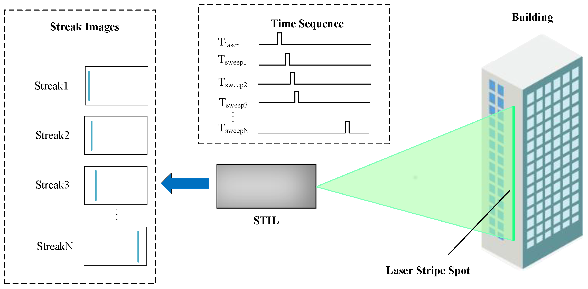
2. Coupling Mechanism

Different from other types of lidars, our approach features detection data (i.e., streak images) containing both time and space information. Ideally, the streak contains some illuminated pixels on the CCD. The position of the streak on the time axis is used to calculate the time when the echo signal reaches the detector, and the distance of the target can be calculated based on the propagation speed of light in the air. Generally, we obtain the position of the streak by calculating its centroid on the time axis [10]:
x j = i = 1 N ( i × I i ) i = 1 N I i
where xj is the centroid of the pixels of the jth row, N is the number of pixels in the time dimension of the CCD, and Ii is the gray value of the ith pixel. Afterward, we obtain the distance of the point on the target by
R j = 1 2 c ( α x j + t d + t i n h )
where Rj is the distance of the point corresponding to the pixels of the jth row, α is a coefficient used to indicate the time represented by one pixel, td is the gate delay of the detection system, and tinh is the inherent delay of the lidar.
However, in practice, coordinates on both axes have components on the time axis and space axis. Two main reasons for this result are (1) the angle difference of the direction of the sweep electric field and the direction of the time-resolved channels on the CCD and (2) the diffusion of the optical imaging system and electronic imaging system.
The effect process of the first reason is shown in Figure 2. When there is an angle difference between the direction of the sweep electric field and the direction of the time-resolved channels on the CCD, a deviation of the dynamic streak occurs, which is shown in Figure 2a. The streak image recorded by the CCD is shown in Figure 2b.
Without the action of sweeping voltage, the position of the streak (called static streak) is as shown in Figure 2a. While the sweeping voltage is applied, the streak (called dynamic streak) is displaced along the opposite direction of the electric field. If the direction of the electric field is parallel to the time-resolved channels of the CCD, the dynamic streak is as shown in the thin green line in Figure 2a. If, however, a deflection of the direction of the electric field occurs, the dynamic streak shifts not only in the time-resolved direction but also in the space-resolved direction. As shown in Figure 2b, one pixel of the static streak is marked with a darker color and moved to the position of the pixels marked with the color red or green under the influence of the electric field. The green pixel corresponds to the black pixel when the electric field is parallel to the time-resolved channel, and the red pixel corresponds to the black pixel when there is an electric field angle. We find that when the red pixel is displaced on both the time-resolved and space-resolved channels, difficulties arise when deconstructing the position of the streak into time and space information.
Another factor leading to components on the time axis and space axis is the diffusion of the optical imaging system and electronic imaging system. An experiment was conducted to demonstrate the impact process. A laser beam with upright incidence was directed at a flat target, and the laser spot on the target could be transformed into a small point with a size of 1 mm × 1 mm by adjusting the optical emission unit. We detected the laser spot by a CCD, and the detection result is shown in Figure 3.
According to imaging principles, it is theoretically possible for only one pixel of the CCD can be lit, disregarding the diffusion of the optical imaging system and electronic imaging system. This occurrence is contingent upon factors such as the size of the laser spot, the distance between the CCD and the target, the size of a CCD pixel, and the focal length of the receiving lens. However, more than 100 pixels were actually lit up with different intensities, as shown in Figure 3.
Since the two factors work together, the deconstruction of two components on the time axis and space axis is more complex. If this problem cannot be solved, the range and spatial accuracy of STIL will be reduced.

3. Calibration Method

In this section, we will use the method of calibrating time and angle separately. The first step is time calibration, and the second step is angle calibration. Moreover, each step includes two parts: calibration experiments and data processing.

3.1. Time Calibration

3.1.1. Time Calibration Experiment

For the convenience of later expression, the time calibration experiment is referred to as Experiment I.
The effect of time calibration directly affects the range accuracy of the lidar. This paper proposes a method of gradually changing the delay of sweeping voltage to calibrate the time information corresponding to the position of the signal on the CCD. The process of the time calibration experiment is shown in Figure 4: (1) we chose a suitable experimental target, like a tall building with a height greater than the size of the light spot; the building has a flat part without windows to obtain a smooth streak signal on the CCD that is not affected by changes in the target distance; (2) we turned on the lidar to start working and adjusted the delay time of the sweeping voltage so that the streak signal would be on one edge of the image; and (3) we adjusted the delay time of the sweeping voltage step by step to move the streak to the other edge of the image. Every time a step was changed, 2000 images were recorded.
In this experiment, one step of the delay was 10 ns; more intensive detection was also possible, but overly sparse detection was not feasible. Later on, we aimed to achieve a calibration resolution of 0.1 ns through interpolation, but sparse data would affect the accuracy of interpolation results. Thus, 2000 images were recorded with the same delay to take the average and reduce the impact of the jitters from the detection system, time-sequence control unit, atmospheric disturbances, etc. After data processing, we could obtain the corresponding time information of the signal based on its position on the image. Because the streak image of the building was smooth, except for the known angles at both ends of the stripe image, the absence of angle information at other positions is uncertain. Based solely on this experiment, we were still unable to achieve angle calibration.

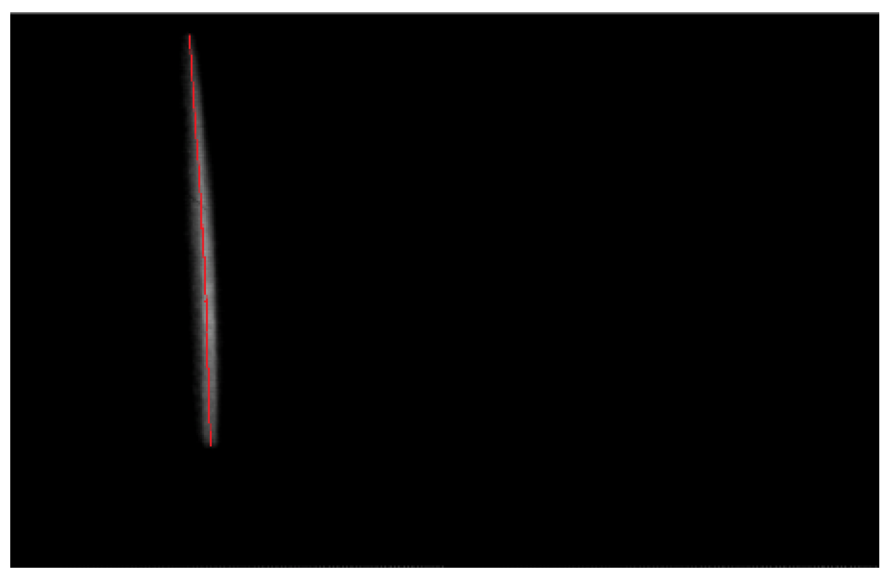
3.1.2. Data Processing for Time Calibration

In Experiment I, the data were only used for time calibration, and angle calibration was not considered. For each streak image, the centroid of the streak signal in every row could be obtained by Equation (1). The data processing results are shown in Figure 5, where the red line is composed of the centroids of each row.
By taking the average of all centroids (2000 in this work) in the same row under the same delay, we could obtain a more accurate delay centroid relationship of lidar, as shown in Figure 6.
x j = 1 S s = 1 S x j , s
In Equation (3), x j is the average of the centroids in the jth row; S is the number of streak images with the same delay time of sweeping voltage; S = 2000 here; and xj,s is the centroid in the jth row of the sth image.
As shown in Figure 6, we can find that the accidental error of the centroid of the measurement results was still relatively large, with a standard deviation of 0.84 ns, so it was necessary to reduce the error by calculating the average value.
After taking all of the average values under every delay, we could obtain a series of curves under different delays, as shown in Figure 7.
In Figure 7, one curve represents the position of the streak signal on the image under one delay value. These curves were used as a time calibration array for lidar data calibration. However, the points on adjacent curves were separated by 10 ns, and the resolution was not high enough. Therefore, we had to interpolate these curves so that the points on adjacent curves could be separated by 0.1 ns in this work.
From Figure 7, it can be found that the curvature of the rightmost curve differs greatly from other curves because the highest sweeping voltage was not high enough and because the distortion of the electronic focusing system was more serious at the edges than at other positions. Fortunately, the streak signal hardly appeared at the edge of the image, so the distorted curvature had little effect on the experimental results.

3.2. Angle Calibration Experiment

3.2.1. Angle Calibration Experiment

For the convenience of later expression, the angle calibration experiment was later referred to as Experiment II, and the process of Experiment II is shown in Figure 8.
A Leica Nova MS60 multistation was used to record the angles at both ends of the laser footprint on the building in the last experiment. To obtain spot-shaped light more conveniently, we needed an auxiliary laser to perform the experiment, and the laser of lidar was not turned on. Afterward, the laser beam was formed into a point shape and reflected onto the target by a mirror fixed on a rotating platform. The path of laser is shown by the green arrows in the figure; the red arrows indicate the direction of rotation of the mirror, the direction of light spot movement caused by rotation, and the order of streak pattern generation; while the yellow arrows indicate the change of the delay of sweeping voltage and the resulting position change of the streak signals in the images. The laser spot was moved from top to bottom, step by step, on the building along the lineation of the laser footprint of the last experiment by rotating the reflecting mirror, and during this process, the Leica Nova MS60 was used to record the current angle of the laser spot for each step of angle change. In every rotation, the delay time of sweeping voltage should be changed step by step to move the point-shape streak signal from one edge of the image to another edge. The angle change step in this experiment was 0.1 degrees, and the delay change step was 10 ns.
In the experiment, relative to the distance of the building, the Leica Nova MS60 had to be close enough to the lidar so that the error introduced by different positions of the multistation and lidar could be ignored; otherwise, it had to be eliminated through coordinate transformation between the coordinate system of the total station and the coordinate system of the lidar.
Under the same delay and angle, we recorded 2000 images to take the average and reduce the influence of jitter. This jitter was mainly imaging jitter in the space dimension, which was different from the previous experiment, where the jitter in the previous experiment was mainly imaging jitter in the temporal dimension. We calculated the centroid of every image and obtained the average value of the centroid under the same delay and angle; thus, more accurate angle information of the signal could be obtained based on its position on the image.
The time calibration information was also included in the data of Experiment II. The purpose of conducting Experiment I was to show that the light source used in Experiment I was the laser of lidar and that the coordination of the time sequential between the detector and the laser was better than that between the detector and the auxiliary laser in Experiment II. Therefore, the time accuracy of Experiment I was better. If the data from Experiment II had been used for time calibration, there would have been a significant error. As evidence, we calculated the standard deviation of two experiments, with Experiment 1 being 0.84 ns and Experiment 2 being 2.52 ns.

3.2.2. Data Processing for Angle Calibration

A calibration array is also needed, as with the time calibration. At first, we should calculate the centroid coordinates of the laser-point streak detected in Experiment II. The centroid coordinate is expressed by (x, y)
x = p = 1 P ( x p × I p ) p = 1 P I p y = p = 1 P ( y p × I p ) p = 1 P I p
where P is the number of all pixels of the CCD (655,360, i.e., 1280 × 512, in this work), Ip is the gray value of the pth pixel on the streak image, xp is the horizontal coordinate of the pth pixel, and yp is the vertical coordinate of the pth pixel. In this experiment, the horizontal axis is the time axis, and the vertical axis is the spatial axis. The horizontal and vertical coordinates are the sequence number of the pixel on the time-resolved axis and the sequence number on the space-resolved axis. The calculation results are shown in Figure 9. Different from Equation (1), which is the centroid of a row, Equation (4) is the centroid of the whole image. Moreover, threshold denoising was required for the image before extracting the centroid.
Similarly to Equation (3) and Figure 7, we took the average of the horizontal and vertical coordinates of all centroids under the same delay and angle to reduce the calibration error, and one of the averages is shown in Figure 10. The black points are the centroids, and the green star is the average of the centroids.
After taking all of the average values under every delay and angle, we obtained a series of points that filled the entire area of interest, as shown in Figure 11. We can find that the arrangement of these points was not horizontal or vertical, and the spacing between points was also different because of optical and electronic imaging diffusion and distortion. This phenomenon explains why STIL requires calibration.
Figure 11 shows the result after thinning because an overly dense point array is not conducive to observing the arrangement phenomenon described in the previous paragraph. However, during the actual calibration process, we aimed to obtain a denser matrix by two-dimensional interpolation, such that a point that falls at any position on CCD can be indexed to its angle value. We found that these points had both angle and time information, but we did not use these points for time calibration because the light source was an auxiliary laser rather than the laser of the lidar. There is a time jitter that cannot be ignored between the auxiliary laser and the lidar.

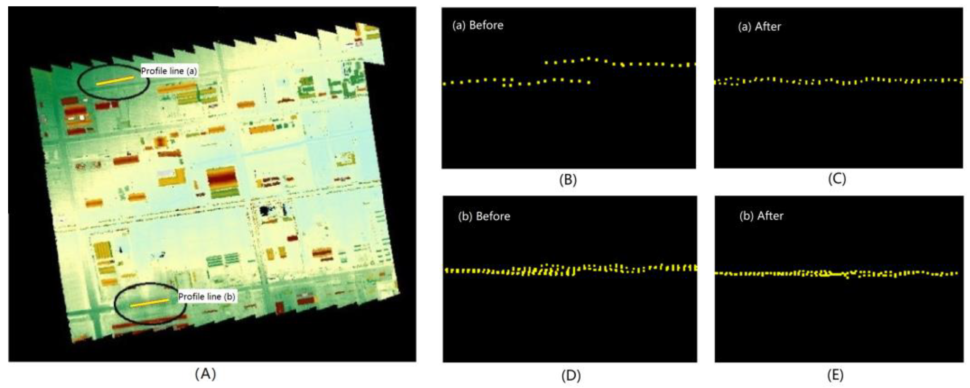
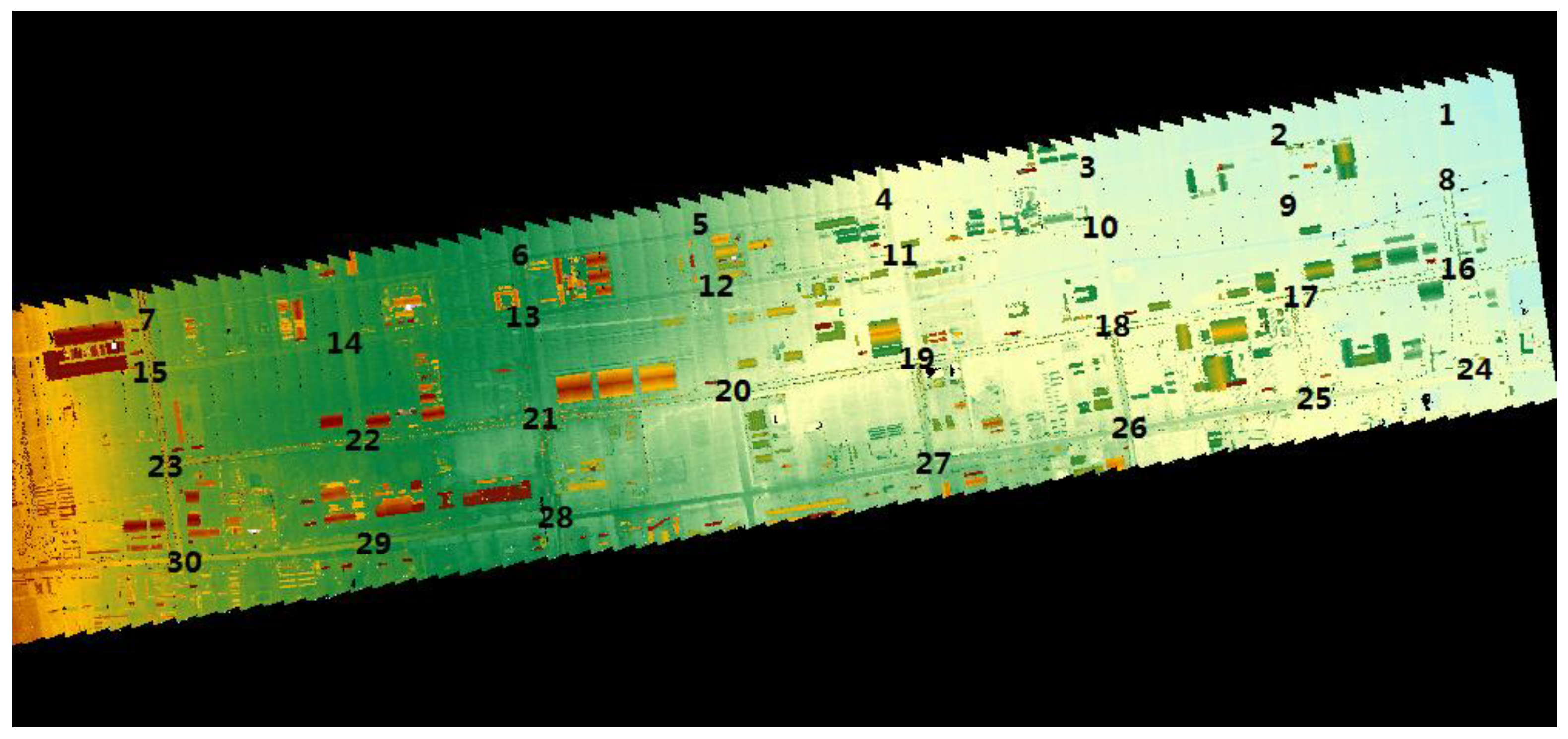
4. Calibration Results

To verify the effectiveness of the calibration method proposed in this paper, we carried out a 3D topographic mapping experiment by airborne STIL.
The aircraft flew at an altitude of about 2000 m and a speed of about 70 m/s; the terrain was relatively flat, with an elevation of about 100 m, and the surveying area was a small town in northern China. After the same data processing operation as below, filtering noise, calibrating the installation angle of the inertial measurement unit and optical system, and correcting the inherent error in distance measurement, we compared the data of the 3D point cloud before and after the time and angle calibration proposed in this paper. The results are shown in Figure 12 and Figure 13.
Differently from the push broom scanning used in traditional STIL, we used a pendulum broom scanning method [21]. Due to the fact that the streak tube detection system could be seen as a linear array detector, the point cloud was composed of individual bands. From Figure 12, we can find that the overlapping effect of the two bands was better at the profile lines after calibration. Before calibration, even if the measured ground was flat, its streak signal was irregularly curved, and the curvature of streak targets at different distances was also different. After calibration, the streak signal on the flat ground became smooth, and the splicing parts of the 3D point cloud overlapped better.
To evaluate the measurement errors before and after calibration, we measured the geographic coordinates of the 30 points listed in Figure 13 with a Leica Viva GS16 GNSS receiver. We took the measurement results of Leica Viva GS16 as the reference values and compared the point cloud data with them. We found that the range error (here, the root mean square error) of the point cloud after calibration was reduced from 0.41 m to 0.27 m.

5. Conclusions

In conclusion, we proposed a calibration method for the time dimension and space dimension of STIL. Through this method, we obtained two calibration arrays, and more accurate time and angle information can be indexed through these two arrays. Finally, we conducted a validation experiment. The experimental results indicate that the time and angle calibration method proposed in this paper is effective. The overlapping effect and the range accuracy are all improved, especially with a 34% reduction in the range error. Higher-ranging accuracy is more conducive to improving the practicality of the 3D point cloud, such as target recognition, plant growth status monitoring, vehicle quantity statistics, etc. Therefore, reducing the error by 34% is of great significance for the application of STIL. The correction method proposed in this article can effectively reduce the errors caused by the temporal and spatial coupling caused by the STIL special mechanism. The improvement of detection accuracy will play a positive role in the promotion of STIL.

Author Contributions

Conceptualization and methodology, Z.C. and R.F.; software, X.W. and C.D.; validation, Z.C., F.S. and Z.D.; data analysis, Z.C., X.W. and D.C.; writing—original draft preparation, Z.C. and F.S.; writing—review and editing, Z.C. and Z.F.; project administration, D.C. All authors have read and agreed to the published version of the manuscript.

Funding

This work was supported by the National Natural Science Foundation of China (No. 62305085 and No. 62193277012).

Institutional Review Board Statement

Not applicable.

Informed Consent Statement

Not applicable.

Data Availability Statement

According to the requirements of the project regulatory department, streak images and point cloud data cannot be provided.

Conflicts of Interest

The authors declare no conflict of interest.

References

  1. Cheng, L.; Wang, Y.; Chen, Y.; Li, M. Using LiDAR for digital documentation of ancient city walls. J. Cult. Herit. 2016, 17, 188–193. [Google Scholar] [CrossRef]
  2. Du, M.; Li, H.; Roshanianfard, A. Design and Experimental Study on an Innovative UAV-LiDAR Topographic Mapping System for Precision Land Levelling. Drones 2022, 6, 403. [Google Scholar] [CrossRef]
  3. Jantzi, A.; Jemison, W.; Illig, D.; Mullen, L. Spatial and temporal domain filtering for underwater lidar. J. Opt. Soc. Am. A 2021, 38, B10–B18. [Google Scholar] [CrossRef] [PubMed]
  4. Collings, S.; Martin, T.J.; Hernandez, E.; Edwards, S.; Filisetti, A.; Catt, G.; Marouchos, A.; Boyd, M.; Embry, C. Findings from a Combined Subsea LiDAR and Multibeam Survey at Kingston Reef, Western Australia. Remote Sens. 2020, 12, 2443. [Google Scholar] [CrossRef]
  5. Palacin, J.; Martinez, D.; Rubies, E.; Clotet, E. Mobile Robot Self-Localization with 2D Push-Broom LIDAR in a 2D Map. Sensors 2020, 20, 2500. [Google Scholar] [CrossRef] [PubMed]
  6. Tian, L.; Shen, L.; Xue, Y.; Chen, L.; Chen, P.; Tian, J.; Zhao, W. 3-D Imaging Lidar Based on Miniaturized Streak Tube. Meas. Sci. Rev. 2023, 23, 80–85. [Google Scholar] [CrossRef]
  7. Sun, J.; Wang, Q. 4-D image reconstruction for Streak Tube Imaging Lidar. Laser Phys. 2009, 19, 502–504. [Google Scholar] [CrossRef]
  8. Wei, J.; Wang, Q.; Sun, J.; Gao, J. High-resolution imaging of long-distance target with a single-slit streak-tube lidar. J. Russ. Laser Res. 2010, 31, 307–312. [Google Scholar] [CrossRef]
  9. Li, W.; Guo, S.; Zhai, Y.; Han, S.; Liu, F.; Lai, Z. Occluded target detection of streak tube imaging lidar using image inpainting. Meas. Sci. Technol. 2021, 32, 045404. [Google Scholar] [CrossRef]
  10. Ye, G.; Fan, R.; Lu, W.; Dong, Z.; Li, X.; He, P.; Chen, D. Depth resolution improvement of streak tube imaging lidar using optimal signal width. Opt. Eng. 2016, 55, 103112. [Google Scholar] [CrossRef]
  11. Gleckler, A.D. Multiple-Slit Streak Tube Imaging Lidar (MS-STIL) applications. In Proceedings of the Conference on Laser Radar Technology and Applications V, Orlando, FL, USA, 26–28 April 2000; pp. 266–278. [Google Scholar]
  12. Gleckler, A.D.; Gelbart, A.; Bowden, J.M. Multispectral and hyperspectral 3D imaging lidar based upon the multiple slit streak tube imaging lidar. In Proceedings of the Conference on Laser Radar Technology and Applications VI, Orlando, FL, USA, 13–17 April 2001; pp. 328–335. [Google Scholar]
  13. Gao, J.; Han, S.; Liu, F.; Zhai, Y.; Dai, Q.; Shimura, T. Streak tube imaging system based on compressive sensing. In Proceedings of the Conference on Optoelectronic Imaging and Multimedia Technology V, Beijing, China, 11–12 October 2018; Volume 10817. [Google Scholar]
  14. Eagleton, R.T.; James, S.F. Dynamic range measurements on streak image tubes with internal and external microchannel plate image amplification. Rev. Sci. Instrum. 2003, 74, 2215–2219. [Google Scholar] [CrossRef]
  15. Xu, Y.; Xu, T.; Liu, H.; Cai, H.; Wang, C. Gain regulation of the microchannel plate system. Int. J. Mass Spectrom. 2017, 421, 234–237. [Google Scholar]
  16. Li, H.; Chen, P.; Tian, J.; Xue, Y. High time-resolution detector based on THz pulse accelerating and scanning electron beam. Acta Phys. Sin.-CH 2022, 71, 028501. [Google Scholar] [CrossRef]
  17. Li, X.; Gu, L.; Zong, F.; Zhang, J.; Yang, Q. Temporal resolution limit estimation of x-ray streak cameras using a CsI photocathode. J. Appl. Phys. 2015, 118, 083105. [Google Scholar] [CrossRef]
  18. Tian, L.; Shen, L.; Li, L.; Wang, X.; Chen, P.; Wang, J.; Zhao, W.; Tian, J. Small-size streak tube with high edge spatial resolution. Optik 2021, 242, 166791. [Google Scholar] [CrossRef]
  19. Tian, L.; Shen, L.; Chen, L.; Li, L.; Tian, J.; Chen, P.; Zhao, W. A New Design of Large-format Streak Tube with Single-lens Focusing System. Meas. Sci. Rev. 2021, 21, 191–196. [Google Scholar] [CrossRef]
  20. Li, S.; Wang, Q.; Liu, J.; Guang, Y.; Hou, X.; Zhao, W.; Yao, B. Research of range resolution of streak tube imaging system. In Proceedings of the Conference on 27th International Congress on High-Speed Photography and Photonics, Xi’an, China, 17–22 September 2006; p. 6279. [Google Scholar]
  21. Yan, Y.; Wang, H.; Song, B.; Chen, Z.; Fan, R.; Chen, D.; Dong, Z. Airborne Streak Tube Imaging LiDAR Processing System: A Single Echo Fast Target Extraction Implementation. Remote Sens. 2023, 15, 1128. [Google Scholar] [CrossRef]
Figure 1. The schematic of the STIL system. (a) Schematic diagram of the data collection process. (b) The work principle of the streak array detector. (c) The streak image on the CCD.
Applsci 13 10042 g001
Figure 2. The coupling caused by angle difference. (a) The angle difference of the direction of the sweep electric field. (b) The streak image on the CCD.
Applsci 13 10042 g002
Figure 3. The streak image of STIL under the influence of diffusion.
Applsci 13 10042 g003
Figure 4. Time calibration experiment.
Applsci 13 10042 g004
Figure 5. The centroids of streak image.
Applsci 13 10042 g005
Figure 6. The average of all centroids under the same delay.
Applsci 13 10042 g006
Figure 7. The centroid curves under different delays.
Applsci 13 10042 g007
Figure 8. Angle calibration experiment.
Applsci 13 10042 g008
Figure 9. The centroid of the streak of the laser point in Experiment II.
Applsci 13 10042 g009
Figure 10. The centroid of the streak of the laser point.
Applsci 13 10042 g010
Figure 11. The centroid points after thinning under different delays and angles.
Applsci 13 10042 g011
Figure 12. (A) Three-dimensional point cloud of a town, (B) the section at profile line (a) before calibration, (C) the section at profile line (a) after calibration, (D) the section at profile line (b) before calibration, and (E) the section at profile line (b) after calibration.
Applsci 13 10042 g012
Figure 13. Three-dimensional point cloud of the measuring area.
Applsci 13 10042 g013
Disclaimer/Publisher’s Note: The statements, opinions and data contained in all publications are solely those of the individual author(s) and contributor(s) and not of MDPI and/or the editor(s). MDPI and/or the editor(s) disclaim responsibility for any injury to people or property resulting from any ideas, methods, instructions or products referred to in the content.

