
PSI Analysis of Adversarial-Attacked DCNN Models

1
Department of Electronics, Chungwoon University, Incheon 22100, Republic of Korea
2
Department of AIOT, Sangmyung University, Seoul 03016, Republic of Korea
*
Author to whom correspondence should be addressed.
Appl. Sci. 2023, 13(17), 9722; https://doi.org/10.3390/app13179722
Submission received: 15 July 2023
/
Revised: 21 August 2023
/
Accepted: 23 August 2023
/
Published: 28 August 2023
(This article belongs to the Special Issue AI, Machine Learning and Deep Learning in Signal Processing)
Abstract
:In the past few years, deep convolutional neural networks (DCNNs) have surpassed human performance in tasks related to recognizing objects. However, DCNNs are also threatened by performance degradation due to adversarial examples. DCNNs are essentially black-boxed, and it is not known how the output is determined internally; consequently, it is not known how adversarial attacks cause performance degradation inside the DCNNs. To observe the internal neuronal activities of DCNN models for adversarial examples, we analyzed the population sparseness index (PSI) values at each layer of two representative DCNN models, namely AlexNet and VGG11. From the experimental results, we observed that the internal responses of the two DCNN models to adversarial examples exhibited distinct layer-wise PSI values, differing from the internal responses to benign examples. The main contribution of this study is the discovery of significant differences in the internal responses of two specific DCNN models to adversarial and benign examples by PSI. Furthermore, our research has the potential not only to contribute to the design of more robust DCNN models against adversarial examples but also to bridge the gap between the fields of artificial intelligence and neurophysiology of the brain.
1. Introduction
Advances in deep convolution neural networks (DCNNs) in the field of object recognition have surpassed human-level performance [1,2]. The effective functioning of DCNNs can be attributed mainly to their structures, comprising a series of convolutional layers and fully connected layers. Each layer contains numerous units equipped with diverse filters (referred to as neurons in DCNNs), mirroring the hierarchical arrangement seen in the visual stream’s ventral layers of primates [3]. By employing this hierarchical design and utilizing supervised learning on an extensive set of object examples, DCNNs are anticipated to form intricate internal representations of external objects.
While DCNN models exhibit normal behavior on benign examples through the training process, they have a fatal disadvantage in that their performance is degraded by adversarial attacks. Adversarial examples, which are instances characterized by a small, virtually imperceptible perturbation, can cause DCNN models to make mistakes [4,5]. To human eyes, adversarial examples seem identical to the original and do not affect the perception of an object.
To DCNNs, however, they work almost as an optical illusion, causing them to misclassify data and make false predictions [6]. It is interesting to note that only DCNN models that mimic the primate visual system are sensitive to adversarial attacks [7]. Adversarial attacks reveal a serious vulnerability in deep learning systems and pose a safety challenge that cannot be ignored in AI applications [8].
However, current research cannot find a clear cause of how adversarial attacks affect deep learning systems, and only individual defense mechanisms against specific adversarial attacks have been proposed [9,10,11,12]. Analyzing the fundamental cause of adversarial attacks can help researchers to effectively overcome the vulnerability of the DCNNs. The vulnerability of DCNNs to adversarial attacks has led to a variety of opinions. While Goodfellow et al. [4] discovered that the effectiveness against such attacks did not show significant improvement, other researchers [5] put forth the hypothesis that the extreme non-linearity of DCNNs is responsible for adversarial attacks.
Conversely, even in high-dimensional linear models, adversarial attacks can confidently create successful perturbations in inputs [13]. Goodfellow et al. [4] attributed the origin of adversarial attacks to the linear characteristics exhibited in high-dimensional space. Consequently, we know very little about the process of finding the right answer within DCNNs for even benign examples. Nor do we know what happens internally when adversarial examples are applied to DCNN models [13,14,15].
Recently, an interesting study has been published related to neuronal activity in DCNNs [16]. This study demonstrated the distribution of active neurons in layers using PSI in the normal operation of DCNNs due to benign examples. PSI is a measure that allows for the representation of the sparsity of neuron activation by observing the activation status of a given neuron in the cerebral cortex when it is stimulated [17]. If we consider the nodes of each layer that constitute the DCNN model as neurons, measuring the PSI in each layer allows us to infer the internal dynamics of the models [18].
In their experiments, the distribution of PSI values for the object categories in each layer of the AlexNet and VGG11 models was analyzed, and the sparseness of neuronal activities was assessed by the PSI for the object categories of the ImageNet and Catlec256 datasets on a per-layer basis, separately. While their research made a significant contribution by employing the PSI to analyze the internal dynamics of DCNN models, their experiments were limited to cases where models function correctly on datasets composed of benign examples. Separately, our focus lies in analyzing the internal behavior of DCNN models when exposed to abnormal examples, specifically adversarial examples.
Our main idea is that there will be distinct changes in the PSI analysis compared to when benign examples are applied, when the internal dynamics of DCNN models behave differently for adversarial examples. The hypothesis within our main idea implies that the neurons in each layer of DCNN models operate abnormally when subjected to adversarial examples. To test our hypothesis, we applied the same DCNN models as in the study by [16], with the exception that we used adversarial examples instead of benign examples.
We employed three different adversarial attacks to generate adversarial examples for the experiments: FGSM attack, PGD attack, and CW attack [19]. In our experiment, we analyzed the distribution of the PSI at each layer in DCNNs for adversarial examples. Also, we compared the experimental results in [16] with our findings on the changes in the PSI according to the adversarial examples. In particular, we systematically assessed the layer-by-layer sparsity in the featured objects. Subsequently, we delineated the operational aspects of sparsity by investigating how sparsity correlates with performance at each layer. Lastly, we scrutinized the factors influencing the encoding scheme.
This paper is organized as follows: Section 2 is divided into four subsections related to the experimental setup. Section 2.1 provides descriptions of the visual image datasets used in the experiments, namely the ImageNet dataset and the Caltech256 dataset. Section 2.2 explains the architectures of the two DCNN models utilized in the experiments, namely the AlexNet and VGG11 models. In Section 2.3, we elucidate the formulation and significance of the PSI, a method employed to interpret the internal structure of DCNN models. Section 2.4 describes the attack techniques used to generate the three types of adversarial examples employed in the experiments. In Section 3, we conduct PSI analysis on the two DCNN models on a per-layer basis and analyze the implications of the findings. Lastly, we conclude the study, outline its limitations, and propose future research directions in Section 4.
2. Materials and Methods
2.1. Visual Image Datasets
For the experiment, two image datasets were prepared: the ImageNet dataset and the Caltech256 dataset as in Table 1. The dataset from ImageNet Large-Scale Visual Recognition Challenge 2012 (ILSVRC2012) [20] contains 1000 categories that are organized according to the hierarchy of WordNet [21]. The 1000 object categories consist of both internal nodes and leaf nodes of WordNet but do not overlap with each other. The dataset contains 1.2 million images for model training, 50,000 images for model validation, and 100,000 images for model testing.
In the present study, only the validation dataset (i.e., 1000 categories × 50 images) was used to evaluate the coding scheme of the DCNNs. The Caltech256 dataset consists of 30,607 images from 256 object categories with a minimum number of 80 images per category [21]. Caltech-256 is widely used for training and testing in the field of machine learning, particularly for object recognition tasks. In the present study, a selection of 80 images per category was made at random from the original dataset.
2.2. Pretrained DCNN Models
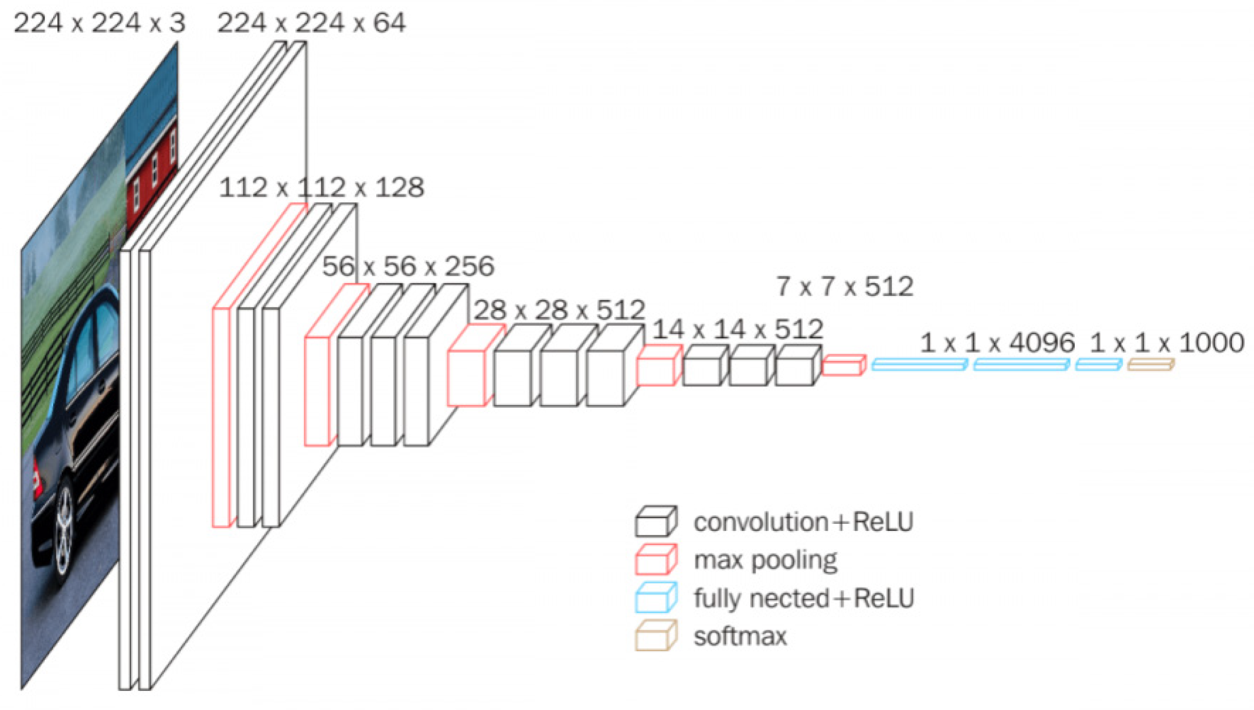
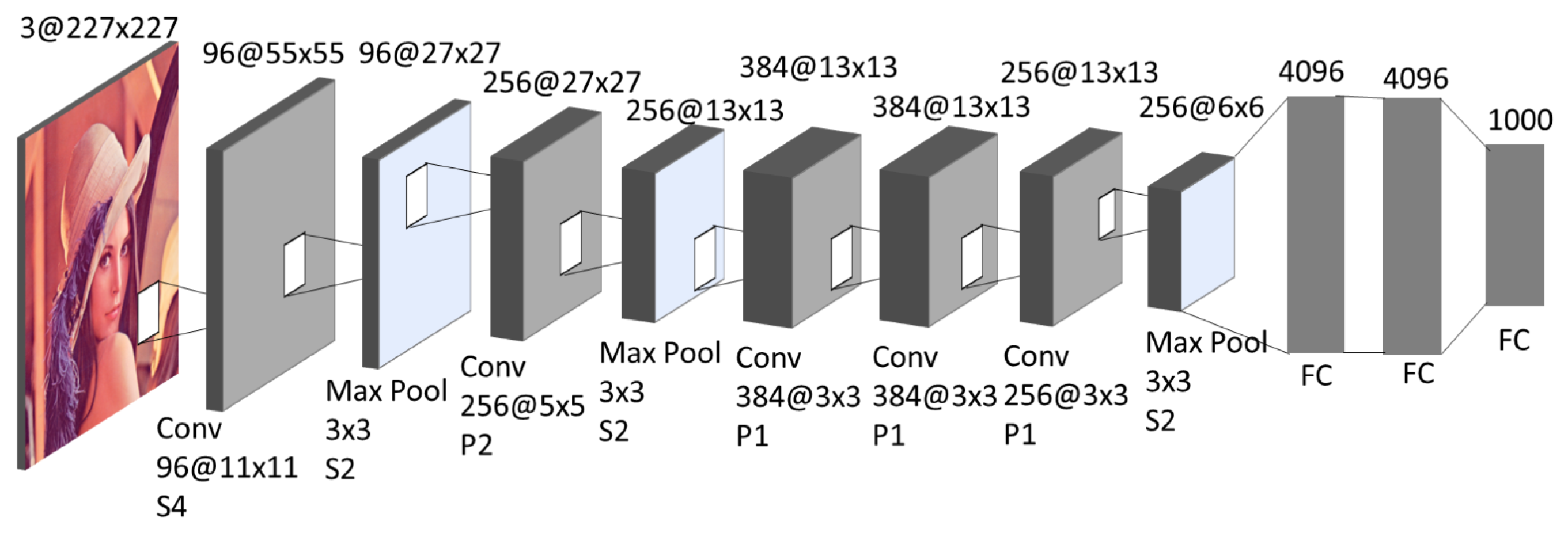
Pre-trained AlexNet [22] and VGG11 [23] models on the ILSVRC2012 dataset, as shown in Table 2, were downloaded from the PyTorch model, ZOO [24]. Both DCNN architectures, illustrated in Figure 1 and Figure 2, respectively, are purely feedforward in nature, where each layer’s input solely relies on the output of the preceding layer. AlexNet is composed of 5 convolutional layers (Conv1 to Conv5) that produce feature maps using linear spatial filters, along with 3 fully connected layers (FC1 to FC3). Following each convolutional and fully connected layer, a rectifying nonlinear unit (ReLU) of the form max (x,0) is applied to all units.
In specific convolutional layers, ReLU is followed by a subsequent max pooling sub-layer. VGG11 shares architectural similarities with AlexNet but differs in two aspects. Firstly, VGG11 employs smaller receptive fields (3 by 3 with a stride of 1) compared to AlexNet’s (11 by 11 with a stride of 4). Secondly, VGG11 possesses more layers, specifically 8 convolutional layers, compared to AlexNet.
The designation “Conv#” signifies the results of the ReLU sublayer within the convolutional layer numbered #, whereas “FC#” represents the outcomes of the #th fully connected layer following ReLU activation. To extract DCNN activations, the DNNBrain toolbox [25] was utilized. The activation map for every unit or channel was averaged to yield per-unit or per-channel activations for each instance. The activation of a unit for a specific object category was determined by averaging the per-unit responses across all instances belonging to that category.
2.3. Population Sparseness Index
The PSI value was computed for every layer of DCNNs to measure the highest point of the distribution of population responses evoked by an object category. This value corresponds to the proportion of units within the population that engaged in encoding objects, assuming binary responses [26].
where ru is the unit-wise activation of a unit u from a target layer in response to an object category, and Nu is the number of units in that layer. Activation on a unit-by-unit basis was z-scored for each unit across all categories. Subsequently, normalization was performed to scale these values from 0 to 1 across all units, thereby converting negative values into non-negative values as per the PSI’s specification. PSI values nearing 0 suggest low sparsity, signifying uniform responses across all units for the given object category. Conversely, values nearing 1 indicate high sparsity, implying that only a limited number of units respond to the category.
2.4. Adversarial Attacks
2.4.1. FGSM Attack
Szegedy et al. [27] introduced the most straightforward and rapid approach for generating adversarial examples. In order to diminish classification certainty and amplify the ambiguity between categories, fast gradient sign method (FGSM) attack involves introducing perturbations and linearizing the loss function in the direction of the gradient by (2) [27]:
where represents an adversarial example from the given input , is a randomly selected initial hyper-parameter, sign(·) is a signum function, y denotes the ground-truth label corresponding to , and represents the cost function used for training the neural network model. Additionally, (·) signifies the gradient with respect to x. FGSM attack employs analytical computations to calculate the gradient, whereas L-BFGS attack utilizes numerical optimization. As a result, FGSM attack arrives at a solution more swiftly. However, due to , FGSM attack is unable to generate a perceptual minimal difference between x and x’, unlike L-BFGS attack. Once a suitable ε value is determined through empirical means, the creation of an imperceptible adversarial sample can be achieved by applying values in its proximity.
2.4.2. PGD Attack
Projective gradient descent (PGD) attack was first introduced by Madry et al. [28]. It is an iterative version of the one-step FGSM attack. PGD can be initialized by randomly using any point within the distance of the norm of a benign sample. Each time a small step is taken, and each iteration will project the perturbation into a specified range. In a non-targeted setting, it gives an iterative formulation to craft [28]:
where Proj denotes the function to project its argument to the surface of x′s -neighbor ball. The step size is usually set to be relatively small (e.g., 1 unit of pixel change for each pixel), and step numbers guarantee that the perturbation can reach the border. This PGD attack heuristically searches the samples which have the largest loss value in the -ball around the original sample . Compared to the one-step FGSM attack algorithm, PGD attack has more flexibility, so it also has a greater adversarial attack effect.
2.4.3. CW Attack
Carlini and Wagner proposed a set of optimization-based adversarial attacks (CW attacks) that can generate and norm-measured adversarial attacks [29]. The authors employed a loss function chosen through empirical methods to induce the maximum misclassification in each norm-based attack, as in (4) [29].
where denotes the i-class’s logit, t signifies the target label, and is a parameter that embodies the minimum desired confidence margin for the adversarial examples. The loss function in (4) seeks to minimize the distance in logit values between class t and the next most similar class. When t holds the highest logit value, the disparity between the logits becomes negative, leading to optimization cessation when this logit disparity between t and the second class surpasses .
The authors demonstrated that CW attacks exhibited impressive success rates compared to contemporary attacks when assessed on the ImageNet dataset. Specifically, and -CW attacks outperformed JSMA, DeepFool attack, and FGSM attack, respectively.
3. Experimental Results
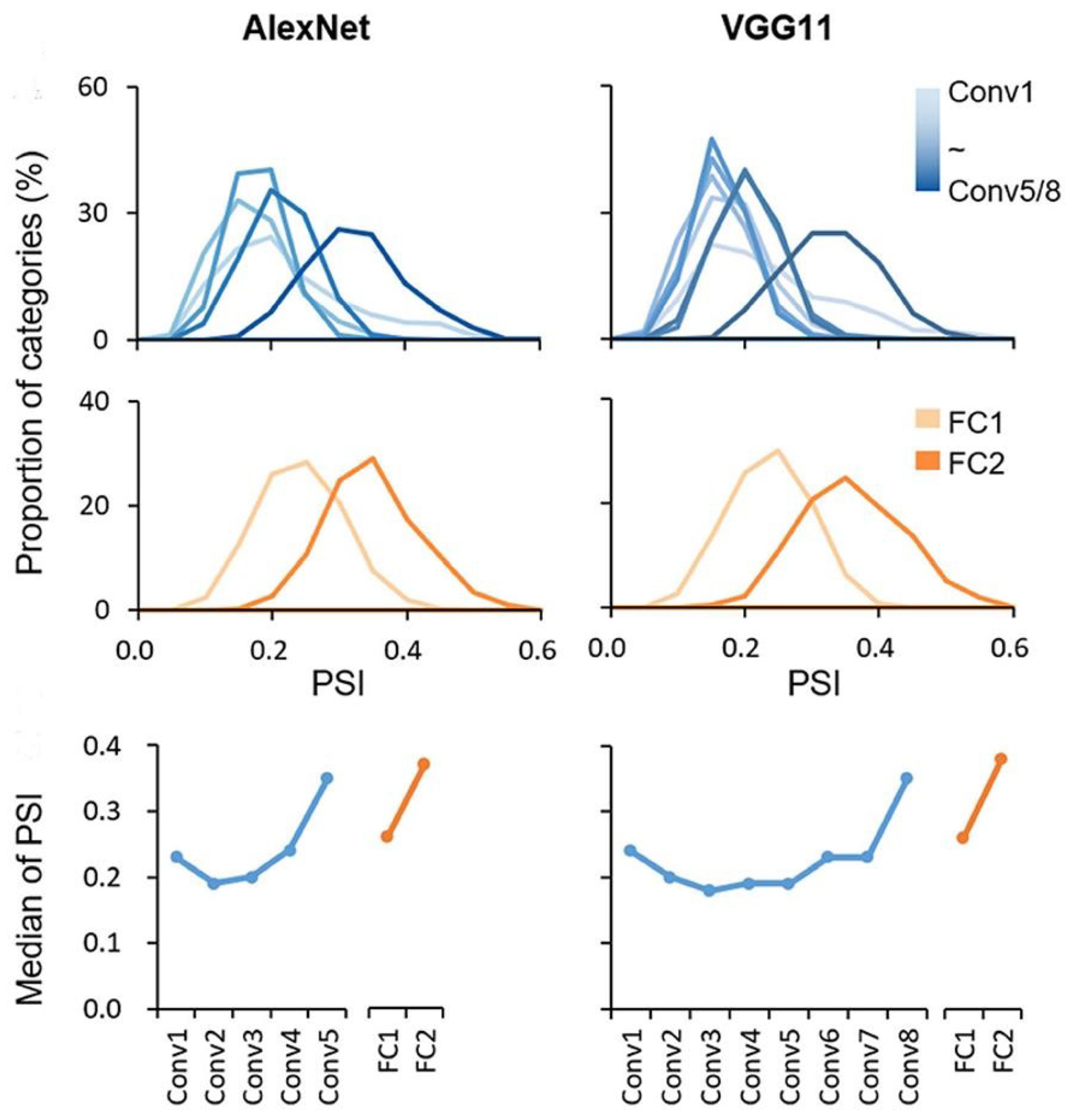
To clarify the relationship between adversarial examples and the PSI, we analyzed the research contents related to the sparseness coding scheme studied by Xingyu Liu et al. [16]. They presented significant insight regarding the PSI through the utilization of pre-trained AlexNet and VGG11 models on both the ImageNet and Caltech256 datasets. Their examination of the PSI values within the context of the ImageNet validation dataset revealed consistently modest values across all layers for every object category (median < 0.4), with the highest values not surpassing 0.6 in their conducted experiments. This observation suggests the widespread adoption of a sparse coding approach throughout all layers of the DCNNs for the purpose of object representation. Figure 3 illustrates the experimental findings depicting variations in the PSI values based on the layer, as depicted in [16].
Another noteworthy finding surfaced as the distributions of PSI for all categories exhibited considerable breadth (range > 0.2) across each layer, indicating pronounced variations in sparsity across distinct object categories. Notably, it was observed that the median PSI values displayed an inclination to rise progressively along the hierarchy, both in the convolutional and fully connected layers, respectively. The median PSI trajectory, however, was not strictly monotonic, with the initial layer showing slightly higher PSI than its immediate neighbors. Interestingly, despite the dissimilar number of convolutional layers between AlexNet and VGG11, a marked elevation in the median PSI was evident in the last two layers.
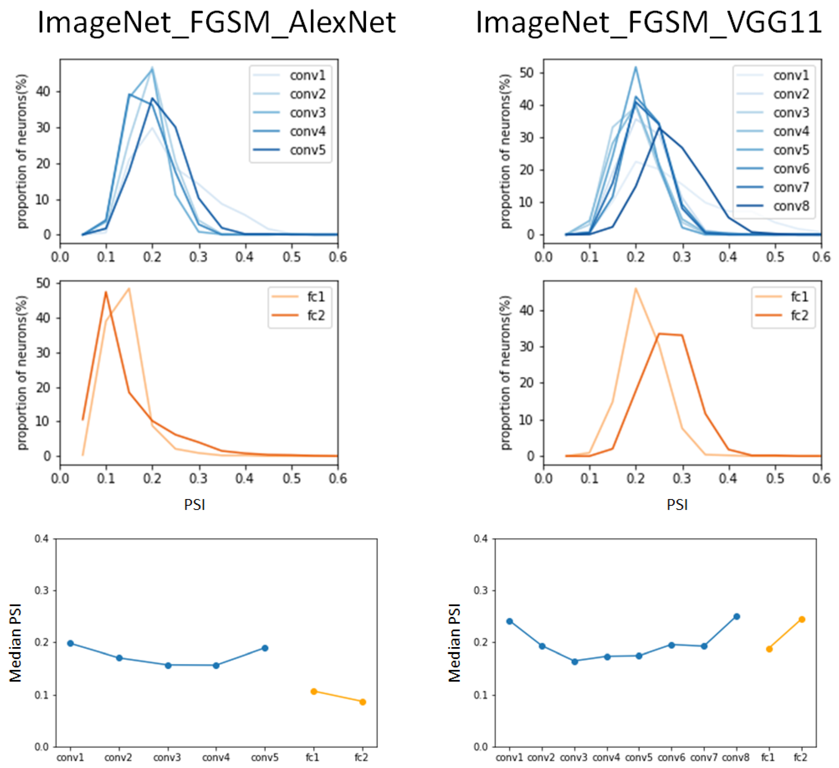
To investigate the relationship between adversarial examples and the PSI, we generated adversarial examples through FGSM attack on the ImageNet validation dataset. Then, the adversarial examples by FGSM attack were applied to pre-trained AlexNet and VGG11 models. Figure 4 shows the hierarchical sparse coding for object categories by FGSM-attacked adversarial examples in AlexNet and VGG11.
It was commonly observed in AlexNet and VGG11 that the median of the PSI in the FGSM-attacked ImageNet dataset was in a lower range (median < 2.5) than the values in the benign ImageNet dataset. In the experimental results in [16], the median of the PSI in AlexNet gradually increased after convolutional layer 2, but in the case of FGSM attack, it continuously decreased until convolutional layer 4, and then increased in the last convolutional layer. In the fully connected layer, the value of the median of the PSI rather decreased, which is opposite to the result in [16].
In comparison to the normal validation ImageNet dataset in Figure 3, despite the increase in the number of layers in AlexNet, the graph hardly shifted to the right; rather, a left shift was observed in the fully connected layer. From the overall observation, the change in the PSI due to FGSM attack shows that the value of the median of the PSI was lower compared to the normal case, and a right shift of the graph rarely occurred.
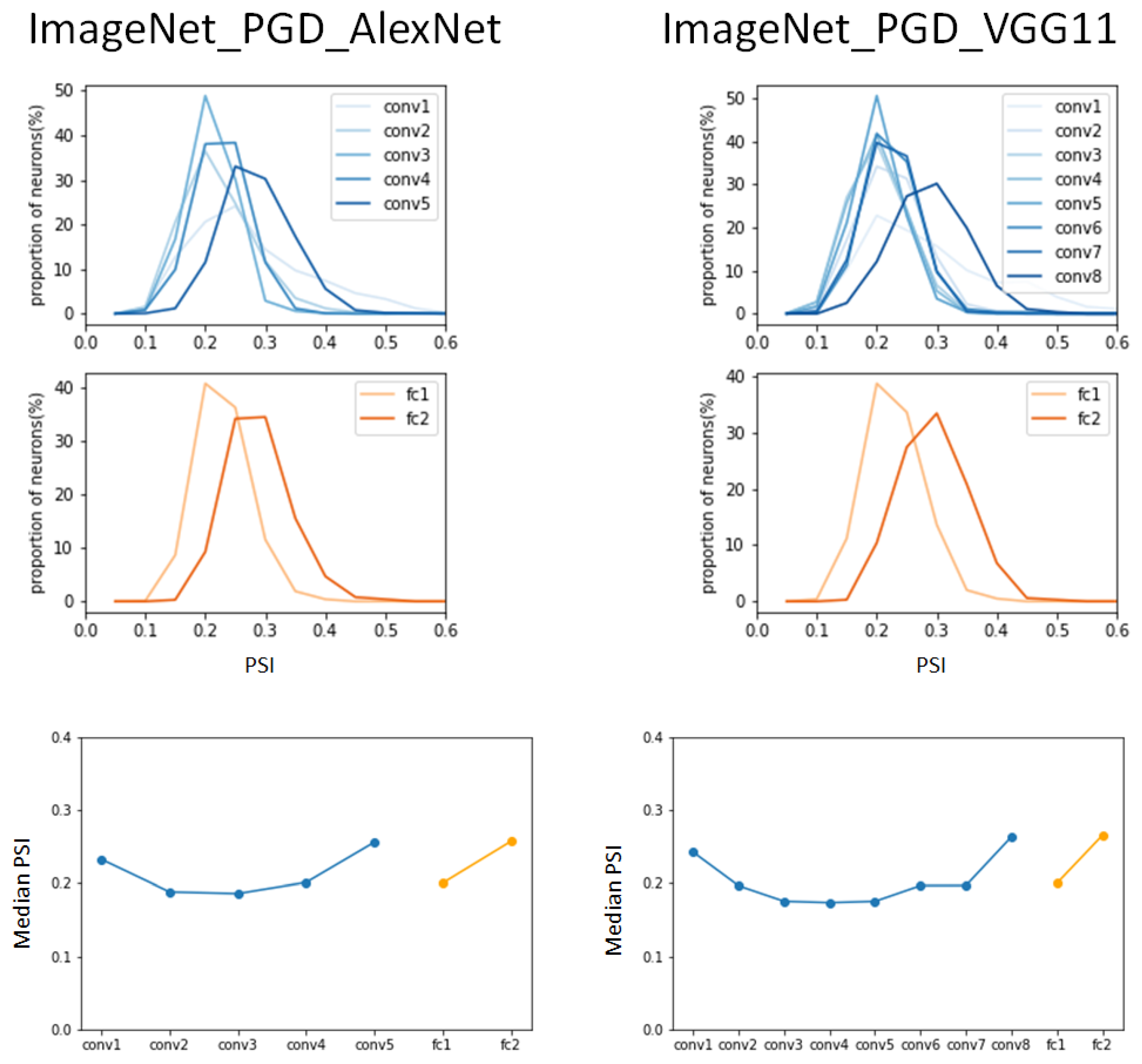
The same experiment was performed on the pre-trained AlexNet and VGG11 on adversarial examples of ImageNet attacked by PGD attack. The result of the median of the PSI was less than 0.3, which is smaller than the result from the non-attacked ImageNet validation dataset (typical dataset) shown in Figure 5. Although the median value of the PSI in the first convolutional layer was observed to be similar to that in the typical ImageNet dataset, there was no rapid increase in the median PSI values as the hierarchy progressed. The range of change in the median PSI values at the convolution layers was 0.18 to 0.35 for the typical ImageNet dataset, 0.15 to 0.20 for the ImageNet dataset attacked by FGSM attack, and 0.19 to 0.26 for the ImageNet dataset attacked by PGD attack.
The right shifting in the convolutional layers and fully connected layers according to the hierarchy was more pronounced than in the FGSM attack. However, it did not reach the results of the typical ImageNet dataset. In the graph of the PSI versus the proportion of categories, the PGD-attacked ImageNet dataset shows a right shift, with the peak values of the PSI in the range of 0.2 to 0.3 in Figure 5, while the FGSM-attacked ImageNet dataset had a right shift from 0.12 to 0.4 in Figure 4, and the typical ImageNet dataset had a right shift from 0.1 to 0.25 in Figure 3.
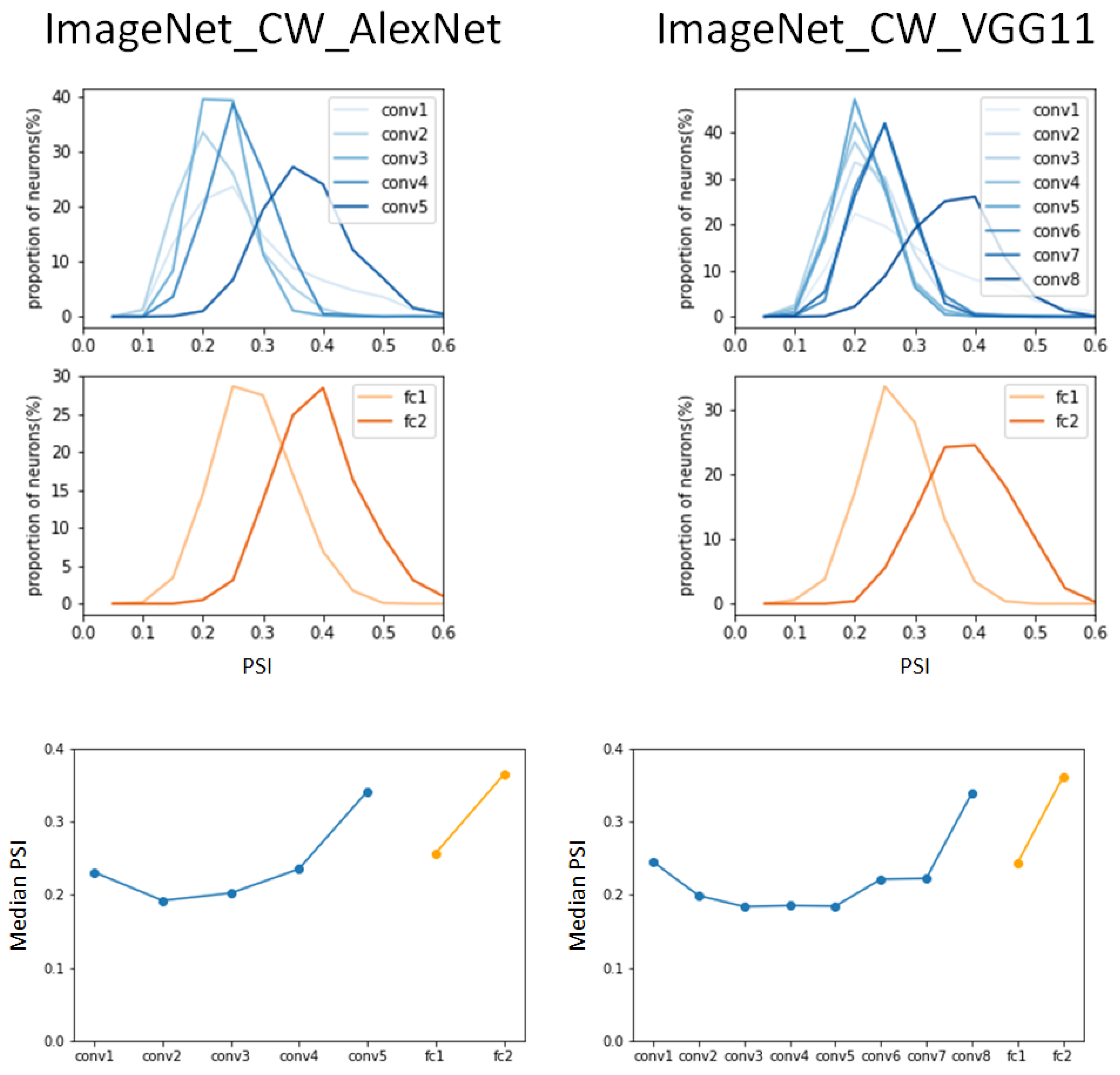
The final experiment for the hierarchical sparse coding for object categories using the ImageNet dataset was performed on the same DCNNs using the CW-attacked ImageNet dataset. The experiments with the CW-attacked ImageNet dataset had interesting results in contrast to the results of the previously described FGSM attack and PGD attack. The CW attack results in Figure 6 are very similar to the results in Figure 3. The range of median PSI values from 0.19 to 0.35 is very similar to the range from 0.18 to 0.38 as a result of applying the typical ImageNet dataset, and the pattern of change in the PSI according to the hierarchy is also very similar.
In the PSI versus the proportion of categories graph, the pattern of shifts to the right is such that the peaks of the PSI distribution move from 0.2 to 0.4 for AlexNet and VGG11, while for the typical ImageNet datasets, they move from 0.12 to 0.4 for AlexNet and from 0.2 to move 0.4 for VGG11.
Comparing the three attack methods, namely FGSM Attack, PGD attack, and CW attack, in terms of attack strength, CW attack is the strongest attack method and PGD Attack is the second strongest attack method based on FGSM attack [30]. From the results of the four experiments in Figure 6, it can be deduced that the stronger the attack and the more difficult it is to defend against it, the more difficult it is to distinguish the hierarchical sparseness from the hierarchical sparseness of the DCNN trained with a typical dataset.
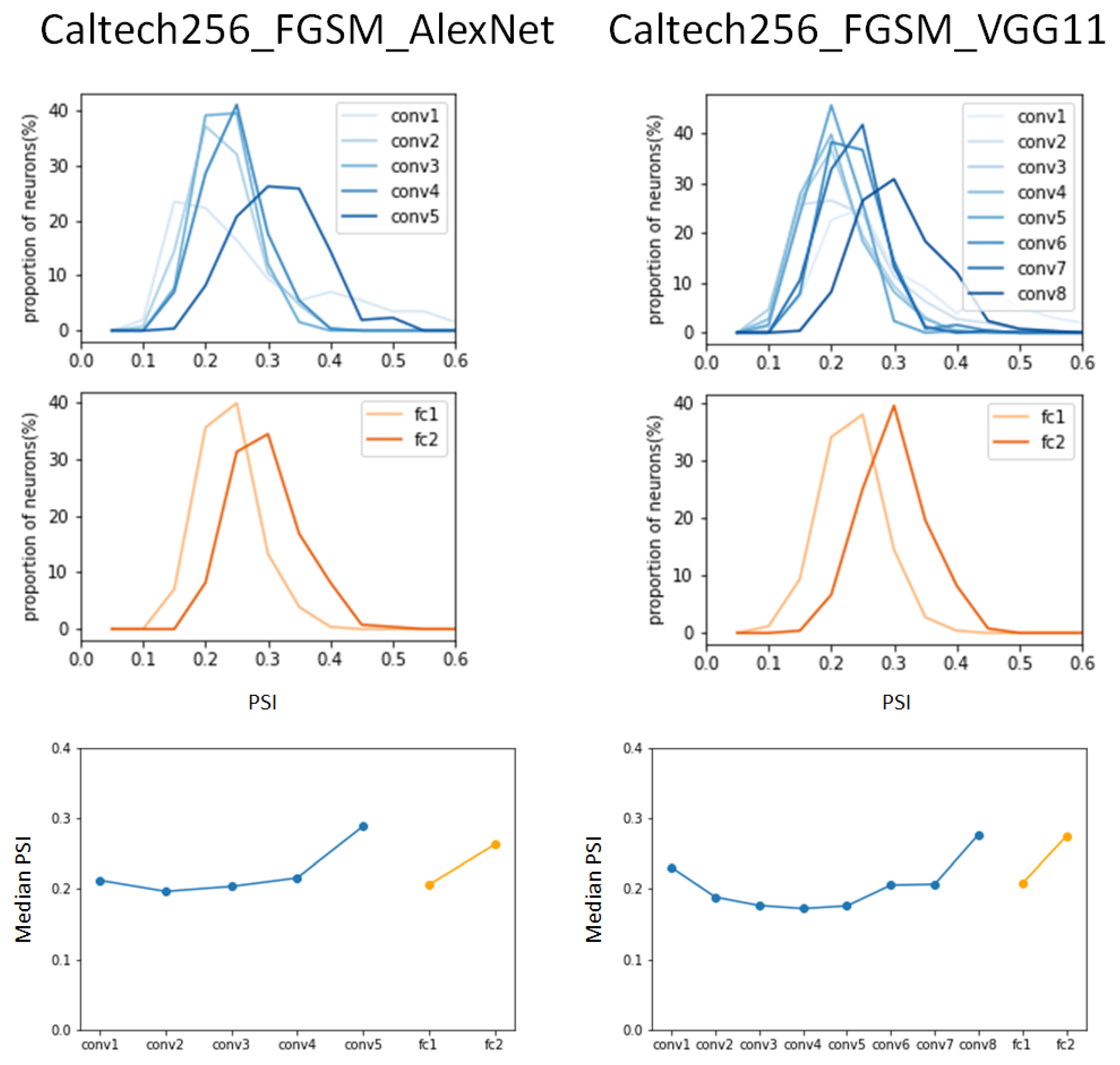
We conducted the same experiment to observe whether the same results were obtained when different datasets were applied to the same DCNN models. That is, the same experiment was carried out by applying the Caltech256 dataset to the VGG11 and the AlexNet models. Figure 7 shows the PSI results of the VGG11 and AlexNet models for the FGSM-attacked Caltech256 dataset.
When comparing the changes in the peak values of the PSI distribution by layer in the AlexNet model, it can be observed that the FGSM-attacked dataset shows lower peak values compared to the results of the benign Caltech256 dataset. In addition, it can be seen that in the fully connected layers, significant low values are indicated. That is, the peak values of the benign Caltech256 dataset were 0.27 and 0.42 in fully connected layer 1 and fully connected layer 2, but 0.18 and 0.19 in the FGSM-attacked Caltect256 dataset.
The same results were observed in the VGG11 model. A decrease in the peak values in the PSI distribution was observed overall, and a peak value reduction of up to 50% was observed in the fully connected layers. In the median PSI comparison, the convolution layers show a pattern similar to the results of the benign Caltec256 dataset, but an increase was observed in the fully connected layers.
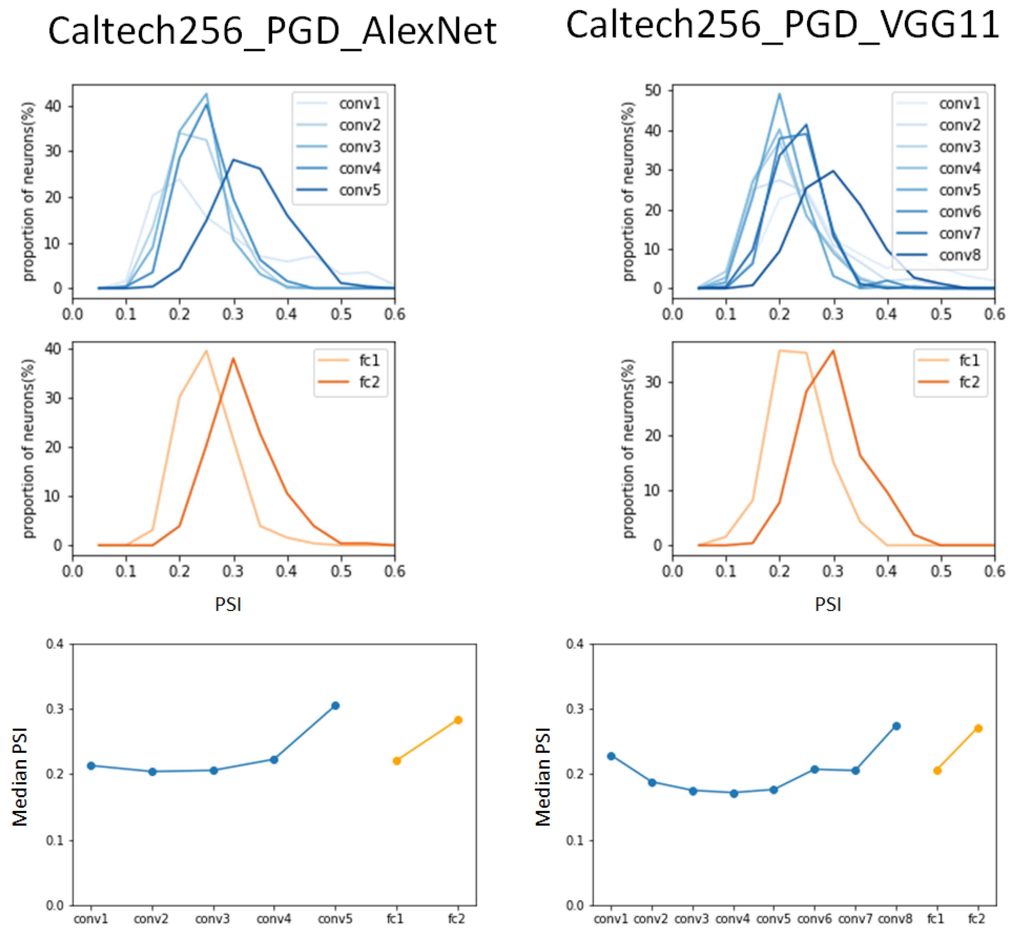
In the same experiment on the PGD-attacked Caltech356 dataset, the AlexNet model was observed to exhibit higher peak values in the PSI distribution compared to the results of the ImageNet dataset that was subjected to the same attack in Figure 8. It is worth noting that in the PGD-attacked ImageNet dataset, the peak value of the PSI decreased as it progressed from fully connected layer 1 to fully connected layer 2, but in the PGD-attacked Caltech256 dataset, it increased, as it did in both benign datasets. The VGG11 model shows very similar results to the benign Caltech256 dataset in the convolution layers, but it was observed that the peak value of the PSI distribution decreased sharply in fully connected layer 1 and then recovered to a value similar to that of the benign dataset in fully connected layer 2.
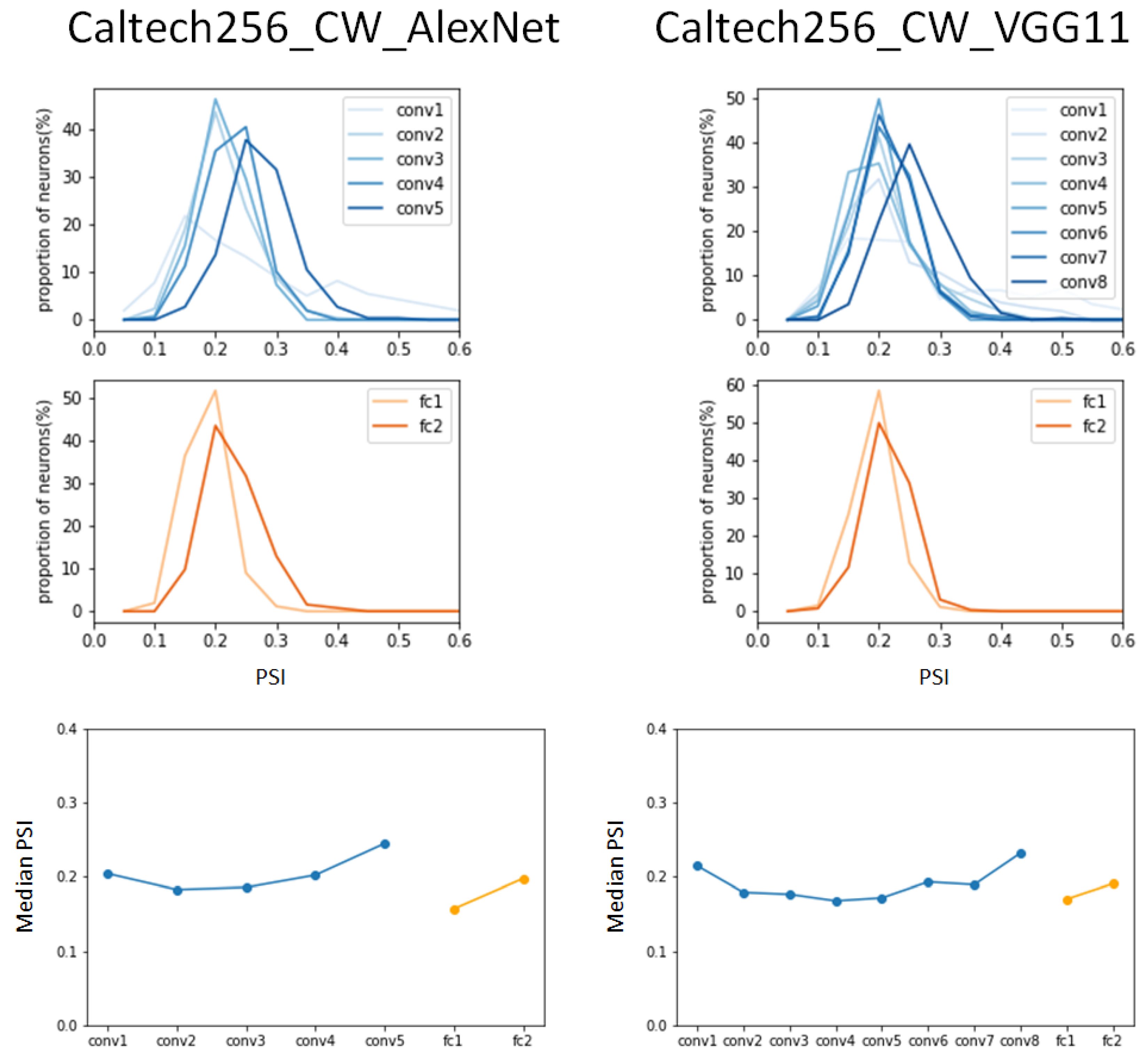
In the experiments with the CW-attacked Catech256 dataset, the AlexNet model had peak values that were similar to or slightly lower than those of the benign Caltech256 dataset in the convolution layers in Figure 9. A slightly lower value was observed in fully connected layer 1 compared to the results of the benign dataset, but a peak value of 0.28 was observed in fully connected layer 2, which was significantly smaller than the peak value of 0.42 in the benign dataset.
In addition, the VGG11 model showed almost the same experimental results as the benign Caltech256 dataset, although convolution layer 6 showed a different peak value. In the analysis of the median PSI, it was observed that the results of the AlexNet model were almost identical to the results of the benign Caltech256 dataset, and a pattern similar to the results of the AlexNet model was found in the VGG11 model. This study involved analyzing the coding scheme across various layers of two conventional DCNNs, AlexNet and VGG11, using two attacked versions of datasets—ImageNet and Caltech256.
The results of our experiments can be summarized as shown in Table 3 and Table 4 for the median PSI analysis and in Table 5 and Table 6 for the PSI peak value analysis. These tables present the layer-specific median PSI values and PSI peak values, offering insights into the level of sparsity within each layer of conventional DCNNs, AlexNet and VGG11.
In the PSI analysis of the two DCNN models for the benign examples, it was found that the PSI, as the degree of sparseness, increased with the increase in the layers in the DCNNs. The observation that an increased median PSI at each layer aligned with greater behavioral relevance within the DCNNs implies that this phenomenon serves as a fundamental mechanism for efficiently representing a diverse range of objects.
Essentially, this suggests that in the initial stages of visual processing, a larger population of general neurons is engaged to accurately process various natural objects. As we move up the processing hierarchy, these objects are parsed into more abstract features, leading to the involvement of a smaller, yet highly specialized, group of neurons in constructing this representation. This heightened level of sparsity significantly enhances the interpretability of these representations, as the extent of sparsity appears to predict behavioral performance primarily in the higher processing stages [16].
As shown in the median PSI values for the benign examples of the AlexNet and VGG11 models in Table 3, the median PSI values tended to increase progressively from convolution layer 2 to convolution layer 5 in AlexNet and to convolution layer 8 in VGG11, except for convolution layer 1. In the case of the Caltech256 dataset in Table 4, when benign examples were applied to the two models, it can be observed that the median PSI increased along the convolution layers entirely.
In addition, as shown in the study of [16], it was observed that the last convolution layer, which corresponds to conv5 in AlexNet and conv8 in VGG11, and the last fully connected layers in the two models had a dramatical decrease in the median PSI value.
In the PSI analysis, the same tendency was observed in the adversarial examples in both DCNN model. In particular, we found that in the adversarial examples generated from FGSM and PGD attack, not only did the median PSI increase slowly according to the layer, but it also showed a lower median PSI value compared to the results of the benign examples. Interestingly, the change in the median PSI was observed to show a rate of change of 1.0–1.3 for the benign examples from fc1 to fc2, while a rate of change of 0–0.8 during the same transition layer for both attacks. These results are interpreted as affecting the behavioral performance of DCNN models since specialized groups of neurons do not work when adversarial examples are applied to DCNN models. Note that the changes in sparseness were observed in two structurally similar DCNNs in AlexNet and VGG11, and therefore, this may not be applicable to other DCNNs.
We found interesting results related to the median PSI from CW-attacked datasets. The median PSI for each layer for the CW adversarial examples generated from the ImageNet dataset, as shown in Table 3, showed values that are almost similar to the results of the benign examples in the AlexNet and VGG11 models. Although the median PSI at fc2 was slightly smaller than the results of the benign examples, the median PSI for the entire layer was similar. The same results were also obtained in the CW-adversarial examples obtained from the Caltech256 dataset.
4. Conclusions
This study represents the coding scheme of adversarial examples generated from three adversarial attacks and provides information on how adversarial examples behave inside DCNNs. In particular, we observed that the AlexNet and VGG11 models, which have similar but different structures, exhibited similar PSI characteristics for the adversarial examples generated from each attack, and confirmed that the DCNNs behaved abnormally. A notable observation is that the median PSI values at the final fully connected layer of the two DCNN models, which ultimately determine the models’ performance, were lower when compared to the PSI values of the benign examples. This phenomenon was more pronounced in the attacked ImageNet dataset. These results suggest a perturbation in the features of samples caused by adversarial examples.
Our research can be considered from the perspective of DCNN model design and from a neurophysiological perspective. The first aspect provides a basis for revealing the internal mechanisms of DCNNs that cause malfunctions by adversarial examples. Consequently, considering the internal dynamics of DCNN models known as black boxes, it can be applied to design more robust DCNN models against adversarial attacks.
From a neurophysiological point of view, it provides a macro- and micro-perspective on how we misperceive objects. In other words, brain studies targeting non-human primates have limited spatial resolution or brain area, but DCNNs can clearly observe the activity of neuron units, so it is possible to conduct research without such limitations.
Therefore, although our study was limited to two types of DCNN models and three types of adversarial examples from two datasets, it is valuable as a new attempt to understand adversarial attacks in DCNN structures. Beyond the constraints of the models and datasets used in this experiment, investigating the internal dynamics of models using PSI for other models and datasets remains a future research task.
Author Contributions
Conceptualization, Y.L. and J.K.; methodology, Y.L. and J.K.; software, Y.L. and J.K.; validation, Y.L. and J.K.; formal analysis, Y.L. and J.K.; investigation, Y.L. and J.K.; resources, Y.L. and J.K.; data curation, Y.L.; writing—original draft preparation, Y.L. and J.K.; writing—review and editing, Y.L. and J.K.; visualization, Y.L. and J.K.; supervision, Y.L. and J.K.; project administration, Y.L. and J.K.; funding acquisition, Y.L. and J.K. All authors have read and agreed to the published version of the manuscript.
Funding
This work was conducted with the support of the National Research Foundation of Korea (NRF-2020RIA2C1101938).
Institutional Review Board Statement
Not Applicable.
Informed Consent Statement
Not Applicable.
Data Availability Statement
Not Applicable.
Conflicts of Interest
The authors declare no conflict of interest.
References
- Sharma, N.; Jain, V.; Mishra, A. An Analysis Of Convolutional Neural Networks For Image Classification. Procedia Comput. Sci. 2018, 132, 377–384. [Google Scholar] [CrossRef]
- Wang, W.; Yang, Y.; Wang, X.; Wang, W.; Li, J. Development of convolutional neural network and its application in image classification: A survey. Opt. Eng. 2019, 58, 040901. [Google Scholar] [CrossRef]
- Maurer, D.; Lewis, T.L. Chapter 8—Visual Systems. In The Neurobiology of Brain and Behavioral Development; Gibb, R., Kolb, B., Eds.; Academic Press: Cambridge, MA, USA, 2018; pp. 213–233. ISBN 978-0-12-804036-2. [Google Scholar]
- Goodfellow, I.J.; Shlens, J.; Szegedy, C. Explaining and Harnessing Adversarial Examples. arXiv 2015, arXiv:1412.6572. [Google Scholar]
- Philipp, G.; Carbonell, J.G. The Nonlinearity Coefficient—Predicting Generalization in Deep Neural Networks. arXiv 2019, arXiv:1806.00179. [Google Scholar]
- Li, T.; Wang, F.; Zhou, Y.; Xie, Z. Visual illusion cognition dataset construction and recognition performance by deep neural networks. In Proceedings of the 2022 IEEE 8th International Conference on Cloud Computing and Intelligent Systems (CCIS), Chengdu, China, 26–28 November 2022; pp. 90–94. [Google Scholar]
- Failor, S.W.; Carandini, M.; Harris, K.D. Learning orthogonalizes visual cortical population codes. bioRxiv 2021. [Google Scholar] [CrossRef]
- Wang, J. Adversarial Examples in Physical World. In Proceedings of the Thirtieth International Joint Conference on Artificial Intelligence, Montreal. QC, Canada, 19–27 August 2021; pp. 4925–4926. [Google Scholar]
- Chakraborty, A.; Alam, M.; Dey, V.; Chattopadhyay, A.; Mukhopadhyay, D. A survey on adversarial attacks and defenses—Chakraborty. CAAI Trans. Intell. Technol. 2021, 6, 25–45. [Google Scholar] [CrossRef]
- Akhtar, N.; Mian, A.; Kardan, N.; Shah, M. Advances in Adversarial Attacks and Defenses in Computer Vision: A Survey. IEEE Access 2021, 9, 155161–155196. [Google Scholar] [CrossRef]
- Xu, H.; Ma, Y.; Liu, H.-C.; Deb, D.; Liu, H.; Tang, J.-L.; Jain, A.K. Adversarial Attacks and Defenses in Images, Graphs and Text: A Review. Int. J. Autom. Comput. 2020, 17, 151–178. [Google Scholar] [CrossRef]
- Benz, P.; Ham, S.; Zhang, C.; Karjauv, A.; Kweon, I.S. Adversarial Robustness Comparison of Vision Transformer and MLP-Mixer to CNNs. arXiv 2021. [Google Scholar] [CrossRef]
- Buhrmester, V.; Münch, D.; Arens, M. Analysis of Explainers of Black Box Deep Neural Networks for Computer Vision: A Survey. Mach. Learn. Knowl. Extr. 2021, 3, 966–989. [Google Scholar] [CrossRef]
- Rudin, C. Stop explaining black box machine learning models for high stakes decisions and use interpretable models instead. Nat. Mach. Intell. 2019, 1, 206–215. [Google Scholar] [CrossRef]
- Loyola-González, O. Black-Box vs. White-Box: Understanding Their Advantages and Weaknesses from a Practical Point of View. IEEE Access 2019, 7, 154096–154113. [Google Scholar] [CrossRef]
- Liu, X.; Zhen, Z.; Liu, J. Hierarchical Sparse Coding of Objects in Deep Convolutional Neural Networks. Front. Comput. Neurosci. 2020, 14, 578158. [Google Scholar] [CrossRef] [PubMed]
- Quiroga, R.Q.; Kreiman, G. Measuring sparseness in the brain: Comment on. Psychol. Rev. 2010, 117, 291–297. [Google Scholar] [CrossRef] [PubMed]
- Luo, W.; Liu, W.; Lian, D.; Tang, J.; Duan, L.; Peng, X.; Gao, S. Video Anomaly Detection with Sparse Coding Inspired Deep Neural Networks. IEEE Trans. Pattern Anal. Mach. Intell. 2021, 43, 1070–1084. [Google Scholar] [CrossRef]
- Alzubaidi, L.; Zhang, J.; Humaidi, A.J.; Al-Dujaili, A.; Duan, Y.; Al-Shamma, O.; Santamaría, J.; Fadhel, M.A.; Al-Amidie, M.; Farhan, L. Review of deep learning: Concepts, CNN architectures, challenges, applications, future directions. J. Big Data 2021, 8, 53. [Google Scholar] [CrossRef]
- Russakovsky, O.; Deng, J.; Su, H.; Krause, J.; Satheesh, S.; Ma, S.; Huang, Z.; Karpathy, A.; Khosla, A.; Bernstein, M.; et al. ImageNet Large Scale Visual Recognition Challenge. Int. J. Comput. Vis. 2015, 115, 211–252. [Google Scholar] [CrossRef]
- Griffin, G.; Holub, A.; Perona, P. Caltech-256 Object Category Dataset; California Institute of Technology: Pasadena, CA, USA, 2007. [Google Scholar]
- Krizhevsky, A.; Sutskever, I.; Hinton, G.E. ImageNet Classification with Deep Convolutional Neural Networks. In Advances in Neural Information Processing Systems; Curran Associates, Inc.: Red Hook, NY, USA, 2012; Volume 25. [Google Scholar]
- Simonyan, K.; Zisserman, A. Very Deep Convolutional Networks for Large-Scale Image Recognition. arXiv 2015, arXiv:1409.1556. [Google Scholar]
- PyTorch. Model Zoo—Serve Master Documentation. Available online: https://pytorch.org/serve/model_zoo.html (accessed on 4 June 2023).
- Chen, X.; Zhou, M.; Gong, Z.; Xu, W.; Liu, X.; Taicheng, H.; Zhen, Z.; Liu, J. DNNBrain: A Unifying Toolbox for Mapping Deep Neural Networks and Brains. Front. Comput. Neurosci. 2020, 14, 580632. [Google Scholar] [CrossRef]
- Vinje, W.E.; Gallant, J.L. Sparse coding and decorrelation in primary visual cortex during natural vision. Science 2000, 287, 1273–1276. [Google Scholar] [CrossRef]
- Szegedy, C.; Zaremba, W.; Sutskever, I.; Bruna, J.; Erhan, D.; Goodfellow, I.; Fergus, R. Intriguing properties of neural networks. arXiv 2014, arXiv:1312.6199. [Google Scholar]
- Madry, A.; Makelov, A.; Schmidt, L.; Tsipras, D.; Vladu, A. Towards Deep Learning Models Resistant to Adversarial Attacks. arXiv 2019, arXiv:1706.06083. [Google Scholar]
- Carlini, N.; Wagner, D. Towards Evaluating the Robustness of Neural Networks. In Proceedings of the 2017 IEEE Symposium on Security and Privacy (SP), San Jose, CA, USA, 22–26 May 2017. [Google Scholar]
- Li, Y.; Cheng, M.; Hsieh, C.-J.; Lee, T.C.M. A Review of Adversarial Attack and Defense for Classification Methods. Am. Stat. 2022, 76, 329–345. [Google Scholar] [CrossRef]
Figure 1.
AlexNet architecture.

Figure 2.
VGG11 architecture.

Figure 3.
Experimental results in [16] of hierarchical sparse coding for object categories in DCNNs. The sparsity was assessed by means of the PSI for individual object categories within each layer, employing the ImageNet dataset.
Figure 3.
Experimental results in [16] of hierarchical sparse coding for object categories in DCNNs. The sparsity was assessed by means of the PSI for individual object categories within each layer, employing the ImageNet dataset.

Figure 4.
Hierarchical sparse coding for object categories by FGSM adversarial samples in DCNN. In comparison to the results of the normal ImageNet validation dataset in Figure 3, the right shift of the graph hardly occurs despite the increase in the number of layers in AlexNet.
Figure 4.
Hierarchical sparse coding for object categories by FGSM adversarial samples in DCNN. In comparison to the results of the normal ImageNet validation dataset in Figure 3, the right shift of the graph hardly occurs despite the increase in the number of layers in AlexNet.

Figure 5.
Hierarchical sparse coding for object categories by PGD adversarial samples in DCNN. In comparison with the result of FGSM attack, the similarity is that the median of the PSI is in a low range, and the difference is that a slight right shift occurs.
Figure 5.
Hierarchical sparse coding for object categories by PGD adversarial samples in DCNN. In comparison with the result of FGSM attack, the similarity is that the median of the PSI is in a low range, and the difference is that a slight right shift occurs.

Figure 6.
Hierarchical sparse coding for object categories by CW adversarial samples in DCNN.

Figure 7.
PSI results of VGG11 and AlexNet models by FGSM-attacked Caltech256 dataset.

Figure 8.
PSI results of VGG11 and AlexNet models by PGD-attacked Caltech256 dataset.

Figure 9.
PSI results of VGG11 and AlexNet models by CW-attacked Caltech256 dataset.


Table 1.
Specifications of ImageNet and Caltech256 datasets.
| Dataset | Training | Validation | Testing | Categories | |||
|---|---|---|---|---|---|---|---|
| ImageNet | 1,281,167 | 50,000 | 100,000 | 1000 | |||
| Caltech256 | Total data | Data/Category | Categories | ||||
| 30,607 | Min. | Med. | Avg. | Max. | 256 | ||
| 80 | 100 | 119 | 827 | ||||
Table 2.
Configurations of VGG11 and AlexNet architectures.
| Layer | No. of Layer | VGG11 | AlexNet |
|---|---|---|---|
| Convolution layer | 1 | Conv3-64 | Conv11-96 |
| 2 | Conv3-128 | Conv5-256 | |
| 3 | Conv3-256 | Conv-3-384 | |
| 4 | Conv-3-256 | Conv-3-384 | |
| 5 | Conv-3-512 | Conv-3-256 | |
| 6 | Conv-3-512 | ||
| 7 | Conv-3-512 | ||
| 8 | Conv-3-512 | ||
| FC layer | 1 | FC-4096 | FC-4096 |
| 2 | FC-4096 | FC-4096 | |
| Output layer | FC-1000 | FC-1000 |
Table 3.
Layer-wise median PSIs in AlexNet and VGG11 models for benign and adversarial examples from attacked ImageNet datasets.
Table 3.
Layer-wise median PSIs in AlexNet and VGG11 models for benign and adversarial examples from attacked ImageNet datasets.
| Model | Layer | Median PSI Value | |||
|---|---|---|---|---|---|
| Benign | FGSM | PGD | CW | ||
| AlexNet | conv1 | 0.23 | 0.20 | 0.23 | 0.22 |
| conv2 | 0.18 | 0.16 | 0.19 | 0.19 | |
| conv3 | 0.19 | 0.15 | 0.19 | 0.19 | |
| conv4 | 0.25 | 0.15 | 0.21 | 0.20 | |
| conv5 | 0.35 | 0.18 | 0.26 | 0.35 | |
| fc1 | 0.27 | 0.12 | 0.18 | 0.25 | |
| fc2 | 0.37 | 0.08 | 0.22 | 0.36 | |
| VGG11 | conv1 | 0.24 | 0.24 | 0.24 | 0.23 |
| conv2 | 0.21 | 0.18 | 0.20 | 0.20 | |
| conv3 | 0.19 | 0.16 | 0.18 | 0.19 | |
| conv4 | 0.20 | 0.17 | 0.18 | 0.19 | |
| conv5 | 0.20 | 0.17 | 0.17 | 0.19 | |
| conv6 | 0.25 | 0.19 | 0.21 | 0.21 | |
| conv7 | 0.25 | 0.18 | 0.20 | 0.21 | |
| conv8 | 0.35 | 0.26 | 0.26 | 0.35 | |
| fc1 | 0.27 | 0.17 | 0.19 | 0.22 | |
| fc2 | 0.38 | 0.25 | 0.25 | 0.36 | |
Table 4.
Layer-wise median PSIs in AlexNet and VGG11 models for benign and adversarial examples from attacked Caltech256 datasets.
Table 4.
Layer-wise median PSIs in AlexNet and VGG11 models for benign and adversarial examples from attacked Caltech256 datasets.
| Model | Layer | Median PSI Value | |||
|---|---|---|---|---|---|
| Benign | FGSM | PGD | CW | ||
| AlexNet | conv1 | 0.20 | 0.21 | 0.21 | 0.21 |
| conv2 | 0.16 | 0.20 | 0.20 | 0.17 | |
| conv3 | 0.17 | 0.21 | 0.20 | 0.18 | |
| conv4 | 0.19 | 0.22 | 0.23 | 0.20 | |
| conv5 | 0.22 | 0.28 | 0.33 | 0.23 | |
| fc1 | 0.16 | 0.22 | 0.23 | 0.15 | |
| fc2 | 0.29 | 0.26 | 0.28 | 0.25 | |
| VGG11 | conv1 | 0.20 | 0.23 | 0.13 | 0.22 |
| conv2 | 0.19 | 0.18 | 0.17 | 0.18 | |
| conv3 | 0.19 | 0.17 | 0.18 | 0.17 | |
| conv4 | 0.18 | 0.17 | 0.17 | 0.16 | |
| conv5 | 0.18 | 0.17 | 0.18 | 0.17 | |
| conv6 | 0.20 | 0.22 | 0.19 | 0.19 | |
| conv7 | 0.20 | 0.21 | 0.19 | 0.18 | |
| conv8 | 0.25 | 0.28 | 0.24 | 0.24 | |
| fc1 | 0.16 | 0.19 | 0.17 | 0.17 | |
| fc2 | 0.29 | 0.27 | 0.17 | 0.25 | |
Table 5.
Layer-wise PSI peak values in AlexNet and VGG11 models for benign and adversarial examples from attacked ImageNet dataset.
Table 5.
Layer-wise PSI peak values in AlexNet and VGG11 models for benign and adversarial examples from attacked ImageNet dataset.
| Model | Layer | PSI Peak Value | |||
|---|---|---|---|---|---|
| Benign | FGSM | PGD | CW | ||
| AlexNet | conv1 | 0.22 | 0.20 | 0.25 | 0.24 |
| conv2 | 0.17 | 0.21 | 0.17 | 0.17 | |
| conv3 | 0.16 | 0.22 | 0.18 | 0.17 | |
| conv4 | 0.22 | 0.13 | 0.18 | 0.24 | |
| conv5 | 0.26 | 0.17 | 0.23 | 0.35 | |
| fc1 | 0.26 | 0.08 | 0.17 | 0.24 | |
| fc2 | 0.36 | 0.16 | 0.30 | 0.43 | |
| VGG11 | conv1 | 0.15 | 0.20 | 0.17 | 0.17 |
| conv2 | 0.15 | 0.19 | 0.18 | 0.18 | |
| conv3 | 0.14 | 0.18 | 0.18 | 0.18 | |
| conv4 | 0.14 | 0.18 | 0.19 | 0.19 | |
| conv5 | 0.13 | 0.17 | 0.19 | 0.20 | |
| conv6 | 0.22 | 0.16 | 0.20 | 0.20 | |
| conv7 | 0.22 | 0.16 | 0.20 | 0.33 | |
| conv8 | 0.25 | 0.24 | 0.33 | 0.36 | |
| fc1 | 0.23 | 0.20 | 0.18 | 0.13 | |
| fc2 | 0.37 | 0.23 | 0.32 | 0.32 | |
Table 6.
Layer-wise PSI peak values in AlexNet and VGG11 models for benign and adversarial examples from attacked Caltech256 dataset.
Table 6.
Layer-wise PSI peak values in AlexNet and VGG11 models for benign and adversarial examples from attacked Caltech256 dataset.
| Model | Layer | PSI Peak Value | |||
|---|---|---|---|---|---|
| Benign | FGSM | PGD | CW | ||
| AlexNet | conv1 | 0.17 | 0.14 | 0.17 | 0.13 |
| conv2 | 0.17 | 0.18 | 0.18 | 0.18 | |
| conv3 | 0.23 | 0.19 | 0.24 | 0.25 | |
| conv4 | 0.24 | 0.26 | 0.25 | 0.23 | |
| conv5 | 0.33 | 0.26 | 0.28 | 0.30 | |
| fc1 | 0.27 | 0.18 | 0.23 | 0.23 | |
| fc2 | 0.42 | 0.19 | 0.28 | 0.28 | |
| VGG11 | conv1 | 0.26 | 0.13 | 0.13 | 0.25 |
| conv2 | 0.17 | 0.17 | 0.17 | 0.13 | |
| conv3 | 0.17 | 0.18 | 0.18 | 0.16 | |
| conv4 | 0.18 | 0.17 | 0.17 | 0.17 | |
| conv5 | 0.18 | 0.18 | 0.18 | 0.18 | |
| conv6 | 0.23 | 0.19 | 0.19 | 0.19 | |
| conv7 | 0.23 | 0.19 | 0.19 | 0.23 | |
| conv8 | 0.36 | 0.24 | 0.24 | 0.33 | |
| fc1 | 0.23 | 0.17 | 0.17 | 0.24 | |
| fc2 | 0.34 | 0.17 | 0.17 | 0.33 | |
Disclaimer/Publisher’s Note: The statements, opinions and data contained in all publications are solely those of the individual author(s) and contributor(s) and not of MDPI and/or the editor(s). MDPI and/or the editor(s) disclaim responsibility for any injury to people or property resulting from any ideas, methods, instructions or products referred to in the content. |
© 2023 by the authors. Licensee MDPI, Basel, Switzerland. This article is an open access article distributed under the terms and conditions of the Creative Commons Attribution (CC BY) license (https://creativecommons.org/licenses/by/4.0/).
Share and Cite
MDPI and ACS Style
Lee, Y.; Kim, J. PSI Analysis of Adversarial-Attacked DCNN Models. Appl. Sci. 2023, 13, 9722. https://doi.org/10.3390/app13179722
AMA Style
Lee Y, Kim J. PSI Analysis of Adversarial-Attacked DCNN Models. Applied Sciences. 2023; 13(17):9722. https://doi.org/10.3390/app13179722
Chicago/Turabian StyleLee, Youngseok, and Jongweon Kim. 2023. "PSI Analysis of Adversarial-Attacked DCNN Models" Applied Sciences 13, no. 17: 9722. https://doi.org/10.3390/app13179722
Note that from the first issue of 2016, this journal uses article numbers instead of page numbers. See further details here.