Article

Speed Bump and Pothole Detection Using Deep Neural Network with Images Captured through ZED Camera

by
José-Eleazar Peralta-López
1,
Joel-Artemio Morales-Viscaya
1,
David Lázaro-Mata
1,
Marcos-Jesús Villaseñor-Aguilar
1,2,
Juan Prado-Olivarez
1,
Francisco-Javier Pérez-Pinal
1,
José-Alfredo Padilla-Medina
1,
Juan-José Martínez-Nolasco
1 and
Alejandro-Israel Barranco-Gutiérrez
1,*
1
Tecnológico Nacional de México en Celaya (TecNM), Antonio García Cubas, Esquina, Av. Tecnológico, Celaya 38010, Mexico
2
Departamento de Ingeniería Robótica, Universidad Politécnica de Guanajuato, Unidad Cortazar Avenida Universidad Sur No. 1001 Comunidad Juan Alonso, Cortazar 38496, Mexico
*
Author to whom correspondence should be addressed.
Appl. Sci. 2023, 13(14), 8349; https://doi.org/10.3390/app13148349
Submission received: 12 May 2023 / Revised: 27 June 2023 / Accepted: 29 June 2023 / Published: 19 July 2023
(This article belongs to the Special Issue AI, Machine Learning and Deep Learning in Signal Processing)

Abstract

:

Featured Application

This research has a direct application to autonomous cars, as well as Advanced Driver Assistance Systems (ADAS).

Abstract

The condition of the roads where cars circulate is of the utmost importance to ensure that each autonomous or manual car can complete its journey satisfactorily. The existence of potholes, speed bumps, and other irregularities in the pavement can cause car wear and fatal traffic accidents. Therefore, detecting and characterizing these anomalies helps reduce the risk of accidents and damage to the vehicle. However, street images are naturally multivariate, with redundant and substantial information, as well as significantly contaminated measurement noise, making the detection of street anomalies more challenging. In this work, an automatic color image analysis using a deep neural network for the detection of potholes on the road using images taken by a ZED camera is proposed. A lightweight architecture was designed to speed up training and usage. This consists of seven properly connected and synchronized layers. All the pixels of the original image are used without resizing. The classic stride and pooling operations were used to obtain as much information as possible. A database was built using a ZED camera seated on the front of a car. The routes where the photographs were taken are located in the city of Celaya in Guanajuato, Mexico. Seven hundred and fourteen images were manually tagged, several of which contain bumps and potholes. The system was trained with 70% of the database and validated with the remaining 30%. In addition, we propose a database that discriminates between potholes and speed bumps. A precision of 98.13% using 37 convolution filters in a 3 × 3 window was obtained, which improves upon recent state-of-the-art work.

1. Introduction

Surface irregularities in road pavements are one of the main causes of accidents and vehicle breakdowns in Mexico. In 2018, more than 12,000 traffic accidents occurred throughout the country; 13.9% of these were related to road conditions, second only to the car driver factor (Secretaría de Comunicaciones y Transportes de Mexico, 2020) [1]. In April 2023, a hospital worker fell into a deep ditch that had no markings in the La Conchita neighborhood in Mexico City [2]. Therefore, early detection of these anomalies would facilitate driving for autonomous and manual vehicles and reduce the risk of accidents, resulting in fewer human and economic losses. Over the years, the global scientific and technological community has developed many methods and techniques to detect road abnormalities, including those that use accelerometers and smartphone GPS sensors, such as in [3,4,5,6], as well as detection based on image processing in [7,8,9]. In addition, some of these techniques have incorporated artificial intelligence methods, such as supervised machine learning and deep learning, into the detection process. The autonomous driving of passenger cars is a current area that has motivated us to work on the detection of irregularities in the road such as potholes and speed bumps [10].
One advantage of using accelerometers to detect potholes and bumps is the high degree of confidence in detection when the vehicle has already passed over the anomaly. However, predicting the existence of a pothole or a speed bump with this sensor is more difficult unless an updated database is used through the internet. Table 1 presents various investigations related to the proposal of this work, in chronological order.
Table 1. Review of approaches to detect speed bumps and potholes.
ReferenceAccuracy %Type of DetectionSensorMethod
[11]78.5Road anomalyAccelerometerSupport vector machine
[12]90PotholeAccelerometerZ-DIFF
[13]97Pavement distressImageNeural network thresholding
[14]85Pedestrian crossing and speed bumpImage and LIDARheight-difference-based algorithm
[15]93Potholes and bumpsAccelerometerEnergy peak acceleration value
[16]90–95PotholeAccelerometerNeural network
[17]85Speed bumpImageColor image thresholding
[18]92Speed bumpImageConnected component analysis.
[19]94.7Speed bumpImageGaussian mixture model
[8]97.4Speed hump/bumpImage (ZED)Mobilenet-SSD CNN model
[4]94–96Potholes and bumpsAccelerometerWavelet
[20]80Speed bumpImageGray-level co-occurrence matrix
[5]97.14Speed bumpAccelerometerGALGO
[9]77PotholeImageInception V2
[7]88.9Potholes and bumpsImageYOLO
[21]90Speed bumpImageOtsu thresholding
[22]90PotholeImageTiny-YOLOv4

1.1. Related Works Using One-Dimensional Signals

According to the review carried out, three main types of sensors have been used in pothole and/or bump detection: accelerometers, cameras, and/or lidar. One of the advantages of using an accelerometer is that we only have to analyze three one-dimensional time signals from the three x, y, and z axes. For example, [11] propose automatic road anomaly detection using smart mobile devices, in which they collected triaxial acceleration data while riding a motorcycle. Their data record covers about 3 h and 60 km. In reference [12], the authors present real-time pothole detection using Android smartphones with accelerometers, achieving a 90% true positive rate. In reference [13], an approach for pavement segmentation using genetic algorithms is documented. Captured pavement images are used to define a cost function, which is then maximized by information theory to choose the optimal threshold for segmentation. Additionally, in [15], accelerometers are used to detect street conditions, specifically potholes and bumps. Experimental tests were carried out on urban roads of Calabria, Italy, and the algorithm that was developed to detect road bumps and potholes analyzes the acceleration signal from high-energy events. In another article [16], Kulkarni et al. introduce a road pothole detection Android application. This system uses the smartphone’s accelerometer for pothole detection and GPS to pinpoint its location on Google Maps. Through an email, this information is sent and stored in an internet database to notify future drivers that there is a pothole. The accuracy achieved by the local system reached 90–95%.

1.2. Related Works Using Multi-Dimensional Signals

In order to design more accurate and reliable top detection systems, more sensors have been added to detect them, such as lidar, radar, and video cameras. The study in reference [14] presents an environment mapping and sensing method for real-time autonomous driving for rural and off-road environments. This has been designed in two parts: (1) camera system to detect lanes, pedestrian crossings, and speed bumps; and (2) obstacle detection system using lidar. The first part returns lane positions using the vision module “VisLab Embedded Lane Detector (VELD)”. This prototype achieved an accuracy of 85%. In reference [17], Devapriya et al., report detection of speed bumps with 85% accuracy, either to alert or to directly interact with the vehicle. It was made with the help of image processing concepts. The methodology uses the smartphone’s hardware such as GPS. This procedure is designed for roads built with proper signage. In 2016, Devapriya et al. [18] proposed an Intelligent Transportation System (ITS) for traffic and transportation management for smart and safe driving. The Advanced Driver Assistance System (ADAS) belongs to ITS, which provides alerts, warnings, or information to the user while driving. The proposed system detects speed bumps but does not detect low speed bumps, which causes misidentification in several cases. The proposed method uses Gaussian filtering and median filtering to remove noise in the image. Subsequently, image subtraction is achieved by subtracting the median filtered image from the Gaussian filtered image. The resulting image is converted to a binary image, and the regions are analyzed using the connected component approach. The system works for bumpers with suitable paint regardless of their dimension, and it achieved 92% accuracy. In other research [19], Srimongkon et al. present a speed bump detection method based on the Gaussian mixture model. The method based on the speed bump stripe pattern is applied to segment it from the highway and several other environments. The morphological closure operator is then performed to complete the speed bump area. In the results, both daytime and nighttime conditions were tested. The experimental results show that the proposed system can detect the protuberances with an efficiency of 94.7%. Varma et al. [8] propose a method that detects and informs the driver about the upcoming unmarked and marked speed bumps/humps in real time using deep learning techniques and provide the distance the vehicle is using stereo vision approaches. It was built using NVIDIA GPUs and Stereolabs ZED Stereo camera hardware. The driver or autonomous system of the vehicle can control the speed of the vehicle to be in safer limits in order not to cause turbulence to the passengers or damage to the vehicle. The accuracy of the system achieves 97.4%. Bello-Salau et al. [4] presented an algorithm for detecting and describing potholes and bumps from noisy signals acquired using an accelerometer. A wavelet transformation filter was used to analyze the signals into multiple scales. Its coefficients were correlated across near scales and filtered using a spatial filter. Road anomalies were detected on a fixed threshold system, while characterization was achieved using unique features extracted from the filtered wavelet coefficients. Their analyses show that the proposed algorithm detects and characterizes road anomalies with 94–96% of accuracy. Bharathi et al. [20] proposed a speed breaker identification method using gray-level co-occurrence matrix (GLCM) features. This approach has three stages: pre-processing, feature extraction, and classification. Noise removal, rescaling the image, and gray scale conversion has been constructed as a part of pre-processing. In the feature extraction stege, the pixels’ spatial relationship is obtained. The image’s second order statistical GLCM are used as features. These characteristics include correlation, angular second moment, entropy, homogeneity, and contrast. Neural network-based classifiers are programmed in the third stage to identify the presence of a speed breaker. The performance of the classifier is evaluated by calculating the confusion matrix and achieves 80%. Celaya-Padilla et al. developed a method for the detection of road abnormalities (i.e., speed bumps). This proposal makes use of a gyroscope, an accelerometer, and a GPS sensor installed in a car. After having the vehicle travel through several streets, data are retrieved from the sensors. Then, using a cross-validation, a genetic algorithm is used to find an adequate model that accurately detects road abnormalities. The proposed model had an accuracy of 97.14%.

1.3. Deep Learning Proposals
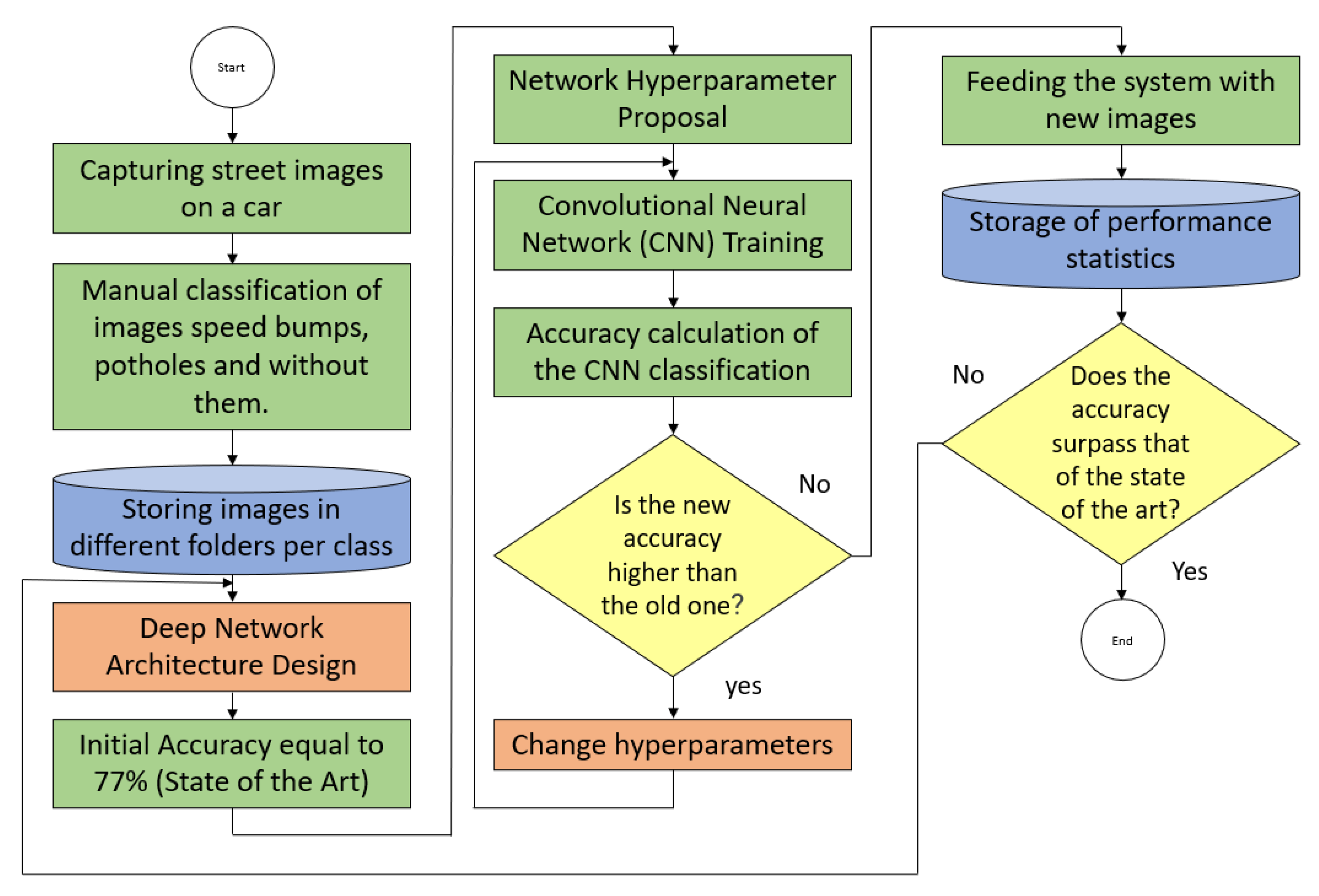
Maeda et al. presented a study to address road damage detection issues [9]. A large-scale road damage dataset was prepared, and images were captured using a smartphone installed on a car. Next, they used convolutional neural networks to train the damage detection system with their database and compared the accuracy and runtime speed on a GPU server and a smartphone. The accuracy reached was 75%. Shah and Deshmukh [7] attempted to identify the road surface by classifying it into potholes, speed bumps, and normal road from image data. The clasification of the road surface from the images, utilizing convolution neural network ResNet-50, is discussed. The images are hand-classified into the three classes, and these are used to train the neural network, achieving a true positive rate of 88.9%. Kennedy-Babu et al. [21] proposed two speed bump-detection methods: (i) Otsu’s threshold and (ii) morphological operation. These processes are superior to the existing ones because they do not utilize any external information network, so they are free from GPS error, network overload, delay, and incorrect alarm. The proposed Otsu’s approach is straightforward, efficient, and yields 74.6% accuracy. The performance of the morphological or structural operation achieves good results, with an 85.8% detection ratio. The two proposed designs provide a higher than 90% detection rate for properly painted roads and optical illusion-type speed bumps. Another contribution is the investigation of Asad et al. [22], which classified a dataset of images with potholes in various road conditions and lighting variations. They tested various deep learning architectures such as Tiny-YOLOv, YOLOv4, and YOLOv5, with accuracies of 80.04%, 85.48%, and 95%, respectively. The study found Tiny-YOLOv4 to be the best model for pothole detection, with 90% detection accuracy.

1.4. Our Proposal

A relevant problem detected in studies such as [14,17,18,20,21] was that their systems focused on detecting well-marked speed bumps; for this reason, they presented difficulties during the detection of unmarked speed bumps. Our system is capable of detecting marked and unmarked speed bumps with a balanced success rate. This is an important aspect in the Mexican environment because many speed bumps are not marked. Also, the way that our system processes the images differs from most current convolutional networks because it does not perform a stride in the convolution layer in order not to under-sample and thus hide detailed information about the input image. Although the amount of processing at the input is greater than in other architectures, we tried to use the fewest number of network layers so as not to compromise the processing speed of the deep network. In contrast to various works in the literature, our proposal manages to detect both speed bumps and potholes [2] for car traffic, and the work methodology that we follow is illustrated in the flowchart of Figure 1.
In this article, we propose the use of a deep neural network without strides or pooling but with a “batch normalization” layer to classify images that contain a pothole or speed bump, as well as those that do not. This is in conjunction with a manually labeled database obtained from ZED camera videos on avenues in the city of Celaya, Guanajuato, Mexico, in order to help autonomous driving systems and human drivers prevent road accidents due to speed bumps and humps.

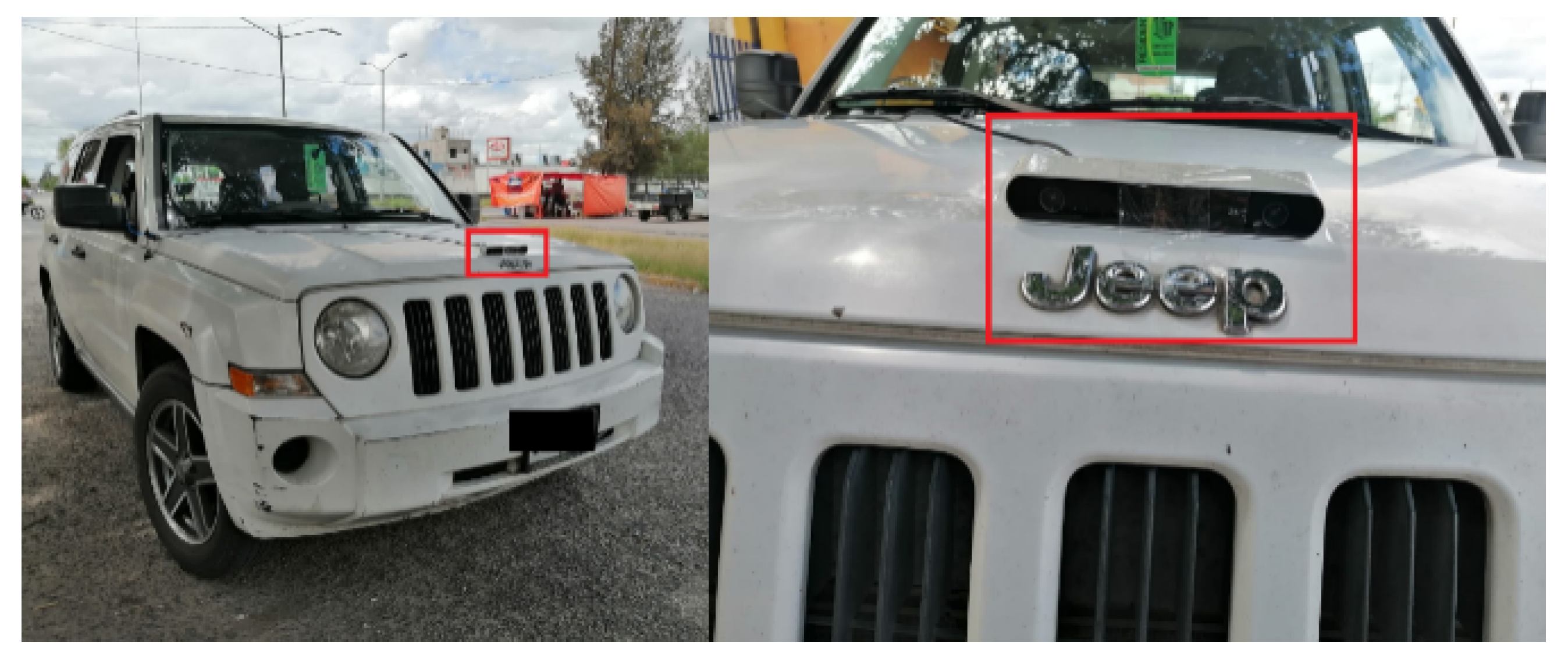
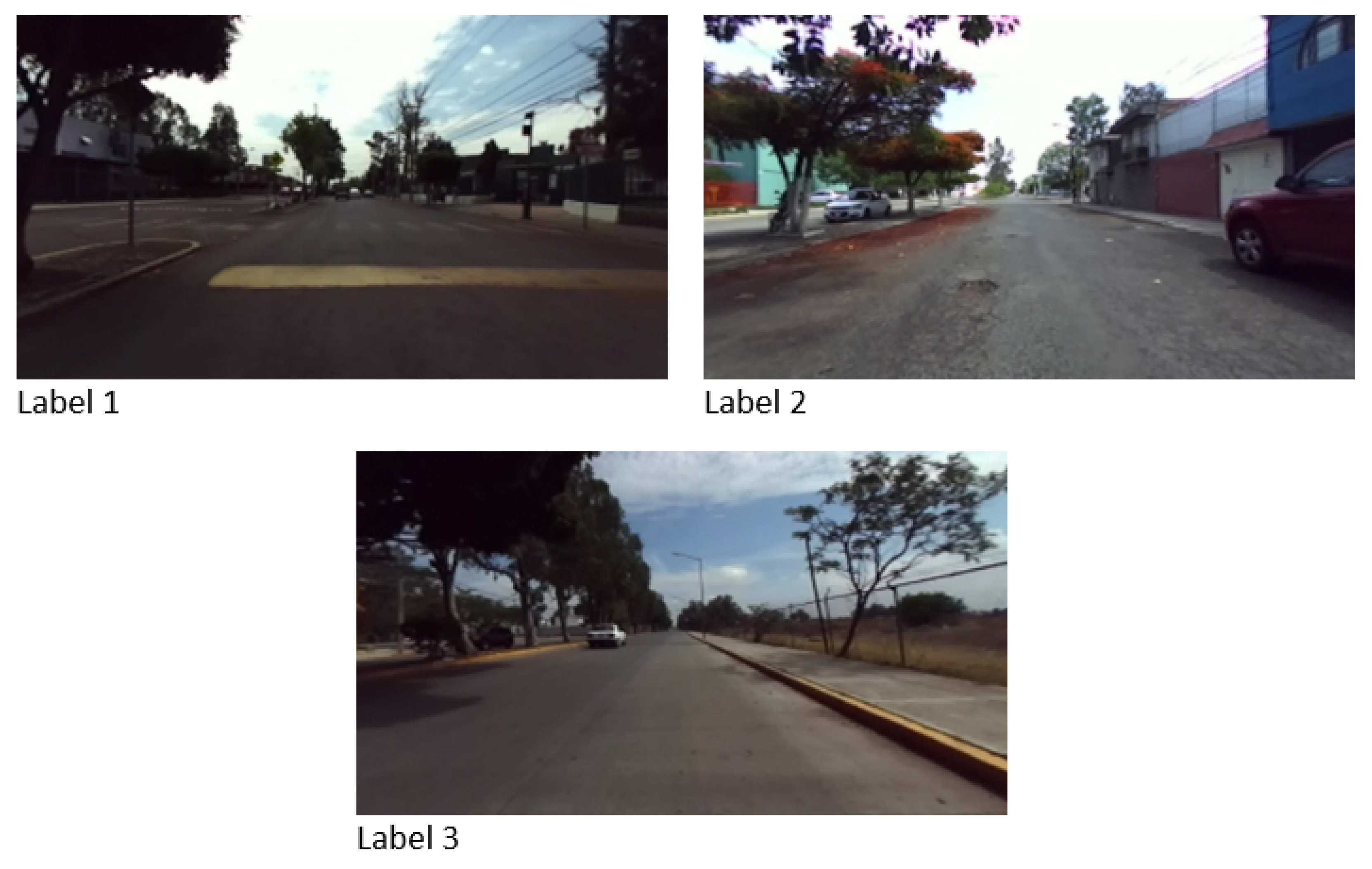
2. Materials and Methods

The software used in this work was MATLAB 2019a, along with its Deep Learning toolbox, running on a Windows 10 Pro operating system on hardware equipped with an Intel(R) Core(TM) i9-10900X CPU @ 3.70 GHz 3.70 GHz processor, manufactured in Dalian, Liaoning, China.
A database was constructed using a ZED camera [23] mounted on the front of an SUV, as shown in Figure 2. The tour to take the photographs was conducted in the city of Celaya, Guanajuato, Mexico. A total of 179 images of bumps were collected and stored in folder 0 (134 yellow speed bumps and 35 unmarked speed bumps); 231 images of potholes were stored in folder 1; and 304 images of streets without bumps or potholes were stored in folder 2. The images were captured at a resolution of 376 × 672 pixels. One of the most important factors when selecting the images was the position of the sun. For example, around six in the afternoon, the sun sometimes shone directly into the camera and hindered the capture of good-quality images. Therefore, it was necessary to eliminate such images, as well as some images that did not contain speed bumps or potholes, to balance the number of images in each class.
Three categories stored in different folders were used to label the images: an image with label 1 has a speed bump, an image with label 2 has a pothole, and an image with label 3 has no speed bump or pothole. Examples of this type of image are shown in Figure 3. It is important to note that, in the database, there are speed bumps that are not marked and others that are marked in yellow. Some have yellow stripes, and others are completely painted yellow. The potholes, which are not desired characteristics of the streets, are not marked and could be confused with puddles of water on the streets.

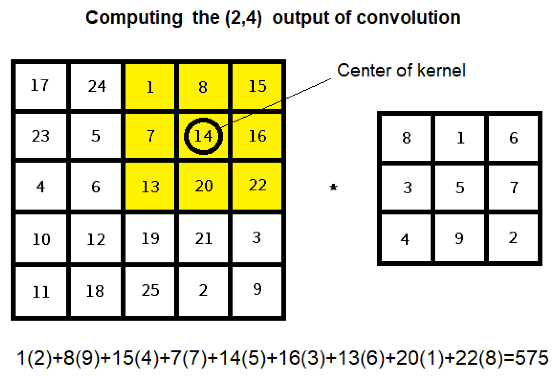
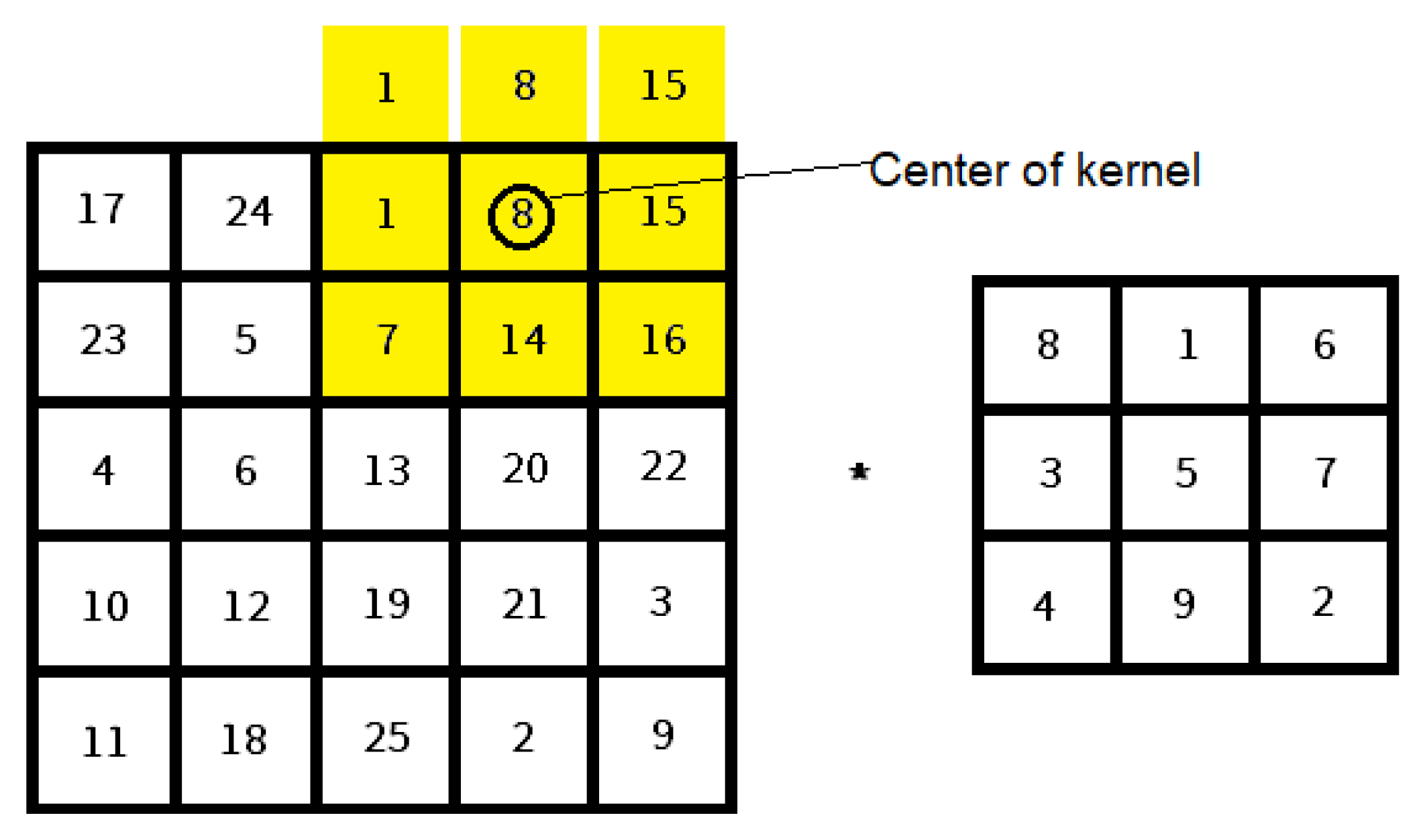
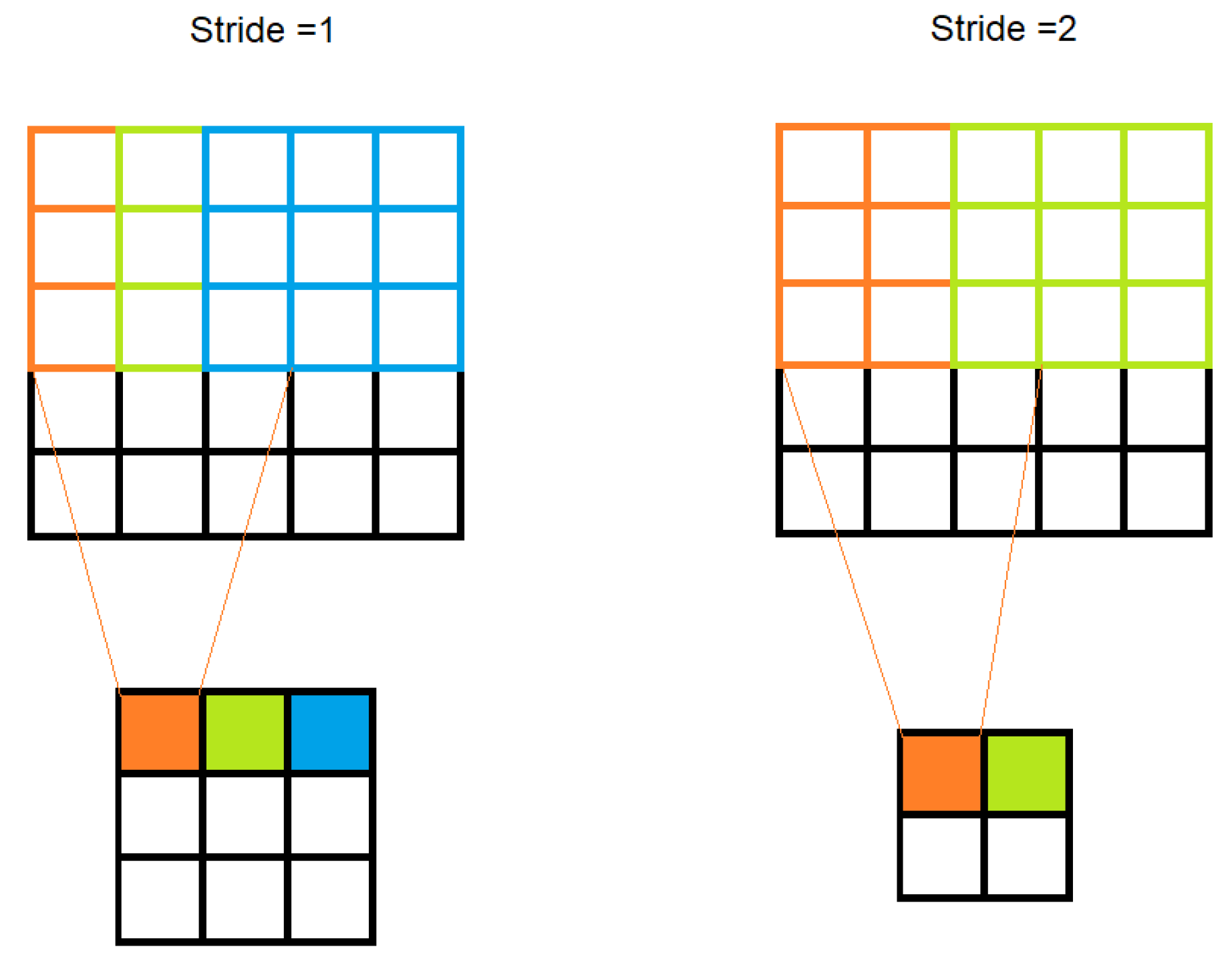
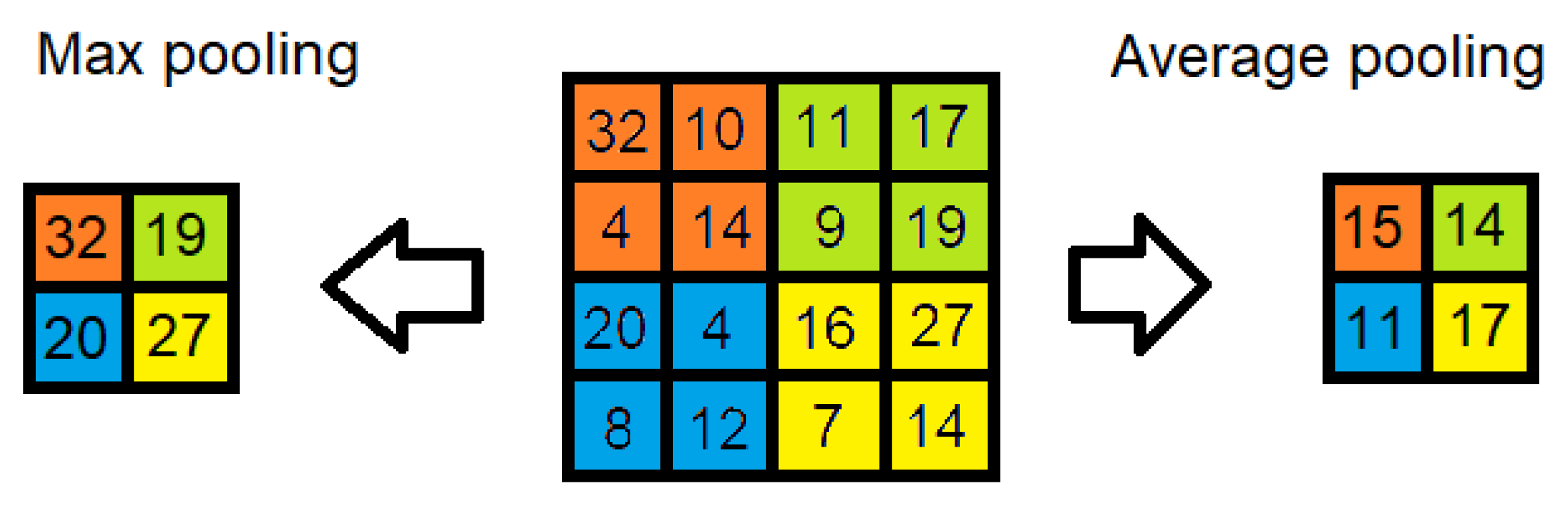
2.1. Basics of Deep Learning in Images

Deep learning is a set of machine learning algorithms that models high-level abstractions on large amounts of data using multiple iterative nonlinear transformations of data expressed in matrix or tensor form. A typical architecture in this scheme for image understanding is a convolutional neural network (CNN) that is organized in layers. Usually, the first layers perform convolution operations and the last one has a fully connected neural network.
Linear filtering of an image is accomplished through an operation called convolution indicated by ∗ and also expressed as (4), (5) and (6) for color images. This is an operator in the neighborhood of each pixel, where the output is the weighted sum of neighboring input pixels. The weight matrix is called the convolution kernel or filter. For example, Figure 4 illustrates how a pixel resulting from the convolution is calculated when filtering it with a 3 × 3 kernel in position (2, 4).
When an output pixel at the edge of an image is computed, a portion of the convolution falls outside the image edge, as illustrated in Figure 5. The padding of pixels outside the image to complete the processing of the image convolution is simply called “Padding”. If set to “same”, MATLAB calculates the padding value at training time so that the output is the same size as the input when stride is equal to 1.
On the other hand, stride operation controls the jumps of the filter on the input image in pixels. If the stride is set to 1, the filter moves 1 pixel at a time, and if the stride is 2, the filter moves 2 pixels at a time. The higher the stride value, the smaller the size of the resulting output image, as shown in Figure 6.
The pooling operation reduces resolution of the feature map by reducing its height and width, while retaining features of the map required for classification. This is called down-sampling. Figure 7 shows an example of this process.
For several decades in image processing, convolution has been used to filter images, segment them, improve their contrast, and even classify them. However, this processing is a very data-heavy task, which is why stride and pooling operations are used to subsample data; however, these processes waste the high quality of the current images.

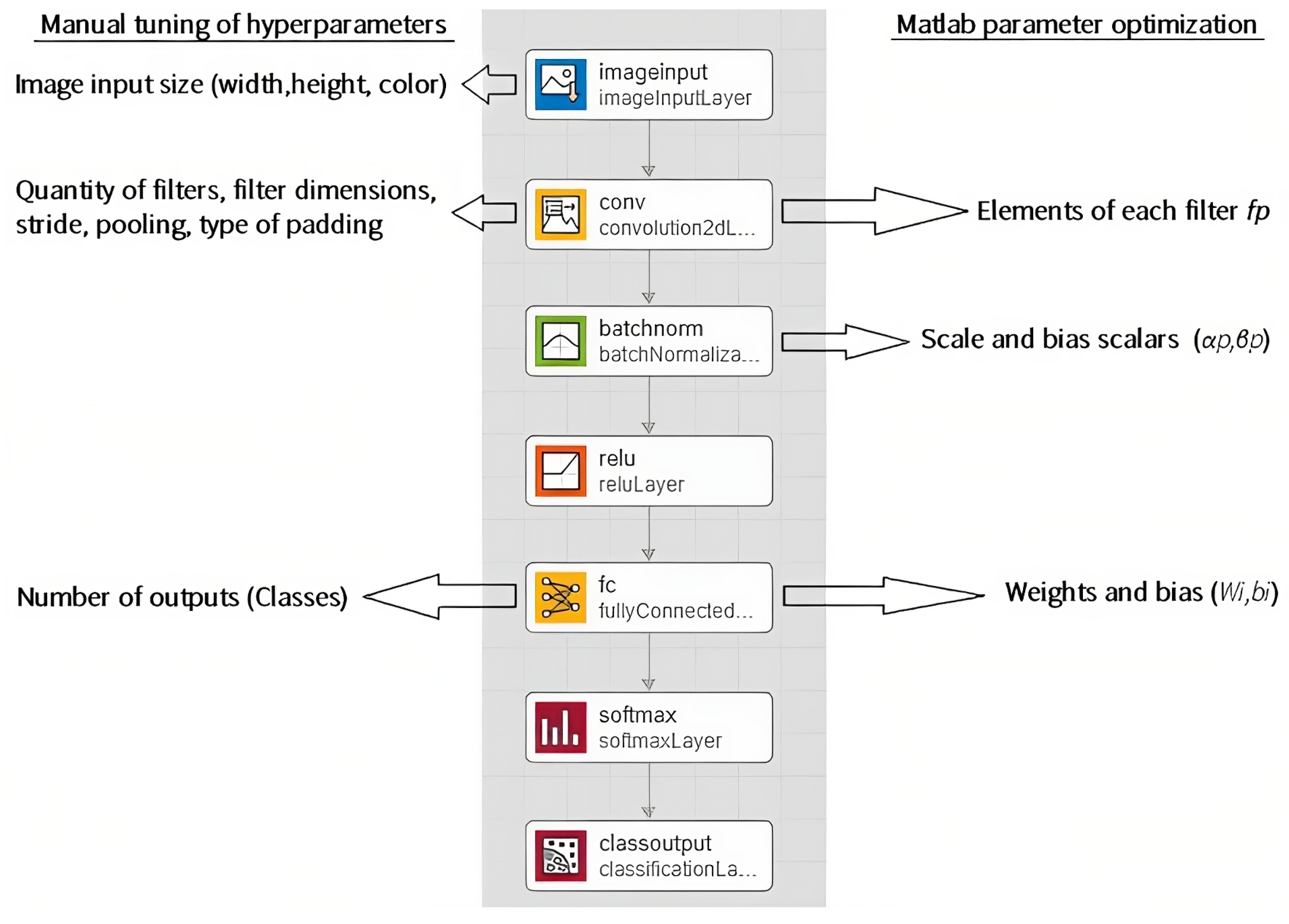
2.2. Convolutional Neural Network Architecture

First, a color image is received from the camera with resolution k × l × c ( k = 672 columns, l = 376 rows, and c = 3 for RGB color index), with 8 bits of resolution for each pixel and the RGB color scheme expressed as:
I ( x , y , z ) 0     Z   255 x | 1     x     k , y | 1     y     k , z | 1     z     k
where I is a three-dimensional matrix. The first layer, named “ImageInputLayer”, creates a data normalization function that subtracts the mean image ( m e a n I ) of the training set (for this case, the maximal n is 714) from each input image for color images with dimensions of 376 in height, 672 in width, and 3 for color in the RGB format, stored in a (376,672,3) tensor.
m e a n I = I 1 + I 2 + . . . + I n n
I ^ n = I m e a n I
The second layer, “Convolution2Dlayer”, is a convolutional layer with 37 convolution filters of width and height 3 × 3 ( f 1 , f 2 ,…, f p = 37 ), with s t r i d e = 1 and without pooling, but with a padding t y p e = " s a m e " to capture image details and avoid subsampling the scene information, stored in a (376,672,3,37) tensor.
C O N V p ( x , y , 1 ) = d x = a a d y = b b f p ( d x , d y , 1 ) I ^ n ( x d y , y d z , 1 )
C O N V p ( x , y , 2 ) = d x = a a d y = b b f p ( d x , d y , 2 ) I ^ n ( x d y , y d z , 2 )
C O N V p ( x , y , 3 ) = d x = a a d y = b b f p ( d x , d y , 3 ) I ^ n ( x d y , y d z , 3 )
where f p is a convolution window of size ( 2 a + 1 ) by ( 2 b + 1 ) . And d x and d y are the indices that traverse the window on the x and y axes.
The third layer, “batchNormalizationLayer”, normalizes a mini-batch of data across all observations for each feature independently to accelerate training of the convolutional neural network and reduce sensitivity to network initialization. It is recommended to use batch normalization layers between convolutional layers and non-linearities, as in our case, where we use a ReLU layer after a convolutional layer, stored in a (376,672,3,37) tensor.
C ^ p ( x , y , z ) = C O N V p ( x , y , z ) μ p σ p
C N ^ p ( x , y , z ) = α p C ^ p ( x , y , z ) + β p
where μ p is the mean, σ p the standard deviation, α p an amplification parameter, and β p a bias value for each feature.
The fourth layer, “ReluLayer”, is a rectified linear unit (ReLU) that performs a thresholding operation on the input. Values less than zero are set to zero, and values greater than zero remain their value. Compared to the tanh (hyperbolic tangent) and sigmoidal functions, ReLU has no saturation zones. These saturation zones mean that the output of the neurons does not change significantly, which causes the training gradient to not change and network parameters to not undergo significant changes. This generates a stagnation in the training process. That is the reason why the ReLU function has gained relevance in current neural networks, stored in a (376,672,3,37) tensor.
R e L U ( x , y , z ) = m a x ( 0 , C N ^ p ( x , y , z ) )
The fifth layer, “fullyConnectedLayer”, creates a fully connected neural network with an output size of 3 because it is being classified into that number of classes ( i = 1 , 2 , 3 ). The output of the ReLU layer is vectorized ( v e c ( ) ); that is, the matrix is converted to a vector with all the elements of the matrix, an operation also known as flattening. This layer multiplies its inputs by an array of weights W i and then adds a bias vector b i ; the result is applied to the input of a tansig function. It means that our full connected neural network has 28,046,592 inputs and 3 outputs (28046592,3).
F C L i = v e c ( R e L U ( x , y , z ) ) W i + b i
The sixth layer (3 inputs, 3 outputs), “SoftMax”, also uses a softmax function, which is typically used as the final layer of classifiers based on neural networks. It converts a vector of N real values into a vector of N real values that sum to 1, allowing for interpretation as probabilities. In our case, N = 3 .
s o f t m a x ( F C L ) i = e F C L i j = 1 N e F C L j .
The seventh and last layer, “classOutput” (3 inputs, 3 outputs) is the classification layer. It computes the cross-entropy loss of the classification outputs as mutually exclusive classes (3,3).
l o s s = 1 M n = 1 M i = 1 K g i t n i l n ( q n i )
where M is the number of samples, K is the number of classes, g i is the weight for class i, t n i is the indicator that the nth sample belongs to the ith class, and q n i is the output for sample n for class i, which in this case is the value from the softmax function. In other words, q n i is the probability that the network associates the nth input with class i. The complete deep learning network architecture can be seen in Figure 8 with respective parameters and hyperparameters.

2.3. Hyperparameter Tuning

Hyperparameters in CNN are the high-level parameters of the architecture; for example, the size of the input image, the number of convolution filters to use, the size of the convolution filters, the number of neural network outputs, among others. These are defined before training it. On the other hand, the network parameters are the values that are chosen automatically by an optimization algorithm implemented by MATLAB; in our case, this is the SGDM (Stochastic Gradient Descent with Momentum Optimizer) as the weights of the neural network and the values of the elements of the convolution filters.
Computer hardware is very relevant for training deep neural networks, especially when using GPUs for performing the iterations [24]. However, it is necessary to optimize the network architecture by tuning its hyperparameters and starting with an appropriate database. Simply increasing the depth of the network does not always result in better performance or better feature learning. Therefore, if the categories are highly discriminable, very deep architectures may not be required. On the other hand, using a larger input volume during training can improve filter learning for different categories, even though the computational cost can be significant. Considering that the network’s main task is prediction, using high-performance equipment becomes an intermediate step. The final application can run on low-cost embedded systems, such as a Raspberry Pi. To find the right architecture, it is crucial to make gradual changes to a single parameter at a time, allowing for the correct analysis of its effect on training.

3. Results

In this section, the accuracies of various deep neural network architectures are presented to determine the best one. Only the hyperparameters of the convolution layer were varied, since it is the most computationally intensive layer. After conducting several experiments with different filters, the best architecture was identified, and only some of the results are presented. Figure 9 depicts the training and validation progress, as well as the accuracy of the proposed deep neural network (Model 1) for detecting speed bumps and potholes in our database. In this case, 36 filters of dimensions 5 × 5 were used.
Figure 10 shows the progress of training and validation, as well as the accuracy of the proposed deep neural network called Model 2. It used 37 filters of 5 × 5 pixels, with an accuracy of 92.06%.
Figure 11 shows the progress of training and validation, as well as the accuracy of the proposed deep neural network called Model 3. It used 38 filters of 5 × 5 pixels, with an accuracy of 64.95%.
Figure 12 shows the progress of training and validation, as well as the accuracy of the proposed deep neural network called Model 4, which used 37 filters of 7 × 7 pixels, with an accuracy of 57.94%.
Figure 13 shows the progress of training and validation, as well as the accuracy of the proposed deep neural network called Model 5, which used 37 filters of 3 × 3 pixels, with an accuracy of 98.13%.
Figure 14 shows the progress of training and validation, as well as the accuracy of the proposed deep neural network called Model 6, which used 38 filters of 3 × 3 pixels with an accuracy of 83.18%.

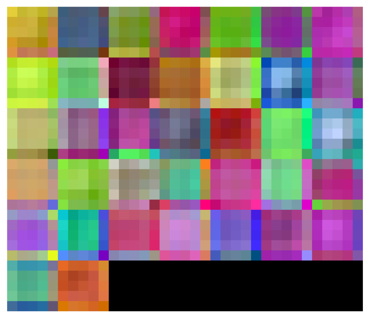
Feature Visualization of Convolutional Neural Network

Convolutional neural networks use filters that extract complicated features from a window of 3 × 3, 5 × 5, to p × p , where p is usually odd. The network learns these characteristics automatically during the training or optimization process. What the network learns during training is sometimes unclear. However, MATLAB provides functions to be able to visualize the learned functions. The outputs of the fully connected layers at the end of the network correspond to high-level combinations of the features learned by the previous convolution layers. In the case of our CNN proposal, it shows the features obtained in layers 2, 3, and 4 in Figure 15, Figure 16 and Figure 17.

4. Discussion

The results show that there are different architectures and that the best one is Model 5, with a precision of 98.13%. It can also be observed that, when the number of filters is varied in 5 × 5 windows, the best result is obtained with 37 filters. When the number of filters is fixed at 37 and the filter size is varied, the best result is obtained with a size of 3 × 3. However, increasing the number of filters to 38 with a 3 × 3 filter size leads to a decrease in precision to 83.18%, as shown in Table 2. Therefore, we selected Model 5.
Pothole and bump detection systems based on images provide us with the opportunity to predict the presence of these anomalies on the road in order to avoid them. In contrast, accelerometers do not allow this because they require a very sudden movement to detect a pothole or speed bump.
On the other hand, when we compared our proposal with similar works, we identified several articles that detected potholes and speed bumps using accelerometers, lidar, and images. However, the closest works to ours were those proposed by Maeda et al., and by Asad et al. [9,22]. The first proposed a system on a smartphone running Inception V2 to detect potholes in Czech, Indian, and Japanese cities. Although they reported that their dataset was composed of 9053 road damage images captured with a smartphone, unfortunately, that dataset only contained images of potholes photographed from inside the car, not from the angle of a camera on a car to detect or predict the existence of anomalies on the road. The second proposed an image classification with potholes that were specifically photographed, which does not allow for capturing the conditions in which a driver would observe a pothole in the distance from a car. However, it is also a lightweight architecture that has eight layers of image processing.
In contrast, our database includes three types of images: those with speed bumps, with potholes, and without either. Moreover, the images were taken from the front of a car. Our deep neural network uses only 7 layers, which is lighter for the processing hardware compared to Inception V2 with 12 layers. Our proposal achieves an accuracy of 98.13%, whereas that of Maeda et al. reaches only 77%, as shown in Table 3. Unlike other works in the same vein, we do not use strides or pooling to extract all possible information. We also use a “BatchNormalization” layer to accelerate the training and decrease the sensitivity to network initialization, which other architectures do not use. In addition, we use a “SoftMax” layer, which allows for the output of the fully connected network to be interpreted as probabilities. The use of small 3 × 3 windows gives us the advantage of obtaining more image details.
Table 3. Comparison of different proposals of the state of the art.
ReferenceDataset SizeAccuracyDetected Anomalies
Maeda et al. [9]9053 images77%Potholes
Asad et al. [22]665 images95%Potholes
Our proposal714 images98.13%Potholes and Speed bumps

5. Conclusions

A deep neural network for the detection of speed bumps and potholes was successfully designed using images captured by a ZED stereoscopic camera placed on the front of an SUV. This system has the potential to improve the safety of automated and human drivers. The high degree of precision achieved during the validation process is satisfactory, and the database is unique for capturing the specific situation of the streets of Celaya, Guanajuato, Mexico. The deep convolutional network architecture only consists of seven layers, which makes it light to implement in embedded and high-performance computing systems. The proposed methodology takes advantage of all the information coming from the camera at its maximum resolution because no stride or pooling process is performed. Compared to other larger architectures, better results were achieved with fewer flops. Unlike other architectures, ours can classify potholes and speed bumps. As future work, we aim to increase the size of the database to include special cases and to implement this method in an integrated system, making it easily accessible for use on board cars. Another convenient future work is to implement the architecture parallelization using GPU and/or FPGA hardware. We believe that this system has great potential for further development and can make a significant contribution to improving road safety.

Author Contributions

Conceptualization, A.-I.B.-G. and J.-E.P.-L.; methodology, J.-A.P.-M.; software, J.-A.M.-V.; validation, D.L.-M. and M.-J.V.-A.; formal analysis, F.-J.P.-P.; resources, J.P.-O.; data curation, D.L.-M.; writing—original draft preparation, J.-E.P.-L.; writing—review and editing, J.-A.M.-V. and J.-J.M.-N.; visualization, F.-J.P.-P.; supervision, J.-A.P.-M.; project administration, A.-I.B.-G.; funding acquisition, A.-I.B.-G. All authors have read and agreed to the published version of the manuscript.

Funding

This research was funded by CONACYT in Becas Nacionales and Sistema Nacional de Investigadores grants. A part of the APC was funded by TecNM en Celaya.

Data Availability Statement

The MATLAB code and the database can be found at the following link: https://drive.google.com/drive/folders/1ugaPdFtf5o2Wgreb2DTOBgVhdDk2uZAL?usp=share_link (accessed on 4 July 2023).

Acknowledgments

The authors would like to thank the TecNM collaborators for the support provided to build this research.

Conflicts of Interest

The authors declare no conflict of interest.

References

  1. Secretarĺa de Comunicaciones y Transportes de México. Estadĺstica de Accidentes de Tránsito; Secretarĺa de Comunicaciones y Transportes de México: Mexico City, Mexico, 2020; Available online: https://imt.mx/archivos/Publicaciones/DocumentoTecnico/dt79.pdf (accessed on 4 July 2023).
  2. Corro, I. Joven cae en zanja de Tláhuac con todo y coche; asegura que no habĺa señalización, VIDEO. El Universal, 8 March 2023. [Google Scholar]
  3. Al-Shargabi, B.; Hassan, M.; Al-Rousan, T. A Novel Approach for the Detection of Road Speed Bumps using Accelerometer Sensor. TEM J. 2020, 9, 469–476. [Google Scholar] [CrossRef]
  4. Bello-Salau, H.; Aibinu, A.M.; Onumanyi, A.J.; Onwuka, E.N.; Dukiya, J.J.; Ohize, H. New road anomaly detection and characterization algorithm for autonomous vehicles. Appl. Comput. Inform. 2018, 16, 223–239. [Google Scholar] [CrossRef]
  5. Celaya-Padilla, J.M.; Galván-Tejada, C.E.; López-Monteagudo, F.E.; Alonso-González, O.; Moreno-Báez, A.; Martĺnez-Torteya, A.; Galván-Tejada, J.I.; Arceo-Olague, J.G.; Luna-Garcĺa, H.; Gamboa-Rosales, H. Speed Bump Detection Using Accelerometric Features: A Genetic Algorithm Approach. Sensors 2018, 18, 443. [Google Scholar] [CrossRef] [PubMed] [Green Version]
  6. Martinez, F.; Carlos Gonzalez, L.; Ricardo Carlos, M. Identifying Roadway Surface Disruptions Based on Accelerometer Patterns. IEEE Lat. Am. Trans. 2014, 12, 455–461. [Google Scholar] [CrossRef]
  7. Shah, S.; Deshmukh, C. Pothole and Bump detection using Convolution Neural Networks. In Proceedings of the 2019 IEEE Transportation Electrification Conference (ITEC-India), Bengaluru, India, 17–19 December 2019; pp. 1–4. [Google Scholar]
  8. Varma, V.S.K.P.; Adarsh, S.; Ramachandran, K.I.; Nair, B.B. Real Time Detection of Speed Hump/Bump and Distance Estimation with Deep Learning using GPU and ZED Stereo Camera. In Proceedings of the 8th International Conference on Advances in Computing and Communication (ICACC-2018), Kochi, India, 13–15 September 2018; Volume 143, pp. 988–997. [Google Scholar]
  9. Maeda, H.; Sekimoto, Y.; Seto, T.; Kashiyama, T.; Omata, H. Road Damage Detection Using Deep Neural Networks with Images Captured Through a Smartphone. arXiv 2018, arXiv:1801.09454. [Google Scholar]
  10. Villaseñor-Aguilar, M.J.; Peralta-López, J.E.; Lázaro-Mata, D.; Garcĺa-Alcalá, C.E.; Padilla-Medina, J.A.; Perez-Pinal, F.J.; Vázquez-López, J.A.; Barranco-Gutiérrez, A.I. Fuzzy Fusion of Stereo Vision, Odometer, and GPS for Tracking Land Vehicles. Mathematics 2022, 10, 2052. [Google Scholar] [CrossRef]
  11. Tai, Y.-C.; Chan, C.-W.; Yung-Jen, H.J. Automatic Road Anomaly Detection Using Smart Mobile Device. In Proceedings of the 5th Conference on Artificial Intelligence and Applications (TAAI 2010), Hsinchu, Taiwan, 18–20 November 2010. [Google Scholar]
  12. Mednis, A.; Strazdins, G.; Zviedris, R.; Kanonirs, G.; Selavo, L. Real time pothole detection using Android smartphones with accelerometers. In Proceedings of the 2011 International Conference on Distributed Computing in Sensor Systems and Workshops (DCOSS), Barcelona, Spain, 27–29 June 2011; pp. 1–6. [Google Scholar]
  13. Salari, E.; Yu, X. Pavement distress detection and classification using a Genetic Algorithm. In Proceedings of the 2011 IEEE Applied Imagery Pattern Recognition Workshop (AIPR), Washington, DC, USA, 11–13 October 2011; pp. 1–5. [Google Scholar]
  14. Choi, J.; Lee, J.; Kim, D.; Soprani, G.; Cerri, P.; Broggi, A.; Yi, K. Environment-Detection-and-Mapping Algorithm for Autonomous Driving in Rural or Off-Road Environment. IEEE Trans. Intell. Transp. Syst. 2012, 13, 974–982. [Google Scholar] [CrossRef] [Green Version]
  15. Astarita, V.; Caruso, M.V.; Danieli, G.; Festa, D.C.; Giofrè, V.P.; Iuele, T.; Vaiana, R. A mobile application for road surface quality control: UNIquALroad. Procedia-Soc. Behav. Sci. 2012, 54, 1135–1144. [Google Scholar] [CrossRef] [Green Version]
  16. Kulkarni, A.; Mhalgi, N.; Gurnani, S. Pothole Detection System using Machine Learning on Android. Int. J. Emerg. Technol. Adv. Eng. 2014, 4, 360–364. [Google Scholar]
  17. Devapriya, W.; Babu, C.N.K.; Srihari, T. Advance Driver Assistance System (ADAS)-Speed bump detection. In Proceedings of the 2015 IEEE International Conference on Computational Intelligence and Computing Research (ICCIC), Madurai, India, 10–12 December 2015; pp. 1–6. [Google Scholar]
  18. Devapriya, W.; Babu, C.N.K.; Srihari, T. Real time speed bump detection using Gaussian filtering and connected component approach. Circuits Syst. 2016, 7, 2168–2175. [Google Scholar] [CrossRef] [Green Version]
  19. Srimongkon, S.; Chiracharit, W. Detection of speed bumps using Gaussian mixture model. In Proceedings of the 2017 14th International Conference on Electrical Engineering/Electronics, Computer, Telecommunications and Information Technology (ECTI-CON), Phuket, Thailand, 27–30 June 2017; pp. 628–631. [Google Scholar]
  20. Bharathi, M.; Amsaveni, A.; Manikandan, B. Speed Breaker Detection Using GLCM Features. Int. J. Innov. Technol. Explor. Eng. 2018, 8, 384–389. [Google Scholar]
  21. Babu, K.C.N.; Devapriya, W.; Srihari, T.; Nandakumar, R. Speed-bump Detection using Otsu’s Algorithm and Morphological Operation. Int. J. Emerg. Technol. 2020, 11, 989–994. [Google Scholar]
  22. Asad, M.H.; Khaliq, S.; Yousaf, M.H.; Ullah, M.O.; Ahmad, A. Pothole Detection Using Deep Learning: A Real-Time and AI-on-the-Edge Perspective. Adv. Civ. Eng. 2022, 2022, 9221211. [Google Scholar] [CrossRef]
  23. STEREOLABS. Available online: https://www.stereolabs.com/zed-2/ (accessed on 13 April 2023).
  24. Ssheshadri, Jetson Nano Developer Kit User Guide. 2788 San Tomas Expressway Santa Clara, CA 95051. 15 January 2020. Available online: https://developer.download.nvidia.com/assets/embedded/secure/jetson/Nano/docs/NV_Jetson_Nano_Developer_Kit_User_Guide.pdf?svGUDWZio7oyFzB5oJu3kMwIBZBEpJ84wuGMfPRRDnmA5gIgeFKtQ987wVYovaAMCJa4UR8deq0CLbvazMUVFAFxBjxIYCZq_Ws9iTdBPmL4HV89ellsIv1IceR5knK2ldDCWXys-t1rENTDFitQTKsDCg8G1cjlQR2_V3D2DgjvFs1u986stSY_XLruS-GJonI=&t=eyJscyI6ImdzZW8iLCJsc2QiOiJodHRwczovL3d3dy5nb29nbGUuY29tLyJ9 (accessed on 4 July 2023).
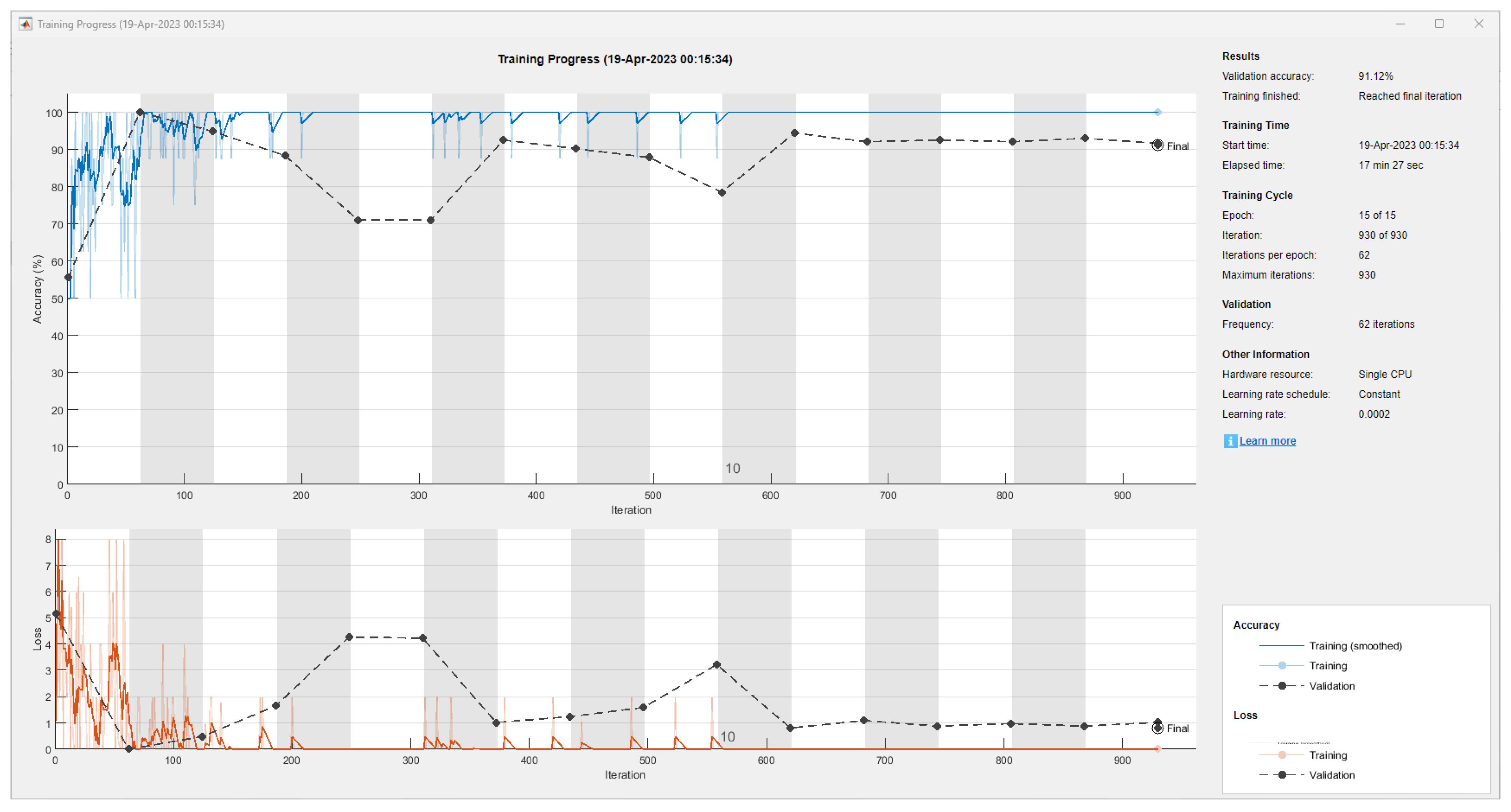
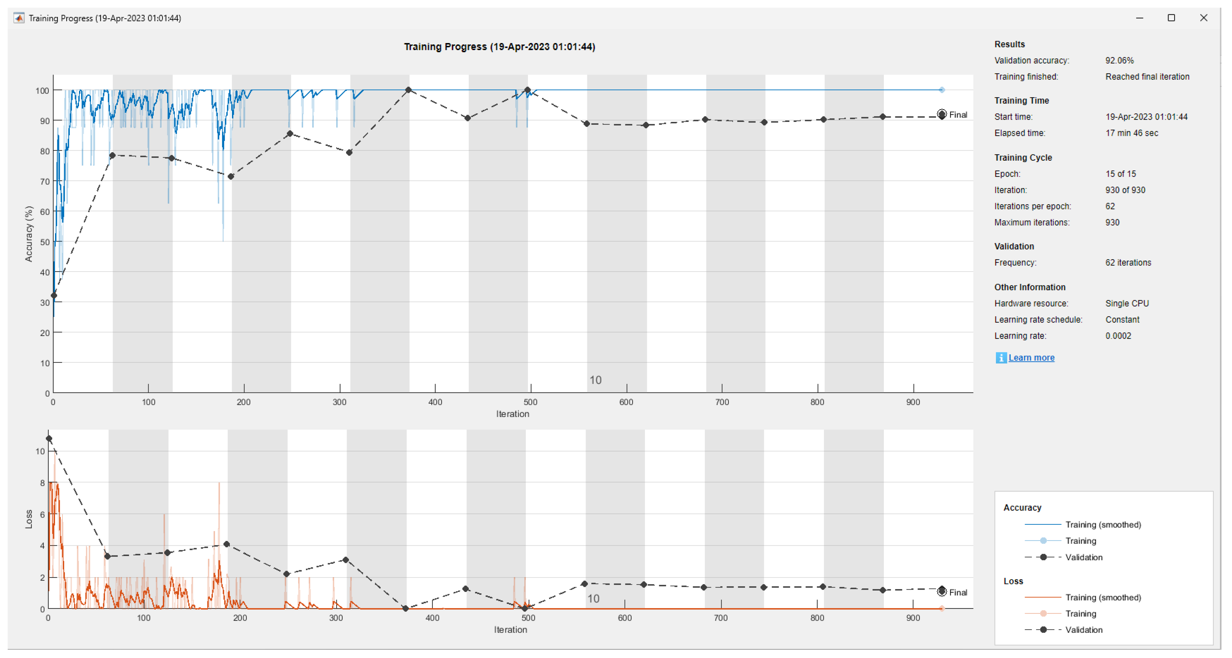
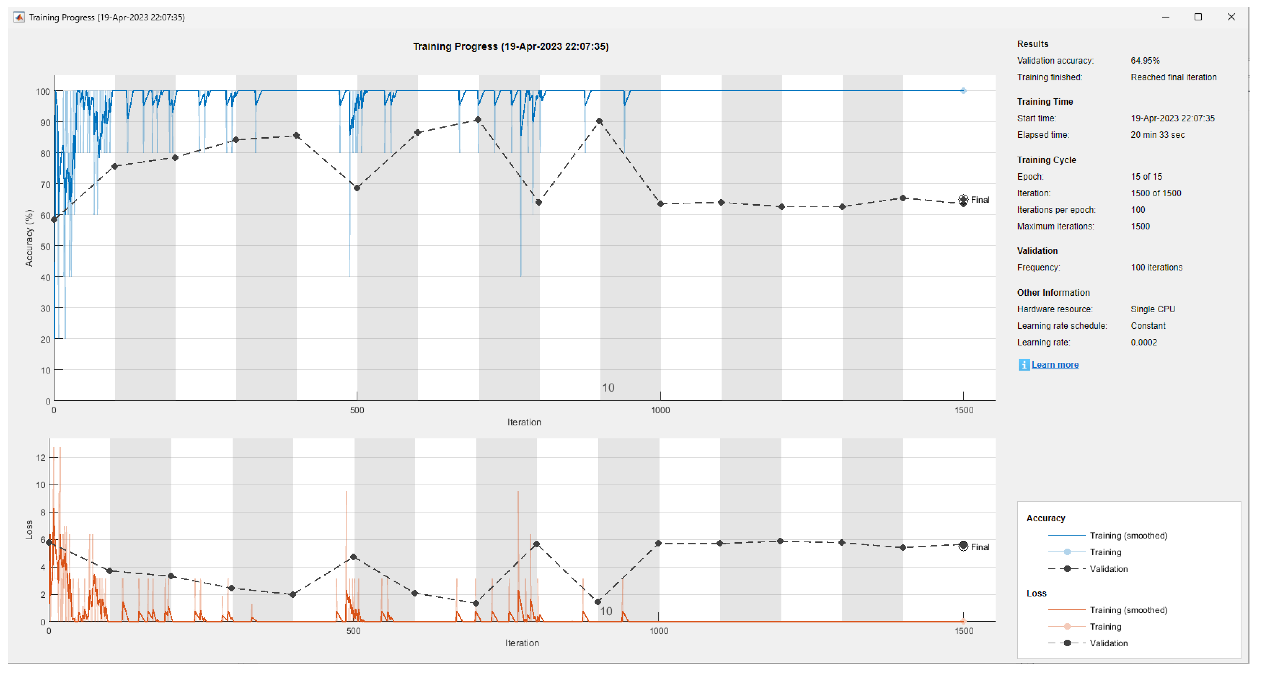
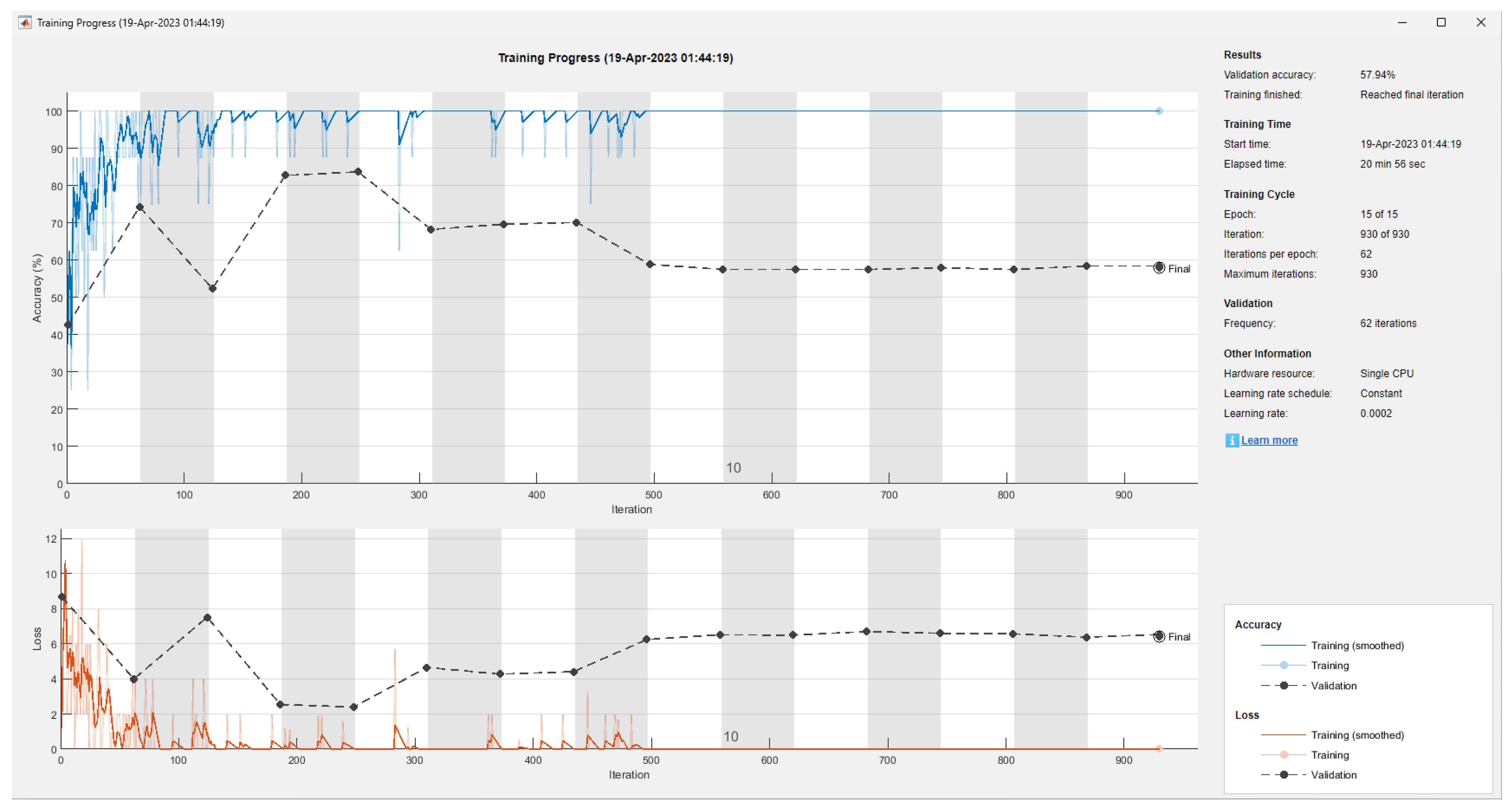
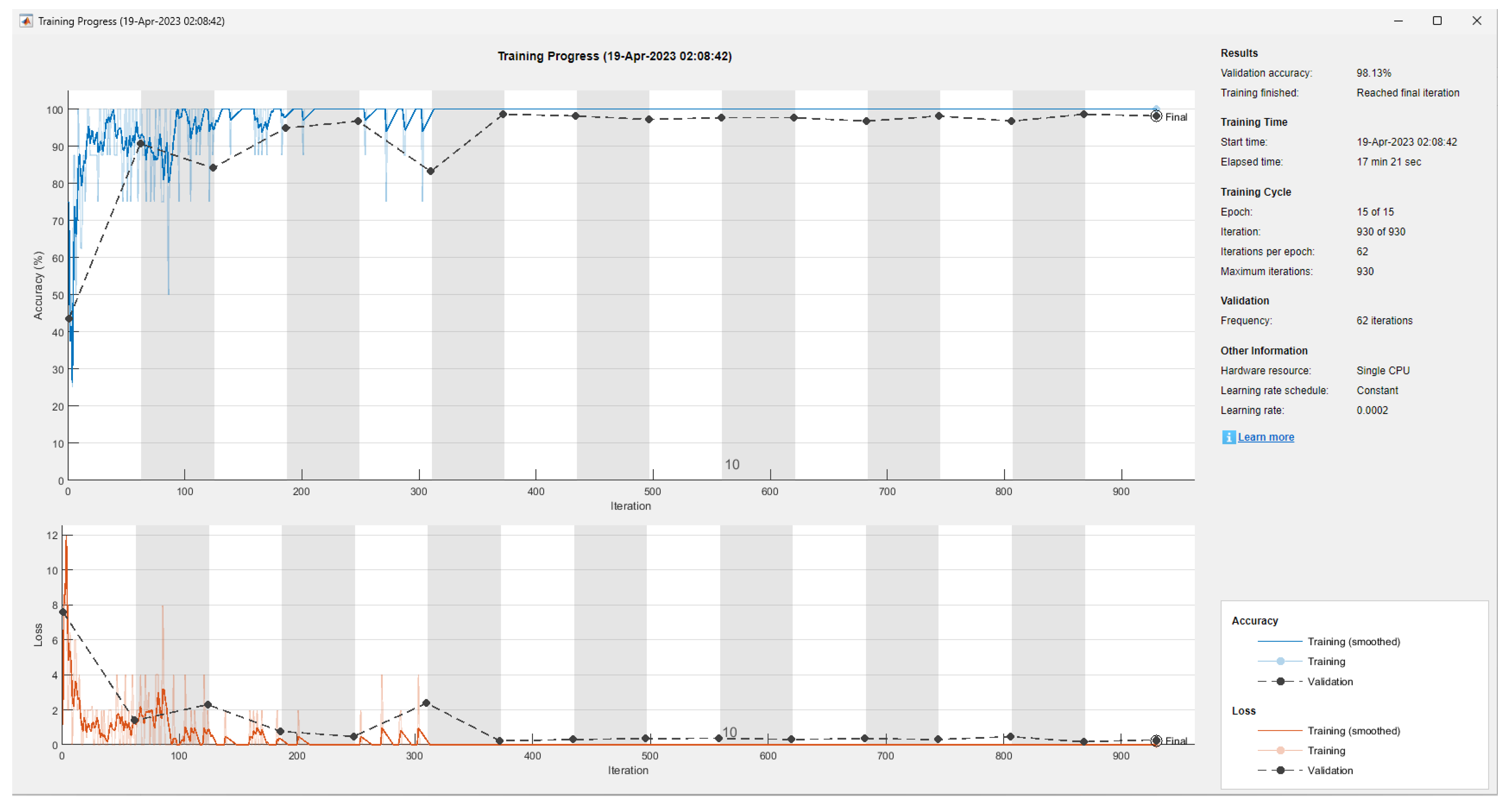
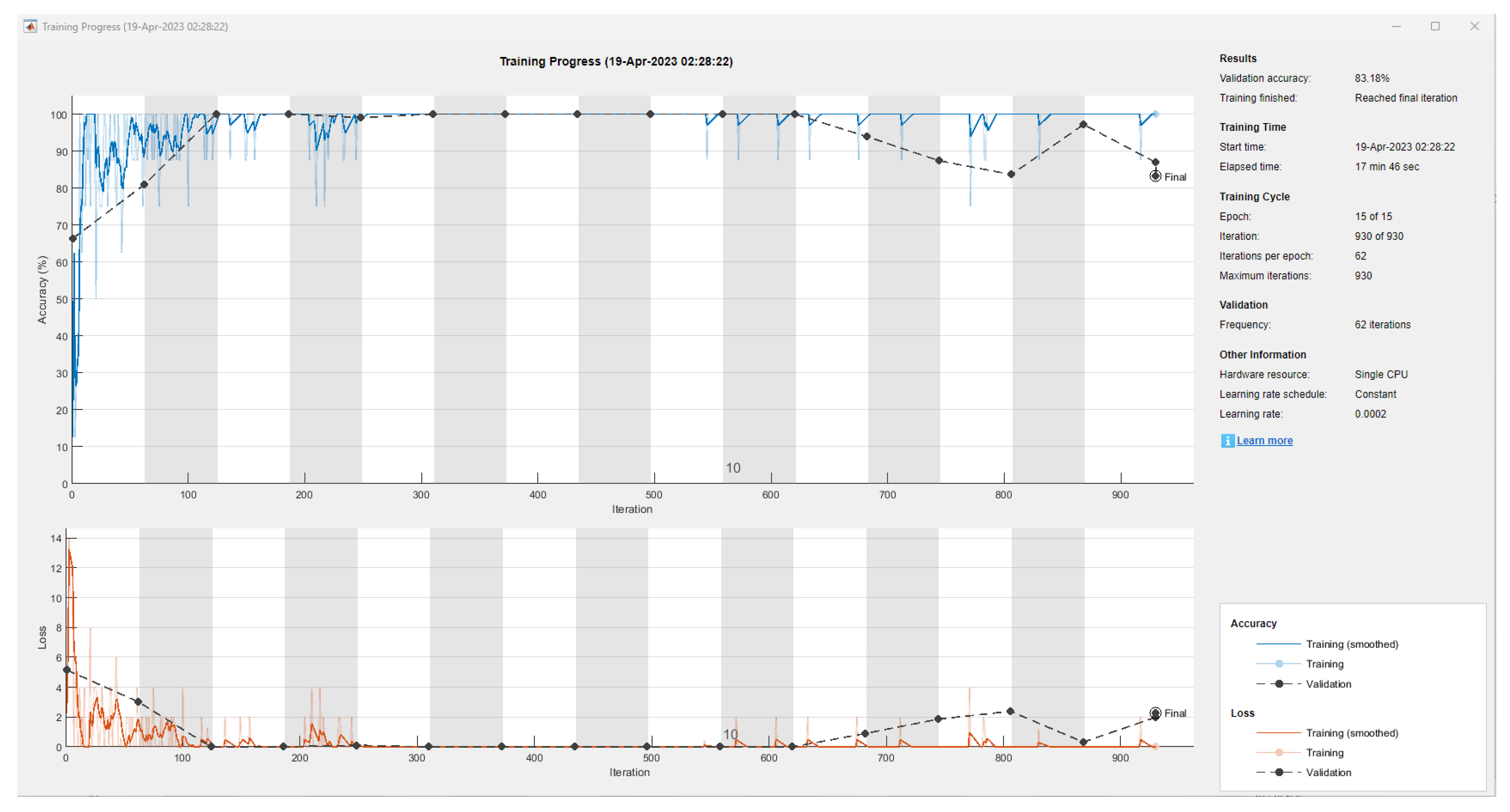
Figure 1. Proposal flowchart.
Applsci 13 08349 g001
Figure 2. ZED camera sitting on the car’s front.
Applsci 13 08349 g002
Figure 3. The three types of images to classify.
Applsci 13 08349 g003
Figure 4. The yellow area of the image is convolved (*) with the kernel (matrix) on the right and its result is 575.
Applsci 13 08349 g004
Figure 5. In “same” padding the border pixels are copied out in order to complete the convolution operation. In order to allow the center of the kernel to be applied to the edges of the image.
Applsci 13 08349 g005
Figure 6. The colors indicate the different types of strides that are made during the convolution. In stride = 1 we have two jumps while for stride = 2 we only have one jump.
Applsci 13 08349 g006
Figure 7. In each four pixels neighborhood of a different color, there are two types of pooling, the one on the left is the one that chooses the maximum and the one on the right is the one that calculates the average.
Applsci 13 08349 g007
Figure 8. Convolutional neural network architecture with their hyperparameters and parameters.
Applsci 13 08349 g008
Figure 9. Model 1: Neural network accuracy using 36 filters of 5 × 5 pixels, accuracy 91.12%.
Applsci 13 08349 g009
Figure 10. Model 2: Neural network accuracy using 37 filters of 5 × 5 pixels, accuracy 92.06%.
Applsci 13 08349 g010
Figure 11. Model 3: Neural network accuracy using 38 filters of 5 × 5 pixels, accuracy 64.95%.
Applsci 13 08349 g011
Figure 12. Model 4: Neural network accuracy using 37 filters of 7 × 7 pixels, accuracy 57.94%.
Applsci 13 08349 g012
Figure 13. Model 5: Neural network accuracy using 37 filters of 3 × 3 pixels, accuracy 98.13%.
Applsci 13 08349 g013
Figure 14. Model 6: Neural network accuracy using 38 filters of 3 × 3 pixels, accuracy 83.18%.
Applsci 13 08349 g014
Figure 15. Layer 2: 37 convolutional kernels of size 3 × 3 × 3 learned by the “2Convolution2Dlayer” on the 224 × 224 × 3 input images.
Applsci 13 08349 g015
Figure 16. Layer 3: 37 convolutional kernels of size 3 × 3 × 3 learned by the “batchNormalizationLayer” on the data from layer 2.
Applsci 13 08349 g016
Figure 17. Layer 4: 37 convolutional kernels of size 3 × 3 × 3 learned by the “ReluLayer” on the data from layer 3.
Applsci 13 08349 g017
Table 2. Accuracies of different convolutional network architectures.
ModelFilter SizeFilter QuantityAccuracyTraining and Validation Time
15 × 53691.12%17 min 27 s
25 × 53792.06%17 min 46 s
35 × 53864.95%20 min 33 s
47 × 73757.94%20 min 56 s
53 × 33798.13%17 min 21 s
63 × 33883.18%17 min 46 s
Disclaimer/Publisher’s Note: The statements, opinions and data contained in all publications are solely those of the individual author(s) and contributor(s) and not of MDPI and/or the editor(s). MDPI and/or the editor(s) disclaim responsibility for any injury to people or property resulting from any ideas, methods, instructions or products referred to in the content.

