Manipulator Smooth Control Method Based on LSTM-XGboost and Its Optimization Model Construction

Abstract

With the rapid development of computer and artificial intelligence technology, robots have been widely used in assembly, sorting, and other work scenarios, gradually changing the human-oriented mechanical assembly line working mode. Traditional robot control methods often rely on application fields and mathematical models, and they cannot meet the emerging requirements of versatility and flexibility in many fields, such as intelligent manufacturing and customized production. Therefore, aiming at the relationship between the manipulator’s smooth control command parameters and the manipulator’s actual motion stability in the multi-step object sorting task, this paper proposes a method for predicting the stability of the manipulator based on Long Short-Term Memory Extreme Gradient Boosting. The acquisition signal of the manipulator vibration is segmented according to the action, and the boost model is used to learn the relationship between the control command parameters and the stability characteristic indexes. Next, the Extreme Gradient Boosting algorithm establishes a feature index-stationarity score prediction model. The minimum Mean Absolute Error predicted by the five indicators is 0.0024 so that the model can predict the manipulator’s motion stability level according to the manipulator’s command parameters.

1. Introduction

In the stage of high-quality development of China’s economy, the development of the equipment and high-tech manufacturing industries is particularly prominent. According to the latest data from the National Bureau of Statistics, the added value of national industries above the designated size in 2021 is 9.6% higher than that in 2020, of which the added value of the high-tech manufacturing industry and equipment manufacturing industry increased by 18.2% and 12.9%, respectively. As a new alternative to artificial production tools, robots play a vital role in promoting the upgrading and development of high-tech manufacturing and equipment manufacturing [1,2,3]. Therefore, after putting forward the strategic goal of Made in China 2025, China has successively issued a series of documents to encourage the development of industrial robot technology. For example, in March 2021, the fourth session of the 13th National People’s Congress adopted the ‘Fourteenth Five-Year Plan for National Economic and Social Development of the People’s Republic of China and the Outline of the Vision Goals for 2035’, which proposes to implement intelligent manufacturing in depth, promote the development of the manufacturing industry in the direction of intelligence, and promote the innovative development of the robot industry; subsequently, in December of the same year, the Ministry of Industry and Information Technology issued the ‘14th Five-Year robot industry development plan,’ which also proposed to focus on promoting the development and application of industrial robots and other products and vigorously develop innovative products of industrial robots. At the same time, robots are used in industrial production lines [4,5,6,7]. According to the “2021 Industrial Robots” report published by the International Federation of Robots, China witnessed the installation of nearly 200,000 new robots in 2020. Furthermore, the total number of robots utilized in China by 2020 is projected to reach an impressive 94.3 million units, encompassing the entire industry.

In assembly and sorting tasks, robots are programmed to grab components and arrange them in a specific order within a box or on a conveyor, according to predetermined sorting rules or component installation guidelines. However, traditional robot control methods, such as teaching or offline programming, involve setting the robot’s motion trajectory or action posture in advance [8,9,10,11]. This approach works well when dealing with consistent elements and rules. However, as new components or boxes are introduced, or even when sorting rules change, a critical question arises: can the robot adapt to this new working environment and complete similar multi-step sorting tasks? While these traditional methods have served us well, the rapidly changing nature of work environments presents new challenges. In these scenarios, traditional teaching or offline programming control methods struggle to analyze and model complex and unstructured work environments. This difficulty can lead to incomplete tasks and wasted time, human resources, and material resources. To address this, robots should move beyond repeating pre-programmed actions. Instead, they should learn how to plan and perform tasks according to the new working environment and production requirements. In essence, we need to enhance the intelligence of robots to quickly respond to user needs. By doing so, robots will be able to handle sorting tasks effectively, even in complex and ever-changing scenarios.

With the rapid development of technology and industrialization, the robot industry has become one of the most critical industries in the world. In recent years, the scale of China’s robot industry has also been expanding. According to statistics, the scale of China’s robot market will reach 83.9 billion in 2021, with a broad prospect. With the industrial robot industry’s development, product quality has also put forward higher requirements. In this context, the research on performance evaluation and quality inspection of industrial robots has become the focus of experts and enterprises in related fields. The serial manipulator is one of the most widely used industrial robots. It has a high degree of freedom and can complete the handling and assembly work through instructions. It is widely used in vehicle manufacturing, electronic assembly, and other fields. Many domestic scholars have also proposed various robot control strategies for different application scenarios [12,13,14,15]. The deep deterministic policy gradient algorithm (DDPG) is used to control the robot arm to complete the action of object picking in a three-dimensional simulation environment. Compared with the manual debugging of the robot arm to achieve object picking, it takes much time. The use of deep reinforcement learning technology shortens the debugging time, and the algorithm after training is adaptive. The deep deterministic strategy gradient algorithm is used to solve the manipulator end control accuracy problem. To enable the manipulator to open the valve without being limited by the size of the valve handwheel, the model of the rotating valve handwheel is established based on the Markov decision process, and the state space and reward function are designed based on the relative position relationship between the end effector of the manipulator and the edge of the valve. Without the support of the kinematics model and dynamics model theory, the robot learns a deterministic grasping strategy through deep reinforcement learning to complete the task of grasping the moving target in space.

With the application of the manipulator in various industrial fields, the requirements for its stability have gradually increased. The hardware manufacturing process, motion trajectory planning algorithm, and command parameter setting of the manipulator may lead to different degrees of jitter in the working process of the manipulator, which affects its working quality and efficiency [16,17,18,19,20]. Therefore, it is necessary to predict the stability of the manipulator. Currently, the research on the stability of industrial manipulators is mainly analyzed from the perspective of dynamic modeling, the trajectory planning algorithm, vibration suppression, and the less direct quantitative evaluation and prediction of its stability. The stability analysis of the manipulator is usually measured by the vibration generated by the movement of the manipulator. The standard vibration quantities include acceleration, velocity, and displacement [21,22,23,24,25]. In the research on mechanical arm vibration signal acquisition, it is proposed to segment the time series of the collected vibration signal according to the state. On this basis, anomaly detection is realized by analyzing the signal of each state. A wireless high-precision vibration sensor is developed to detect the state of the manipulator in real time. An industrial robot performance evaluation method based on the binocular vision of camera lenses is proposed, which improves the positioning accuracy of the end of the manipulator. The proposed synchronous measurement method of manipulator configuration and target pose improves the motion accuracy and working ability of intelligent cable-driven robots. In addition, the collected vibration signals of the manipulator need to be analyzed and extracted to study the stability [26,27].

Robotic manipulator control represents a significant challenge in the field of robotics due to the need for precise, safe, and efficient movement in a variety of tasks and environments. Among the many approaches used to model and predict the behavior of these manipulators, machine learning techniques have shown remarkable promise. Specifically, a hybrid model incorporating Long Short-Term Memory (LSTM) and eXtreme Gradient Boosting (XGBoost) has been the focus of recent research. LSTM, a type of Recurrent Neural Network (RNN), is known for its ability to learn and predict time-series data. It overcomes the shortcoming of traditional RNNs in handling long-term dependencies, making it a suitable choice for tasks that involve sequences with temporal dependencies, such as the motion of a robotic manipulator. On the other hand, XGBoost, an efficient implementation of gradient boosting machines, is appreciated for its capacity to capture complex non-linear relationships and its robustness against overfitting. The gradient-boosting algorithm focuses on minimizing the prediction error by adding new models to the ensemble sequentially.

In the realm of manipulator stability research, the prevalent approach is to enhance the path planning algorithm to suppress vibrations. Most methods tend to view stability as an optimization index rather than a target for evaluation. Separately, there are studies that use vibration directly as a stability evaluation index. However, these primarily focus on detecting manipulator anomalies, overlooking the stability prediction under regular operating conditions. This paper proposes a different approach. We extract the cumulative characteristics of action from the manipulator’s vibration signal subsequence. The command parameters of each action are processed to create a stability index evaluation system centered on a scorecard. Moving on, we construct a ‘command-feature index’ prediction model leveraging XG Boost. Subsequently, we introduce the variable-length LSTM algorithm to establish a ‘feature index-stationarity score’ prediction model. While the former predicts command-feature indices, the latter is used for forecasting stationarity scores. Lastly, we put our models to the test using the SR4B industrial manipulator data set. The results demonstrate that our models deliver accurate predictions, verifying their effectiveness.

2. Mechanical arm Stability Index System

The construction of an index system should be scientific and reasonable to make the evaluation results more reliable and effective. In the study of the stability of the manipulator, physical quantities such as vibration acceleration, time and torque are usually used to construct the index system. In this paper, the physical quantity of vibration acceleration is used as the basic quantity of the stability index, and the score card model is constructed on this basis. Based on the vibration acceleration, the absolute average vibration acceleration $|a{|}_{ave}$, the standard deviation of vibration acceleration δ_a, the peak acceleration $a_p$, the standard deviation of angular velocity δ_w and jerk can be obtained. Their calculation formulas are as follows [24].

$$|a{|}_{ave}=\frac{1}{N}\sum _{n=1}^N\left|a_n\right|$$

(1)

$${\delta }_{\mathrm{a}}=\sqrt{\frac{1}{N-1}\sum _{n=1}^N{\left[a_n-a_{ave}\right]}^2}$$

(2)

$$a_p=\max \left|a_n\right|$$

(3)

$${\delta }_w=\sqrt{\frac{1}{N-1}\sum _{n=1}^N{\left[w_n-w_{ave}\right]}^2}$$

(4)

$$\mathrm{jerk}=\frac{1}{T}\sum _{x,y,zt}\sum _{t=0}^T\left|\frac{\mathrm{d}a(t)}{\mathrm{d}t}\right|\mathsf{\Delta }t$$

(5)

where a represents the acceleration sequence of the main body of the manipulator, a_n and w_n represent the nth acceleration and angular velocity in the sequence, respectively, and the sequence length is N.

The scoring card model is a kind of risk grade evaluation model commonly used in the financial field. This paper uses the scoring card model to construct the manipulator stability scoring card. Because the construction process of the score card model is not the focus of this paper, only the final score table and its use method are given. The scoring table: After the vibration acceleration and angular velocity data of the manipulator are given, the values of δ_a, a_p, δ_w and jerk are first calculated by Formulas (1)–(5). The scores of each index are shown in

Table 1. Score Criteria.

Criteria	Value
$|a{|}_{ave}$	2.7139
δa	5.2828
ap	9.0056
δw	2.2541
jerk	55.7436

.

$$\mathrm{score}={\mathrm{score}}_{\mathrm{base}}+\sum _{i\in \mathrm{Index}}{\mathrm{scrore}}_i$$

(6)

where Index = {$|a{|}_{ave}$, δ_a, a_p, δ_w, jerk}, base score_base = 75.

3. Inverse Kinematics Problem Solving Method of Serial Manipulator

The problem of inverse kinematics in a serial manipulator is a fundamental aspect of trajectory planning. It necessitates the calculation of joint rotation angles and displacements based on the desired final position of the manipulator. Two prevalent strategies for solving this problem are the analytical and the numerical methods. The analytical method utilizes the manipulator’s geometric configuration to produce a solution. This method is efficient, yielding accurate results swiftly. However, it comes with a precondition: the geometric configuration of the multi-axis serial manipulator must conform to the Pieper criterion. According to this criterion, either three consecutive joint axes must intersect at one point, or they should be parallel to each other. As a result, the applicability of the analytical method is restricted to manipulators with specific configurations. On the other hand, the numerical method views the inverse kinematics problem as a system of nonlinear equations, utilizing iterative techniques for its resolution. Unlike the analytical method, the numerical method does not necessitate the geometric configuration of the manipulator to meet the Pieper criterion. However, it struggles with situations involving multiple solutions and relies on suitable initial conditions for convergence.

It’s crucial to recognize that the final pose of a multi-axis serial manipulator is a cumulative result of the rotation angles and displacements of each joint. By comprehending the features and constraints of both the analytical and numerical methods, researchers can select the most fitting solution for the inverse kinematics problem, considering the particular configuration and requirements of the manipulator. In conclusion, the inverse kinematics problem of a serial manipulator can be addressed through either the analytical or numerical method. The analytical method offers precise solutions but necessitates specific geometric configurations, while the numerical method provides flexibility but struggles with multi-solution problems. By judiciously selecting the appropriate method, researchers can efficiently tackle the inverse kinematics problem and facilitate trajectory planning for serial manipulators. By incorporating these improvements, the text establishes clearer connections between the paragraphs and enhances the overall logic and coherence of the content. The combination of different joint rotation angles and displacements can make the end of the manipulator reach the same pose, which is the multi-solution problem in the inverse kinematics of the multi-axis series manipulator [28].

The trajectory planning method of the manipulator with the time-optimal trajectory of running stability constraint is usually divided into the construction method, dynamic programming method, numerical integration method and convex optimization method.

3.1. Constructive Method

These methods plan a smooth time-optimal trajectory by constructing high-order trajectories such as acceleration or jerk and then integrating and calculating low-order trajectories. The third-order S-shaped curve is used to construct the time-optimal trajectory. This method has become one of the most commonly used models in practice due to its medium complexity and the ability to obtain jerk constraints, but the trajectory has poor running stability. In order to improve the running stability of the robot, the fourth-order S-shaped curve is used to construct a time-optimal trajectory that runs smoothly. The time segment of this method is increased from seven segments corresponding to the third-order S-shaped curve to fifteen segments, and the running stability of the trajectory is increased. The acceleration curve of the robot is constructed by using the multiple roots of the ninth-order polynomial. However, this method can only pre-define the acceleration constraint, and its oscillation characteristics tend to increase, affecting the motion’s accuracy and the system’s computational load. The acceleration curve is constructed by using an infinite-order derivable S-type function, which has high trajectory stability, but this method has high complexity and needs to set acceleration slope (snap) constraints in advance. In addition, these methods do not consider the pose and torque constraints during the movement (such as welding manipulator) and are only applicable to point-to-point trajectory planning problems.

3.2. Dynamic Planning Act

The Dynamic Programming Grid Method, a trajectory planning technique, discretizes the phase plane into grids. Based on the idea of dynamic programming, the optimal grid points satisfying the constraints are determined at each grid point. These optimal grid points are then connected into lines to obtain the optimal trajectory. Despite the advantages of the dynamic programming approach, challenges arise when considering more variables. To obtain a smooth time-optimal trajectory, the state space is extended to three variables by introducing the torque rate constraint. However, this increase in variables leads to significantly higher computation time.

In response to the long path trajectory planning problem of robots, a piecewise dynamic programming method is proposed. By introducing acceleration and torque rate constraints, this method aims to obtain a smooth, time-optimal trajectory. In a recent development in the field, researchers proposed a dynamic programming method that takes into account acceleration and torque rate constraints. This new work builds upon earlier efforts, such as the piecewise dynamic programming method, by also considering these constraints.

The algorithm they proposed selects the appropriate speed point interpolation on the phase plane to generate a smooth time-optimal trajectory. However, it is important to note that this method can only approximate the optimal trajectory, and the calculation time tends to be long.

3.3. Numerical Integration

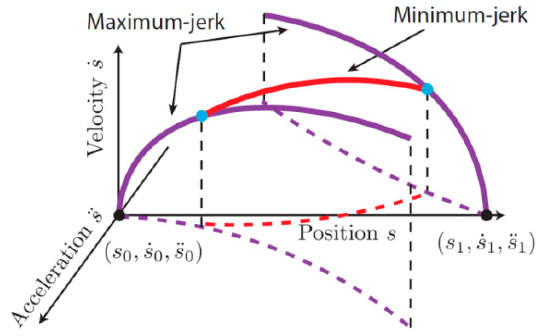
Most of these methods are based on the optimal control theory. By determining the maximum acceleration/deceleration on the path, and then integrating the calculation speed curve, the time-optimal trajectory is obtained. However, the key aspect of this method is to find the conversion point between the acceleration section and the deceleration section, and the acceleration curve is converted between the maximum acceleration and the maximum deceleration before and after the conversion point. The time-optimal trajectory method includes velocity, acceleration and torque constraints, but the process of finding the transition point is complex, and the stability is poor. The TOPP method is proposed based on the TOTG method, which further improves the method of finding the conversion point and reduces the computational complexity. However, the above two methods ignore the acceleration constraint, which leads to the problem of acceleration mutation in the time-optimal trajectory. In the follow-up work, the acceleration and torque rate constraints are introduced into the numerical integration method to obtain a smooth-running time-optimal trajectory, but the method to find the conversion point is not complete and cannot find all the conversion points (Figure 1).

3.4. Convex Optimization Method

The method discussed herein continues to follow the optimal control theory. It determines the maximum acceleration and deceleration on the path based on convex optimization and then integrates these factors to calculate the speed curve. With the flexibility to set optimization objectives, this method can address multi-objective optimal trajectories—such as time, energy, stability—and offers a calculation speed faster than other methods.

One such solution is a time-optimal trajectory planning method based on convex optimization. This technique can find the transition point faster and easier than other methods such as TOTG and TOPP. However, it does not consider acceleration constraints, resulting in sudden acceleration changes in the trajectory. These changes can negatively affect the stability of the trajectory execution.

To address this, the jerk constraint is approximated as a linear function and is introduced into the convex optimization problem. This adjustment aims to achieve a smooth time-optimal trajectory. Even though this method preserves the convexity of the optimization problem, it adds to the number of optimization variables, leading to a significant increase in computing time.

In seeking to optimize both time and acceleration, another method employed is a non-dominated sorting genetic algorithm. This algorithm allows for a smooth time-optimal trajectory. However, it does not consider the torque constraint.

In conclusion, directly introducing the acceleration constraint into the convex optimization problem destroys the convexity of the problem, increasing both the number of optimization variables and calculation time. Nonetheless, compared to dynamic programming and numerical integration methods, the convex optimization method is simpler and more stable. It delivers a faster calculation speed when the optimization variables are fewer. For the same time-optimal trajectory planning problem, the calculation time of the dynamic programming method is 8.5 times that of the convex optimization method, and the numerical integration method is 15.3 times that of the convex optimization method.

Despite these benefits, it is important to note that convex optimization methods have not yet been widely accepted for handling nonlinear acceleration constraints. This remains a challenge to be addressed in further research and development in the field.

3.5. Algorithm Based on Machine Learning

Just as the world’s major robot companies are committed to developing intelligent sorting robots, the research on robot sorting methods is also a hot issue for many researchers. To better understand how this is achieved, it is crucial to delve into the technical aspects of intelligent sorting robots. In this setup, the image of the robot’s current working scene is semantically segmented. The position and posture of the object in the image, as well as the category of the object, are identified. This semantically segmented image is then input into the deep neural network. By using a reinforcement learning algorithm, the deep neural network is trained to output the correct robot action command, which completes the desktop item sorting task.

Building on previous work, this sorting method is expanded to propose a general paradigm for object sorting tasks. Nicola discretized the robot’s working environment into 3D grids, where the state of each grid represents the semantic attributes, such as the category and order of the objects in the grid. Without changing the framework of the sorting model, the deep reinforcement learning algorithm trains the robot sorting model to solve different classification tasks. Addressing environmental factors such as light changes that make manual feature extraction impossible, the hierarchical extreme learning machine is used. In the absence of output labels for this task, the reinforcement learning algorithm trains the sorting strategy. The proposed HELM-RL method shows strong robustness to changes in the external environment and high accuracy for each sorting task. Furthermore, a learning algorithm based on the Distinguished Node (DN) is utilized to create a feasibility distribution map of object sorting, which guides the generation of the best sorting action. The deep deterministic policy gradient algorithm is used to train the robot’s throwing strategy. This results in an output of the throwing speed of the robot’s end effector, enhancing its working ability and efficiency in the weak structure logistics sorting scene.

In addition to these learning algorithms, other data types like RGB-D are also crucial in the sorting process. The RGB-D data are used as the input of the convolutional neural network to identify the object to be grasped by the robot and determine the corresponding point cloud cluster. A grasping generator algorithm is then used to output potential grasping actions from the selected point cloud data, which are scored by the grasping filter. The highest scoring grasping action will be used for robot execution.

Once the robot has grasped an object, further algorithms, such as the HVS mode, are applied to sort the objects. Using the HVS mode algorithm, a sorting robot system for classifying objects of different colors and identifying object positions is established. The system can sort objects to the appropriate conveyor belt in real time based on their color. It can also identify the shape of objects, picking out all objects of the same shape and placing them on the corresponding conveyor belt.

4. The Stability Prediction Model of Manipulator Based on LSTM-XGboost

In recent years, deep learning algorithms have been widely used in the field of robotic arms. With the popularity of intelligence, more and more robotic arms come into contact with the environment to perform complex and dangerous tasks. When the external environment contact force is generated, the safety and flexibility of the manipulator are very important. A variety of impedance control strategies are designed from the perspective of control. For example, Reference adopted a position-based adaptive impedance control method for the grinding robot, effectively tracking the end’s ideal position and solving the grinding trajectory’s compensation correction problem. For the lower-limb rehabilitation robot based on impedance control, the human–machine interaction torque is set as the constraint condition for real-time control. The parameters of the end impedance model of the robot are adjusted online to make the robot adapt to the external environment to realize the robot’s compliant control.

The manipulator is a complex multi-input multi-output system. In actual control, the dynamic model and joint friction of the manipulator are unknown in most cases, affecting impedance control’s robustness. In order to improve the compliance control effect of the manipulator, this chapter proposes a stability prediction model of the manipulator based on LSTM-XGboost.

4.1. XGboost Method

XGboost is an abbreviation of extreme gradient boosting, which is often used to solve classification or regression problems in engineering. The Boosting method is a commonly used statistical learning method, and Boosting Tree is a high-performance ensemble learning method. The classification tree or regression tree is used as the basic classifier, and the linear combination of the forward distribution algorithm and the tree is used. By changing the weight of the training samples, multiple basic classifiers are learned and linearly combined to continuously improve the performance of the model.

$$f_M(x)=\sum _{m=1}^{M}T\left(x;{\mathsf{\Theta }}_m\right)$$

(7)

$$T\left(x;{\mathsf{\Theta }}_m\right)=\sum _{j=1}^J{C}_{j}I\left(x\in R_j\right)$$

(8)

Among them, T(x; Θ_m) represents the decision tree, Θ_m is the parameter, M is the number of trees; j represents the number of disjoint regions that divide the input space, and C_j represents the output constant for each region.

4.2. LSTM Method

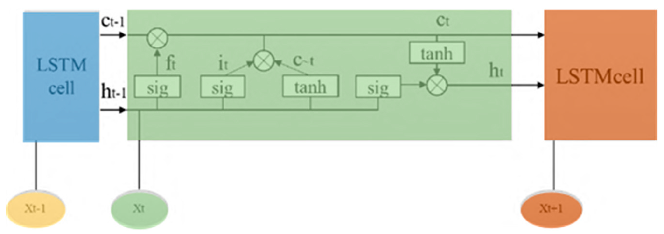
Long short-term memory network (LSTM) is a variant of recurrent neural network (RNN). It is composed of a series of neurons and is often used to learn sequence signals with information transmission. The coefficient matrix of each neuron is shared; that is, their values are the same, and the control gate and memory unit are introduced inside the neuron. The coefficient of the LSTM in a single neuron is about 4 times that of an RNN neuron, where it is the input gate that controls the amount of new information stored in the new memory unit c~t to the current memory unit c_t; ft is the forgetting gate, which controls the amount of information retained in c_t−1 at time t − 1; o_t is the forgetting gate, which controls the amount of information transmitted to the hidden state h_t in the current memory unit c_t; and h_t is the hidden state and also the output of each neuron of the LSTM, as show in Figure 2.

4.3. Based on LSTM-XGboost Prediction Model Construction

The most common solution to the optimal trajectory planning problem of the manipulator is to discretize the trajectory into a finite number of path points. At each path point, according to the motion state of the manipulator, the optimization variable is taken as a positive maximum or a negative maximum within the allowable range, which is the so-called optimal control theory. The optimal control theory is shown in the time-optimal trajectory planning problem of the manipulator. Under the kinematic and dynamic constraints, the maximum acceleration or maximum deceleration is selected at each path point to maximize the speed, thereby optimizing the running time of the trajectory. The running stability is manifested as the acceleration constraint in the time-optimal trajectory planning problem of the manipulator. By limiting the change rate of acceleration, the trajectory can run smoothly. The acceleration constraint usually appears in the form of a third-order Lagrange dynamic equation, but the equation is nonlinear and difficult to deal with in the optimization process, so the acceleration constraint is usually ignored in the time-optimal trajectory planning of a manipulator. However, ignoring the jerk constraint will make the acceleration mutation problem easy to occur in the planned trajectory, aggravate the vibration of the end of the manipulator, and even cause the trajectory to be unable to execute on the manipulator. Therefore, it is of great significance to properly solve the nonlinear acceleration constraint for the time-optimal trajectory planning problem of the manipulator with running stability constraint.

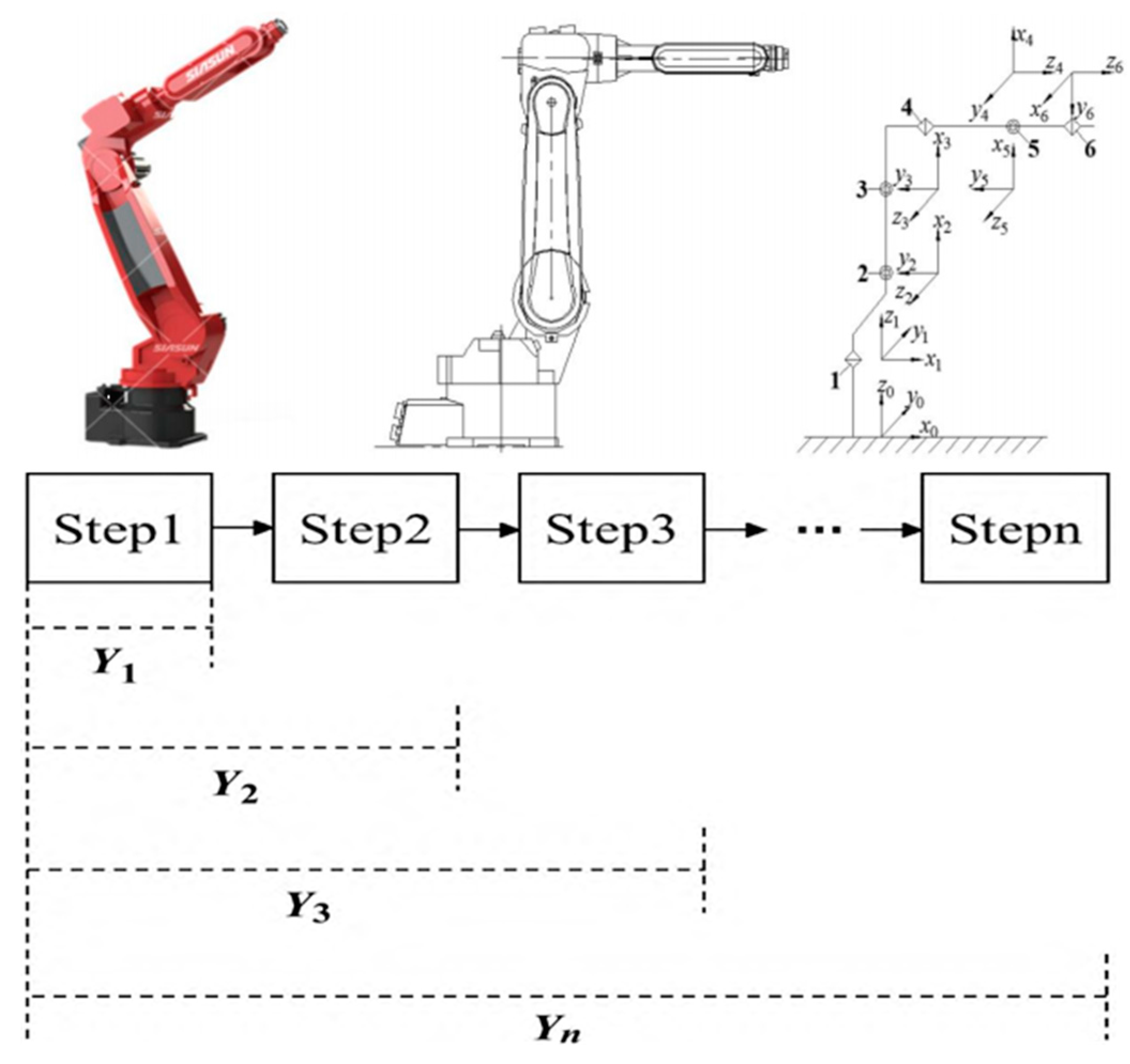
In actual control, the dynamic model and the joint friction of the manipulator are often not accurately obtained, which poses a challenge to the trajectory tracking control accuracy of the manipulator. The high-speed smooth-motion trajectory planning of a multi-axis serial manipulator based on optimal control theory is used to calculate the maximum acceleration or maximum deceleration under acceleration and other constraints, so as to maximize the speed. However, the speed of a high-speed smooth trajectory does not always increase or decrease, but rather frequently changes between acceleration and deceleration. Therefore, in order to calculate the maximum velocity curve under acceleration and other constraints, it is very important to find the conversion point between the maximum acceleration and the maximum deceleration of the high-speed smooth motion trajectory. Before finding the conversion point between the maximum acceleration and the maximum deceleration, it is necessary to determine the feasible velocity curve corresponding to the given path. In order to make the starting point speed and the end point speed of the feasible speed curve equal to the preset starting point speed and the end point speed of the given path, the maximum speed curve needs to be calculated forward and backward, respectively. In the calculation of the forward maximum speed curve, the XGboost algorithm is used to construct the ‘instruction-feature index’ prediction model. The model input is the instruction parameters of the manipulator, including speed v, acceleration a, displacement D, and the output index of the previous step; the output is the current sequence segment index. The stability index of the manipulator is denoted as Y; Y is the vector value, namely Y = (|a|_ave, δ_a, a_p, δ_w, jerk). When predicting it, the continuous motion of the manipulator is first decomposed into n single-step motions according to the action. The decomposition diagram is shown in Figure 3.

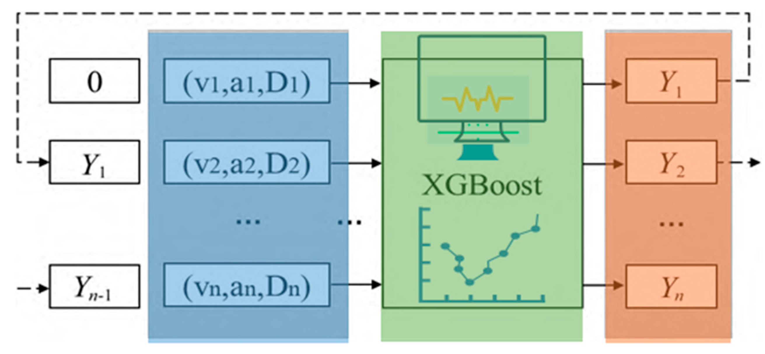
The instruction-feature index prediction process based on XGboost is shown in Figure 4. After each single step of movement, the velocity v, acceleration a and displacement D are input into the XGboost model together with the Y value of the previous step, and the cycle is repeated until the end of the action and the resulting Y_n is the final feature index.

The vibration signal of the manipulator is collected by the six-axis Bluetooth attitude angle measurement sensor, and the sampling frequency is 100 Hz. The measurement sensor is fixed at the end of the six-axis manipulator. The collected signals include the acceleration, angular velocity, and angle of the XYZ axis in the tool coordinate system of the six-axis manipulator. The sample size of the test set in the data set is 300, and the ‘instruction-feature index’ model built in this chapter is used to predict Y. Considering that the five indexes have the same order of magnitude, the accuracy is measured by the mean absolute error (MAE). According to the above process, the model is established, and the motion sample of the manipulator is divided according to the action; that is, the input instruction for each action and the prediction information of the previous action are input, and the output is the overall indicator jerk of the sample until the action. During training, Steps are set to the number of actions of each sample, and Loss is the root mean square of the error of the entire moving process so that the complete sample motion process can be gradient descent. The number of iterations is set to 1000, and the learning rate is 0.1. Taking jerk as an example, the model predicts the jerk of a single action index. It can be seen that the model performs well in the prediction of the action index, and the error is 0.0005. See Figure 5.

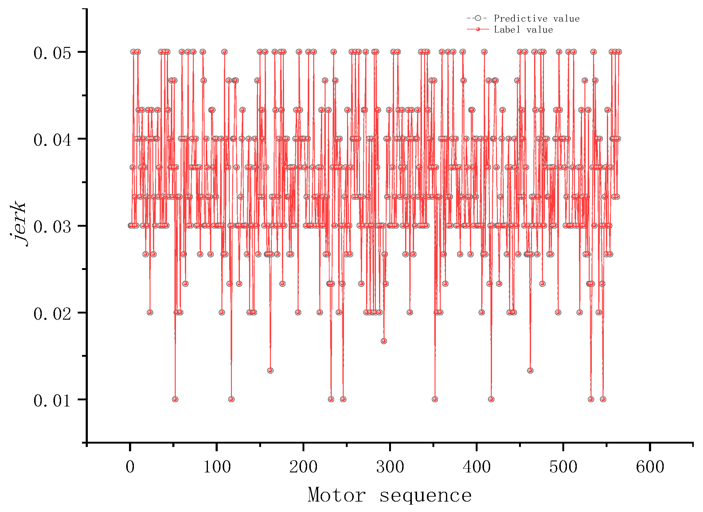
Further observation of the model’s performance on the full sample motion shows each sample, including multiple actions and multiple instructions. According to the instruction combination sequence, the index jerk of the sample is predicted. Figure 6 shows that the model can give the sample motion index jerk according to the instruction sequence, and the consistency is good. The performance of the model in index prediction is shown in

Table 2. Evaluation of Model Prediction Effect.

Type	MAE
$|a{|}_{ave}$	0.0032
δa	0.0024
ap	0.0027
δw	0.4721
jerk	0.0051

. It can be seen from the results in Table 2 that the MAE values predicted for the five indicators are low and the prediction accuracy is high.

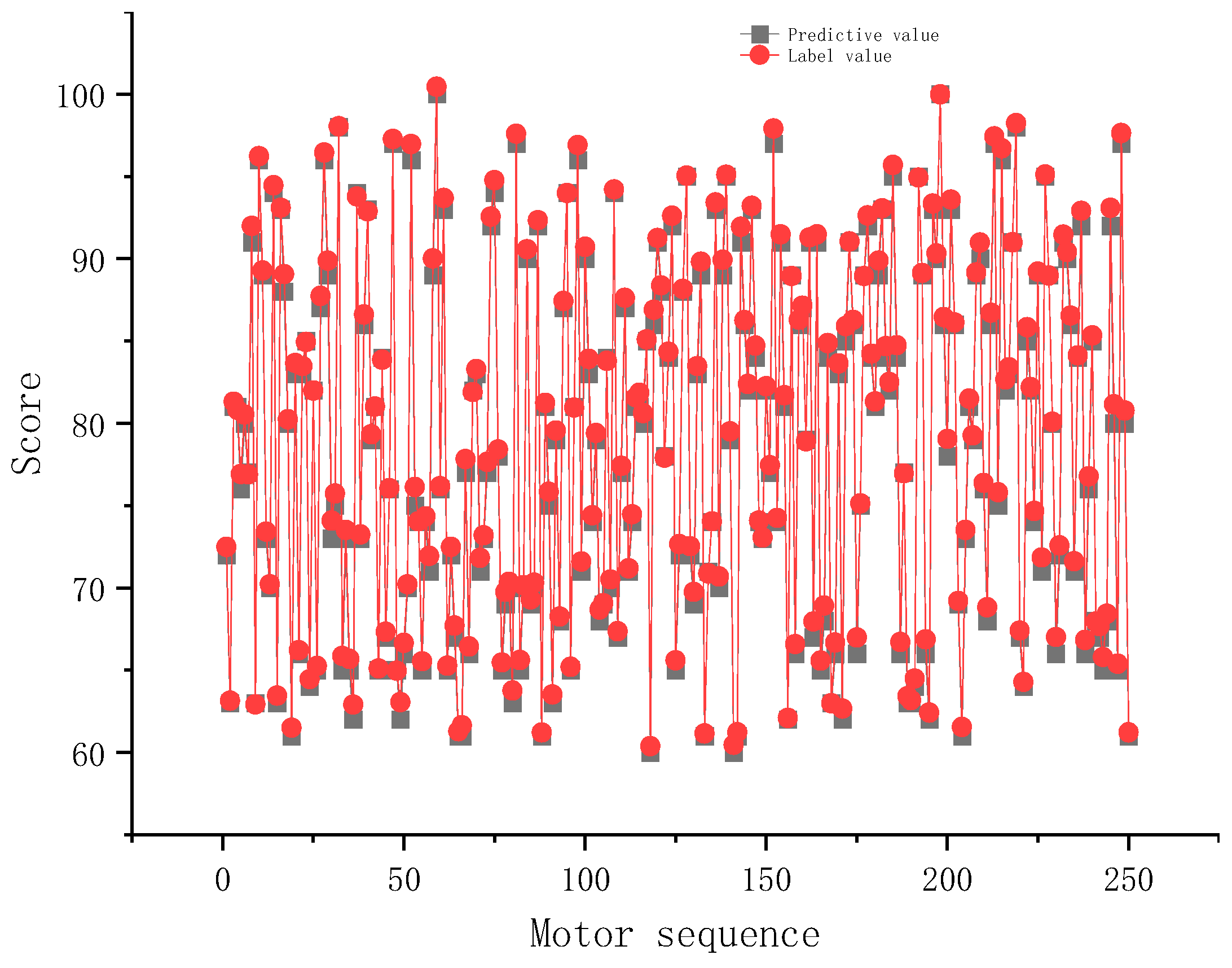
The feature indicators and input instructions obtained in the XGboost model are used as the input of the LSTM model, and the score card is scored as the label value. The model is trained, and the output score prediction value of the LSTM is compared with the sample score card score.

From Figure 6, we can see that the prediction score transformed from the prediction stability index is roughly consistent with the actual score card score, and the absolute mean score error is 2.06 points, which is due to the influence of model error. Overall, the prediction effect of the stationary prediction model is better.

5. Discussion

In the field of manipulator control, achieving efficient, safe, and stable motion control remains a continuous challenge, especially when addressing complex tasks and environments that require accurate trajectory prediction and control. A novel solution is presented in the form of a hybrid machine learning model based on LSTM and XGBoost, which aims to predict the motion stability of the manipulator. The inclusion of LSTM enables effective modeling of time-dependent characteristics in the data, while XGBoost’s incorporation allows for capturing complex non-linear relationships. The combination of these methods enhances prediction performance.

The model is trained on actual motion data from the manipulator, including parameters such as speed, acceleration, and displacement. This data-driven training approach bolsters the model’s applicability in real-world scenarios and its generalization capability. Training results reveal that the prediction error for a single-action index is minimal, demonstrating impressive prediction prowess.

The model’s performance was evaluated not only on individual action indices, but also on complete motion sequences. Given a series of command sequences, the model can provide the motion index for a sample, showing consistency. Furthermore, the low average absolute error of the five indicators suggests high prediction accuracy.

However, despite its overall effective prediction capability, some discrepancies have been observed between the model’s score predictions and the actual scores. These discrepancies likely arise from inherent model errors, suggesting potential avenues for further optimization to enhance prediction accuracy.

In conclusion, the manipulator stability prediction model based on LSTM-XGBoost provides a new and effective method for predicting and controlling the motion state of robot arms. Future work aimed at refining this model could hold significant promise for the broader applicability and optimization of robotic arm control.

6. Conclusions

In this study, by analyzing the relationship between the command parameters of the robotic arm and the motion stability, the command-feature index and feature index-stability score prediction models are established by using XGBoost and weight-sharing LSTM models to predict the motion performance and stability of the robotic arm with high accuracy so as to meet its operational stability and time optimality requirements under the ever-increasing motion performance requirements and labor cost pressures. The main conclusions are as follows:

(1)

By using the six-axis Bluetooth attitude angle measurement sensor to collect the vibration signal of the manipulator, and using the XGboost model and the weight-sharing LSTM model, the command-characteristic index prediction model and the characteristic index-stability scoring model are established. These models can predict the acceleration, angular velocity and angle on the XYZ axis during the movement, as well as the overall performance indicators of the robotic arm, such as jerk. The performance on training and test sets is good, the mean absolute error (MAE) is low, and the prediction accuracy is high.

(2)

The model can handle complete sample motions containing multiple actions and multiple instructions. According to the instruction combination sequence, the model can predict the immediacy index of the sample, and the consistency is good. In addition, according to the predicted stability index, the model can convert and predict the predicted scores that are roughly consistent with the sample score card scores, although there is an absolute average score error caused by the model error.

(3)

With the increase of labor costs year by year, the mechanical arm has replaced the repeated labor of people in more and more positions, but this also puts forward higher requirements for the motion performance of the mechanical arm. Operation stability and time optimality are two of the most important requirements for the motion performance of manipulators. Researchers usually calculate the maximum velocity curve that satisfies the acceleration constraint by transforming the operational stability requirement into the acceleration constraint so as to obtain the time-optimal trajectory of the manipulator with the operational stability constraint. The above model shows good performance in this aspect and can predict the corresponding stability score according to the set parameters so as to effectively optimize the operation performance and stability of the manipulator.