1. Introduction
The decision-making process is highly intricate and involves cognitive and emotional aspects [
1]. Before making a choice, the brain evaluates various options and their potential outcomes. However, in an unpredictable world, the brain also owns the capacity to cancel impending actions. Past experiences, emotions, social context, and personal values are among factors that influence decision making [
1,
2].
Neuroscientists use electroencephalography (EEG) to measure brain activity and find the neural correlates of the decision-making process. EEG can be used by researchers to examine how the brain reacts to various options and pinpoint the variables that affect decision making. EEG-based brain–computer interfaces (BCIs) can be used to measure how people react emotionally to various stimuli, such as pictures or videos. Decision-making BCIs have various benefits, including faster response times, improved correction of mistakes, and enhanced independent learning [
3].
BCI can be classified as active or passive in terms of human control over the machine. The active BCI devices collect users’ brain signals activated intentionally with user consciousness to provide human control over equipment using event-related potentials (ERP), for example, using collaborative BCI for better-coordinated group decisions in a Go/NoGo task using EEG [
4]. Passive BCI devices, on the other hand, collect users’ brain signals triggered unintentionally and without the users’ consciousness to study users’ emotions outputted involuntarily as a result of the effect of a surrounding environment [
5]. This can be used to identify the true choices and obtain hidden information in users’ brains about their actual thoughts, choices, and decisions.
During the decision-making procedure, the human brain gathers and incorporates all sources of previous evidence and values to yield a choice. Based on such information, the decision maker gains an assessment of the probability of the decision being correct i.e., confidence. BCI can be used to predict the decision confidence from EEG using two classes ‘confident’ and ‘non-confident’ [
6]. BCIs are able to identify alterations in brain activity linked to either positive or negative emotions, giving them insight into a person’s preferences [
7].
Artificial intelligence (AI) research can develop more accurate prediction models of individuals’ behavior and preferences by understanding the neural mechanisms underlying decision making and emotional responses. By utilizing AI and deep learning (DL) models, it is possible to extract meaningful patterns and insights from large datasets, which can then be used to enhance services and applications in different contexts.
This research aims to build an individual choice prediction system using EEG signals. The SJTU emotion and EEG dataset (SEED) is a benchmark dataset used in this research to investigate individuals’ hidden information about actual choices using EEG signals [
8]. EEG is a practical, flexible, and affordable technique. It provides a high temporal but low spatial resolution measurement of brain activity [
9], which has been widely used for various purposes, including the analysis of reactions to emotional stimuli.
In this paper, we build different DL models, such as a convolutional neural network (CNN), long short-term memory (LSTM), and a hybrid model. We also compared their performance with different classical classifiers, such as k-nearest neighbors (KNN), support vector machine (SVM), and logistic regression (LR). We also utilized ensemble classifiers, such as random forest (RF), adaptive boosting (AdaBoost), and extreme gradient boosting (XGBoost). We evaluated our proposed models and compared them with previous studies using SEED.
This paper is organized as follows:
Section 2 presents the background;
Section 3 illustrates the literature review;
Section 4 explains the research methods and BCI framework;
Section 5 explains the experiment implementation;
Section 6 discusses the results and the comparison of classical classifiers with related studies; and
Section 7 presents the conclusion and future works.
2. Background
In this section, we first explain the techniques used in signal processing, followed by a description of the classification algorithms used. Finally, related works that used the benchmark dataset are discussed.
2.1. Signal Processing
Signal processing is an essential step for choice classification, which includes two steps: signal preprocessing and feature extraction.
First, EEG signals are preprocessed to remove artifacts from the recorded signals and enhance the ratio of the signal power to the noise power. EEG artifacts result from either physiological or technical factors. Physiological artifacts are the signals generated by movements of the physical parts of the body, such as the head, face, neck, and eyes. The technical artifacts are related to powerline noises and electrode resistance variations. Since the EEG signals are noninvasive and the power lines cannot meet with the signals being collected, this generates a low signal-to-noise ratio [
10].
Next, feature extraction is applied after the preprocessing to reduce the high dimensionality of the EEG data [
10]. EEG signals can be analyzed in terms of two domains: frequency and time [
11]. To extract relevant features for choice prediction, frequency domain analysis was employed in this study since it is the most commonly used approach in neuromarketing studies [
12].
2.2. Classification Algorithms
In computer science, DL is one of the machine learning (ML) methods that is based on the artificial neural network (ANN). ANN, otherwise known as a neural network (NN), can be used for supervised ML and is one of the recommended models because it can recognize patterns and handle common problems by reflecting the behavior of the human brain consisting of its simplest architecture (perceptron).
However, DL architecture, sometimes called a deep neural network (DNN), uses more than two hidden NN layers consisting of multi-layered perceptrons. DL has a strong ability to solve image recognition, speech recognition, natural language processing problems [
13], image reconstruction [
14,
15], and biomedical imaging [
16]. It has also been effectively employed in the field of BCI for classifying EEG motor imagery signals and detecting emotions through EEG [
5].
One of the main DL models is the CNN, which is derived from the visual cortex of animals. The data input to a CNN model is first divided into different neural fields to be fed into one- (ID) or two-dimensional convulsion layers [
17,
18].
Another DL model is the recurrent neural network (RNN), which is characterized by its “memory.” It takes the information from previous inputs to influence the current input and output. While traditional DNN assumes that inputs and outputs are independent of each other, the output of the RNN depends on the sequence of prior elements [
19].
The LSTM model is a subtype of the RNN. It has a feature through which it can memorize the sequence of the data. Thus, it is capable of learning long-term dependencies, which overcomes the issue of gradient disappearance. It is also useful for eliminating unused information. The LSTM network is parametrized by weight matrices from the input and the previous state for each of the gates [
19].
A hybrid model combining CNN and LSTM is an approach where the strengths of both architectures are utilized in solving complex problems. Such a model offers the advantages of CNN’s capability to learn spatial hierarchies and capture local features, along with LSTM’s capacity to learn long-range temporal dependencies and manage sequences. The hybrid model architecture can vary depending on the specific problem being addressed. The choice between starting with CNN followed by LSTM or LSTM followed by CNN mainly depends on the task and the nature of the input data.
The KNN algorithm is a simple, easy-to-implement supervised ML algorithm that can be used to solve both classification and regression problems. It works by classifying instances based on the similarity between them to locate the nearest neighbor. The new labeled sample will be put up against the benchmark data for comparison by the choice classification. Based on the class that the majority of KNNs belong to, the voting formula will decide where the new labeled sample will be allocated [
10].
SVM is also among the most widely used supervised ML algorithms for both classification and regression problems. The fundamental concept behind SVM is to use a kernel transfer function to project incoming data onto a higher-dimensional feature space that is simpler to separate than the initial feature space [
20].
LR is a supervised ML that has been widely employed in ML for EEG signal processing [
21]. We employed LR, whose output value corresponds to the probability of belonging to a choice class.
Ensemble models can combine many weak learners into a strong learner. RF is an ensemble-learning algorithm that uses a collection of random decision trees trained via the bagging method [
22,
23]. It works by adding randomness to the tree training process and merging the results of various randomized trees into a singular classifier. The final result is a tree with decisional nodes and leaf nodes that indicate the choice class.
In addition, two more ensemble-learning algorithms have been utilized in this study via the boosting method. We used AdaBoost, which is an adaptive enhancement algorithm for binary classification. The new predictor in AdaBoost pays a little more attention to the training instances where the predecessor is misclassified [
24].
The last ensemble in this study is XGBoost, which is an optimized implementation of gradient boosting available in the Python library [
25]. It is based on the iterative fitting of residuals resulting from the subsequent training and predictions generated by weak learner algorithms [
25,
26]. The final choice class with a higher probability result from the ensemble of decision trees that meets on small residuals or when the maximum number of trees is reached.
3. Related Works
In recent years, there has been an increasing interest in utilizing EEG signals for emotion recognition and prediction for human reactions based on their responses to emotional stimuli. Several studies have explored the use of DL models to develop accurate emotion recognition systems using EEG signals.
One such study by Zheng and Lu [
8] introduced the use of deep belief networks (DBNs) for constructing EEG-based emotion recognition models from 62 channels for three types of emotions: positive, neutral, and negative. They extracted five features: power spectral density (PSD), differential entropy (DE), differential asymmetry, rational asymmetry, and the differences between the DE features of 23 pairs of frontal–posterior electrodes. A comparison between DBN and the shallow models (SVM, LR, and KNN) was conducted, with the average accuracies being 86.08%, 83.99%, 82.70%, and 72.60%, respectively. They also proposed a DBN-based method for selecting critical channels and frequency bands using the weight distributions of the trained DBNs. Among the different electrode sets, 12 channels with SVM achieved the highest accuracy (86.65%) and lowest standard deviation (8.62%), surpassing the accuracy of the 62 channels with SVM (83.99%) and DBNs (86.08%).
Asghar et al. [
27] extracted features using the discrete wavelet transformation method and the AlexNet model from 62 channels in SEED. They used the bag of deep features as a dimensionality reduction and attained 93.8% accuracy with the SVM classifier.
Lu et al. [
28] extracted features using dynamic sample entropy measures from all channels over time. They utilized SVM and achieved an average accuracy of 85.11% for identifying negative and positive emotions. Bai et al. [
29] chose eight channels to classify positive and negative emotional states. They used the wavelet transform (WT) approach to decompose and extract the frequency band and calculate the sample entropy. They proposed LSTM and achieved a final accuracy rate of 90.12%.
4. Methods
The main objective of this research is to provide a framework and build a system for detecting individuals’ preferences and choices based on the options presented to them using EEG-based BCI. The motivation for our research work lies in the fact that decision making has an unconscious and direct component that may drive or affect overt preferences and actual choices.
Consequently, we aim to identify the main relevant features in the EEG signals of individuals and determine the attributes that contribute to a better understanding of how individuals perceive images and videos that affect their decisions. In this section, we explain the general BCI framework and discuss the neural correlates of choices in EEG signals.
4.1. General BCI Framework
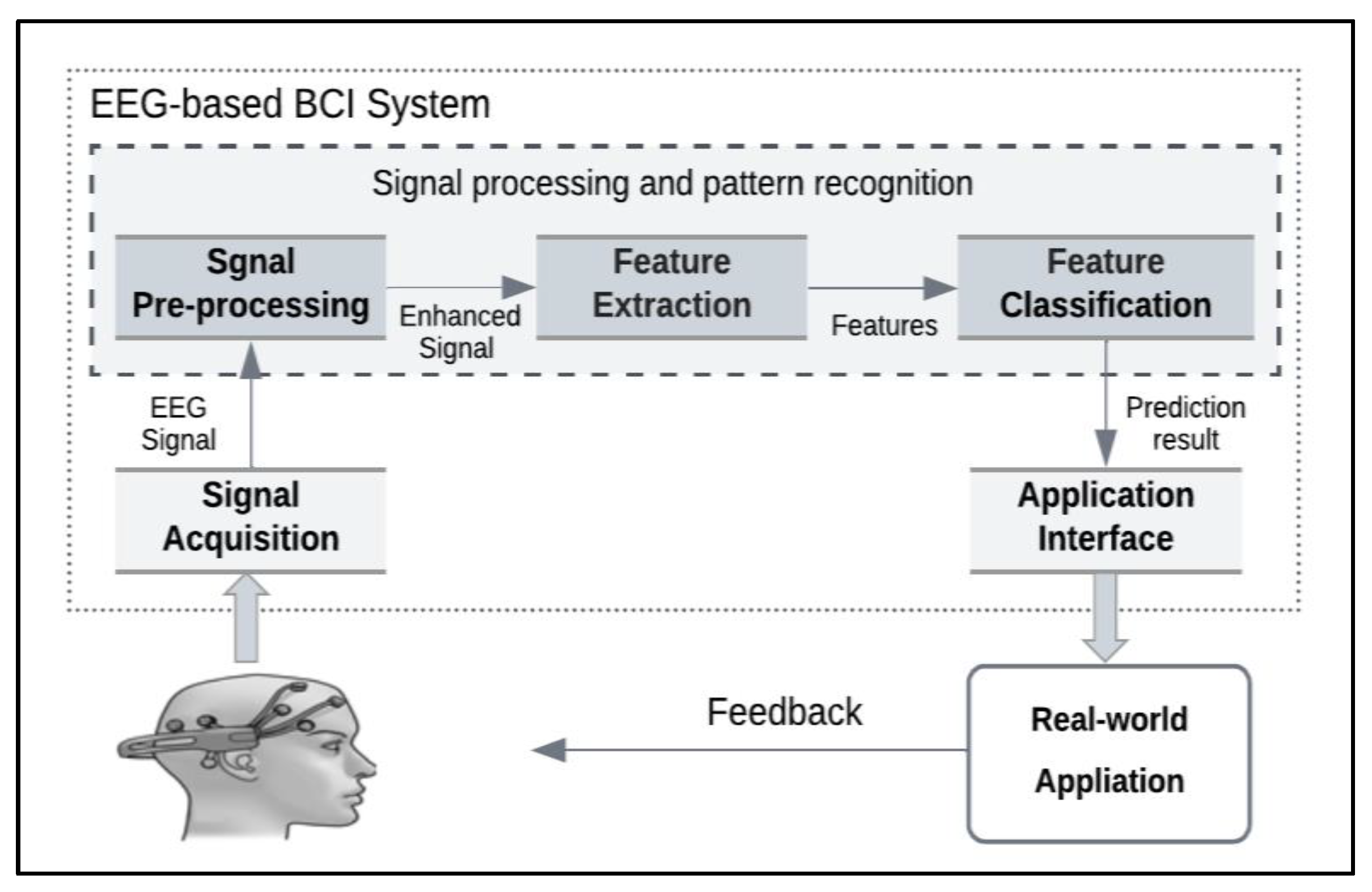
We measured EEG signals using a BCI device, which is human–machine communication. Thus, the generic BCI framework (
Figure 1) is based on the three core components: the signal acquisition stage, the pattern recognition stage, and the application interface stage.
In the signal acquisition stage, brain signals are measured using a specific type of sensing modality (EEG, fNIRS, MEG, etc.). Then, the recorded signals are fed into the signal processing stage for ML and pattern recognition.
The pattern recognition stage includes three steps: preprocessing, feature extraction, and classification:
- a.
In the signal preprocessing stage, any noise from the signals is filtered and removed to best digitize them for the computer.
- b.
Relevant characteristics of the signals are extracted in the feature extraction stage.
- c.
In the classification stage, extracted features are analyzed and translated to an output using ML.
The application interface stage presents the classification results to the user and performs the proper action based on the BCI application.
4.2. Neural Correlations of Choices
We designed and developed our choice detection system based on the four main choice indices found in the literature [
30]: approach–withdrawal (AW) index, valence index, effort index, and choice index.
The AW index is the frontal asymmetry between the left and right hemispheres. The left hemisphere indicates higher activation of positive emotions, while the right hemisphere indicates higher activation of negative emotions. The frontal asymmetry theory of brain activity is found in [
11].
The valence index is based on the Russell emotional model for the valence dimension [
31]. A high valence represents a “like” choice state, whereas a low valence represents a “dislike” choice state. Research has proven the relationship between the asymmetry of frontal activation and the valence of a person’s emotions.
The effort index computes the difference in the theta frequency band in both the left and right frontal hemispheres, with a larger value representing a greater load and effort in the working memory [
32].
The choice index measures the alteration of the beta and gamma frequency bands in both frontal hemispheres, with a higher value representing a greater possibility of making a choice [
33].
5. Experiment Implementation
In this paper, we build the choice prediction model using the SEED benchmark dataset. Therefore, a description of SEED is provided. Our proposed EEG-based BCI system for individual choice detection consists of four key modules: preprocessing, feature extraction, feature calculation, and choice classification using DL. Each module is detailed in
Section 5.2,
Section 5.3,
Section 5.4 and
Section 5.5.
For model evaluation, we assessed our choice classification model in terms of three measures: accuracy, precision, and recall. We also compared its performance with different classical classifiers such as KNN, SVM, and LR. We also utilized ensemble classifiers such as RF, AdaBoost, and XGBoost.
For the system implementation, we used an open-source programming language, i.e., Python, and the Scikit-Learn toolbox for ML, along with SciPy for EEG filtering and preprocessing, MNE for EEG-specific signal processing, and the Keras library for DL. We subscribed to Google Colab Pro+ in order to have high memory for running our DL model.
5.1. Dataset Description
One of our main challenges in this research was the lack of EEG emotional benchmark datasets. However, there are some publicly available EEG emotional benchmark datasets used in neuromarketing research, such as the DEAP dataset [
34], the neuromarketing dataset [
35], and SEED [
36].
In this paper, we used SEED to train the model of the proposed system. EEG datasets were provided by the brain-like computing and machine intelligence laboratory, Shanghai Jiao Tong University. The SEED dataset has been used to conduct multiple studies and has been proven to be well-suited for testing new algorithms [
8,
27,
28,
29]. These studies have demonstrated the effectiveness of various ML techniques, including deep learning approaches, in classifying emotional states using the SEED dataset.
Table 1 summarizes some information about SEED.
SEED contains EEG signal recordings of 15 Chinese participants (7 males and 8 females) that were collected with 62 channels. Their emotions during the recording were triggered using 15 Chinese film clips containing positive, neutral, and negative emotions. The video clips (stimuli) were selected with specific criteria: (1) each video clip includes only one targeted emotion; (2) the video content is clear and can be understood without descriptions; and (3) each experiment has an appropriate duration to avoid subjects experiencing fatigue.
In SEED, each participant completed the experiment through three different sessions with a time interval of about one week to ensure the stability of reading signals. Each session contained fifteen different video clips, and their presentations were ordered in such a way that two clips did not trigger the same emotion consecutively. There was a 5 s hint at the start before each video clip, followed by the 4 min video clip presentation and a 45 s self-assessment questionnaire to report the immediate emotional reactions to each video clip. A 15 s rest is provided afterward. Each video clip was linked into one emotion: positive, negative, and neutral labeled as 1, −1, and 0, respectively.
5.2. Preprocessing
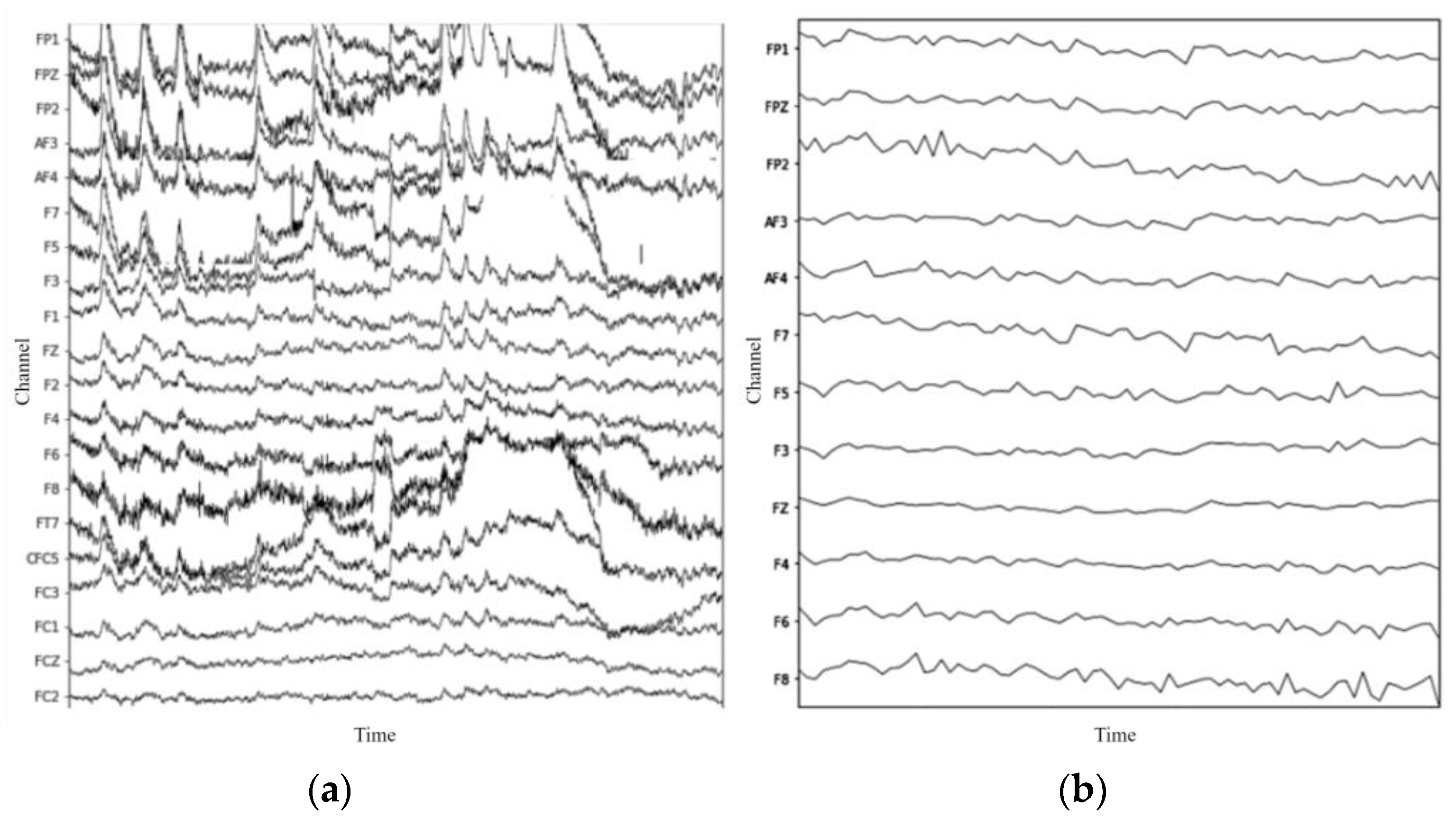
Preprocessing techniques were applied to SEED to improve the quality of the EEG signals. Electromyography (EMG) and electrooculographic (EOG) artifacts were removed manually.
The signals were downsampled to 200 Hz, and a bandpass frequency filter was applied between 0.5 Hz and 75 Hz, which contains the EEG information and discards the noise from the signals.
In addition, we applied more preprocessing steps, which are discussed below.
Figure 2 represents some of the EEG data before and after preprocessing.
- (1)
Since frontal brain areas are correlated with an individual’s choice state [
37], we picked 12 related channels for detecting induced choices. The 12 channels were selected based on the guidelines provided in reference [
37], which recommends the selection of channels that have been shown to be reliable and informative in previous studies. Specifically, these channels were chosen based on their relevance to measuring emotional responses and have been used in previous studies on emotion recognition using EEG signals. The selected channels include FP1, FPZ, FP2, AF3, AF4, FZ, F3, F4, F8, F7, F5, and F6.
- (2)
Because emotions may not be triggered at the beginning of each trial, we discarded the first 60 s and cropped the time to obtain 1 min long EEG data.
- (3)
We further applied a bandpass filter between 1 Hz and 50 Hz.
5.3. Feature Extraction
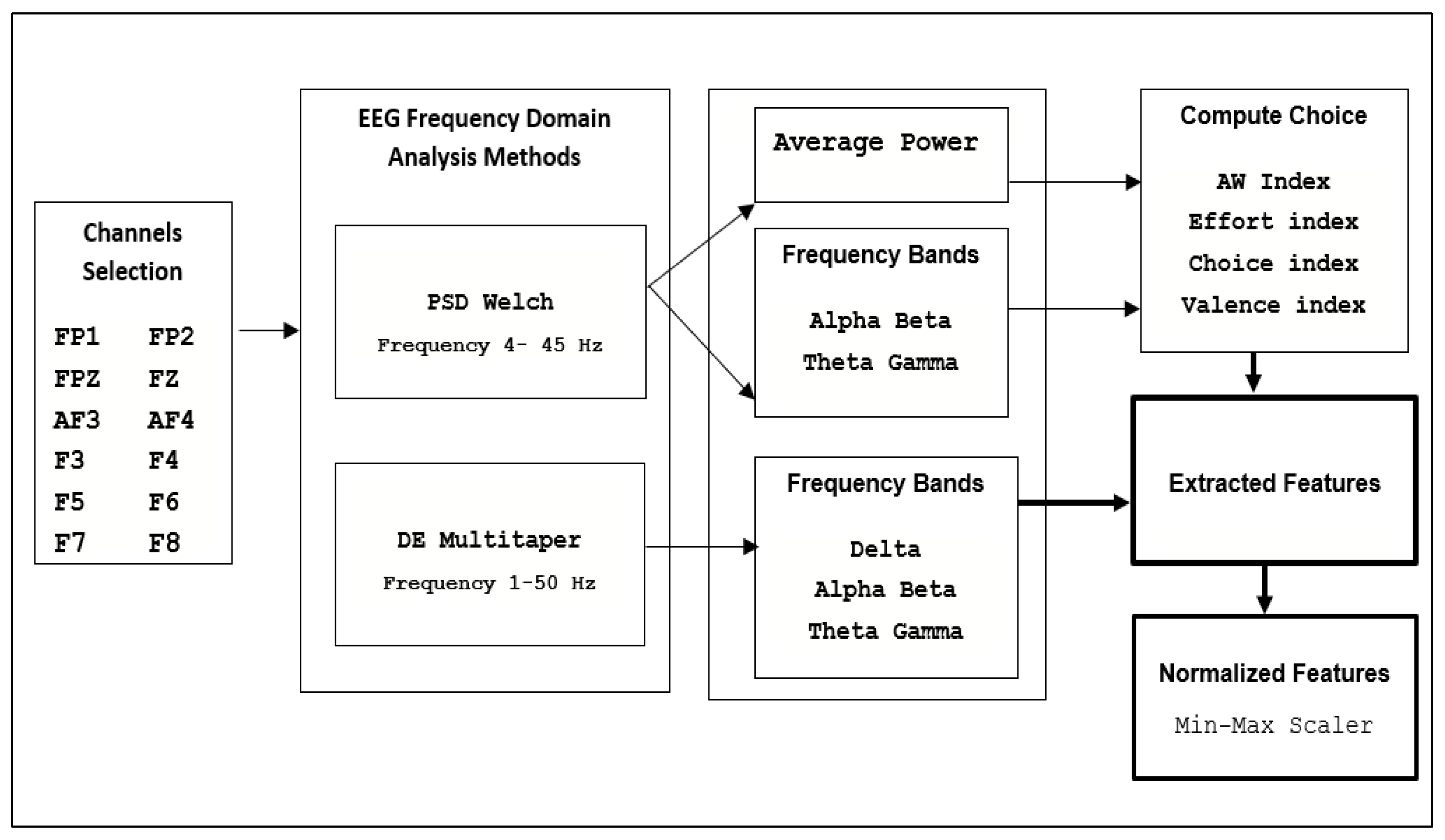
First, we divided the EEG signals into a fixed length of 1 s using the Hanning window without overlapping. Then, we extracted the EEG features using frequency-based analysis, the PSD, and the DE.
The PSD technique is based on the Shannon entropy of the power spectrum and the Welch method. We used PSD to extract the average power features into four frequency bands ranging between 4 and 45 Hz: theta (4–8 Hz), alpha (8–12 Hz), beta (12–30 Hz), and gamma (30–50 Hz). These four bands were used to extract the choice indices.
In addition to the PSD, we extracted features with DE using the multitaper method to have all five frequency bands for each channel, including the delta band (1–4 Hz). The DE technique was applied to each channel over a specific period. In a fixed duration of the EEG signal, the DE of each band is equal to the logarithmic PSD of that band [
38]. Researchers used DE and proved its effectiveness in recognizing emotions and preferences (choice state) from the EEG signals.
The reason for using different entropy methods is to capture different informative features that may be derived from EEG signals in choice states. The number of extracted features for each sample is 39,767.
Figure 3 shows the features extracted to compute the user choices.
5.4. Feature Calculation
To predict individuals’ choices, we used the extracted PSD values to calculate the choice indices [
30] for the AW index, effort index, choice index, and valence index. However, the equations used in our study were adapted for different channels.
The AW index calculates the variance of the alpha frequency band in the right and left frontal hemispheres of the cortex, which represents a wish and an interest [
37].
The effort index calculates the variance of the theta frequency band in both frontal hemispheres where a higher value represents a working memory load and effort [
32].
The choice index calculates the inconstancy of the beta and gamma frequency bands in both frontal hemispheres where a higher value represents more likelihood for making a decision [
33].
The valence index calculates the variance of the alpha and beta frequency bands of the cortex’s frontal hemispheres, which represents the direction of the emotional states (positive or negative). Valence indicates positive (like), neutral, or negative (dislike) emotions toward a decision. The left hemisphere indicates a higher activation of emotions of positive valence, while the right hemisphere indicates a higher activation of emotions of negative valence [
39].
5.5. Choice Classification with DL
In this paper, we propose DL models to predict choice states and compare the results with those of other classic classifiers. Different ML classifiers were used for choice prediction tasks, such as SVM, RF, and KNN. DL methods were also investigated in previous research [
4,
29]. Recently, DL has gained prominence because of its ability to handle nonlinear data and extract meaningful relationships from only important features of raw data to solve complex problems [
7].
In our study, we predicted two choice states (like and dislike). There are three labels in SEED; therefore, we considered both neutral and dislike labels as the dislike state for choice prediction. In addition, we performed SMOTE (an over-sampling technique), which is a resampling technique [
31], to balance the data. The data had 675 instances (450 likes and 225 dislikes) before sampling and 900 instances (450 likes and 450 dislikes) after resampling.
To start building our classification models, we divided our data into 80% for training and 20% for testing. We used the train_test_split function with the random split available in Scikit-Learn. We performed experiments on SEED twice: before and after resampling. We investigated the ability of different DL algorithms to detect the choice in the tested dataset after resampling.
We constructed CNN, LSTM, and a hybrid model that combined both. We illustrate their architecture in the next subsections. We also compared their performance with various classical classifiers.
5.5.1. CNN Architecture
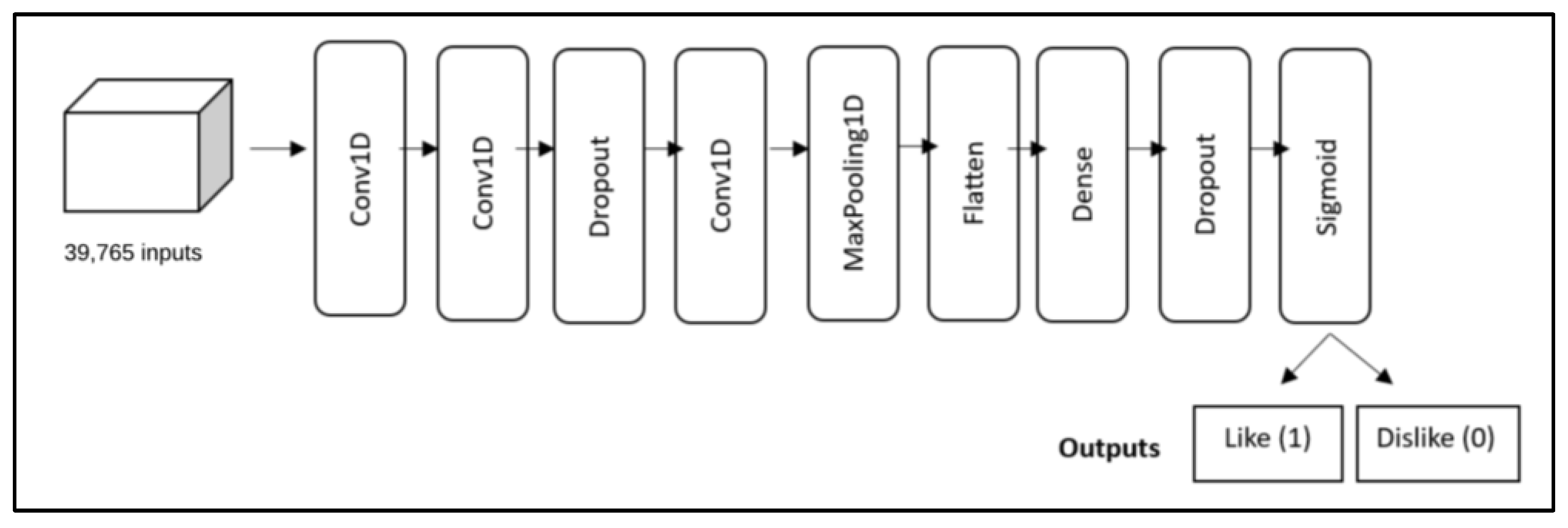
The CNN architecture employed in this work is shown in
Figure 4. The CNN model consists of two convolutional (conv1d) blocks, both with 32 filters. Then, a 0.3 dropout regularization is used to improve the performance of the model via a modest regularization effect, followed by a third conv1d layer with 64 filters. The kernel size of all conv1d filters is 3 × 3, with zero padding and stride, and we used the Rectified Linear Units (Relu) as the activation function due to its unity gradient, where the maximum amount of error is passed during backpropagation.
Next, a maximum subsampling layer (max pooling layer) of a 2 × 2 subwindow was applied, followed by a flattening layer. Then, a fully connected dense layer with 128 units was applied to have nonlinearity properties, followed by a 0.3 dropout regularization. The network ends with a connected dense layer fed with a sigmoid activation function for binary classification.
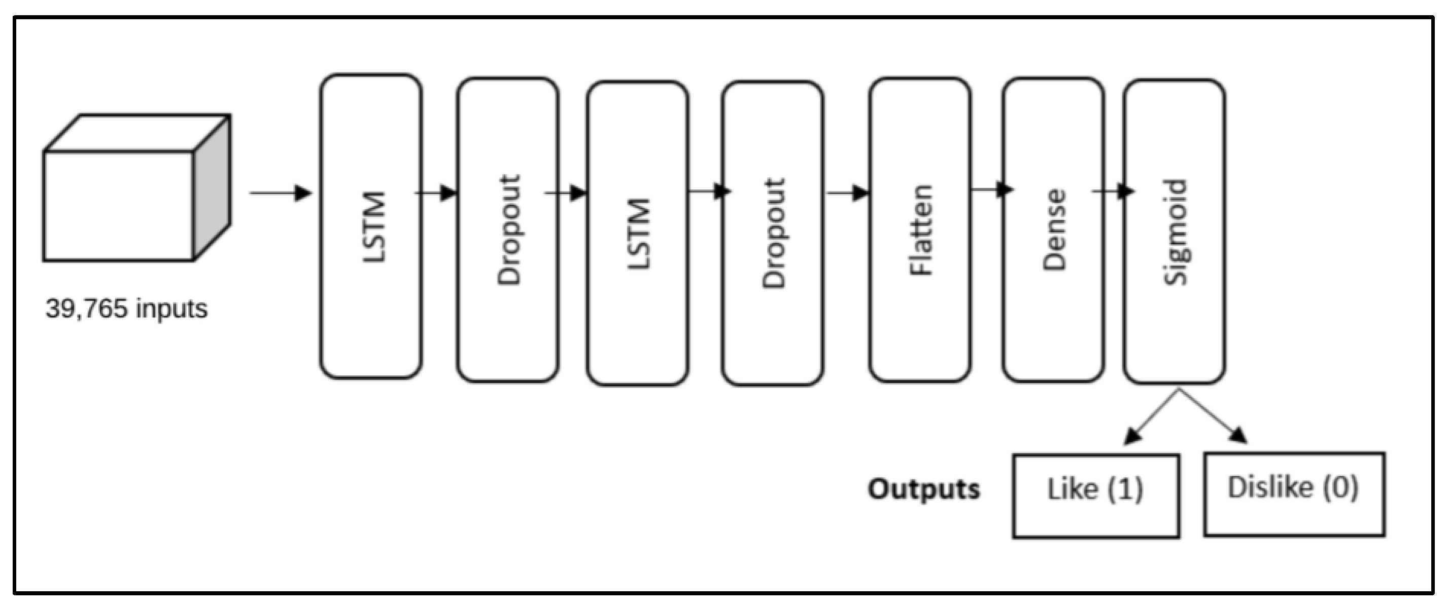
5.5.2. LSTM Architecture
We used the standard formulation of LSTMs with the logistic function (σ) on the gates and the hyperbolic tangent on the activations. The model has two LSTM layers with dropouts in between, followed by a flattening layer. Then, the output is passed to the fully connected network. The Relu activation function is used to predict the final output. The block diagram of the LSTM architecture is shown in
Figure 5.
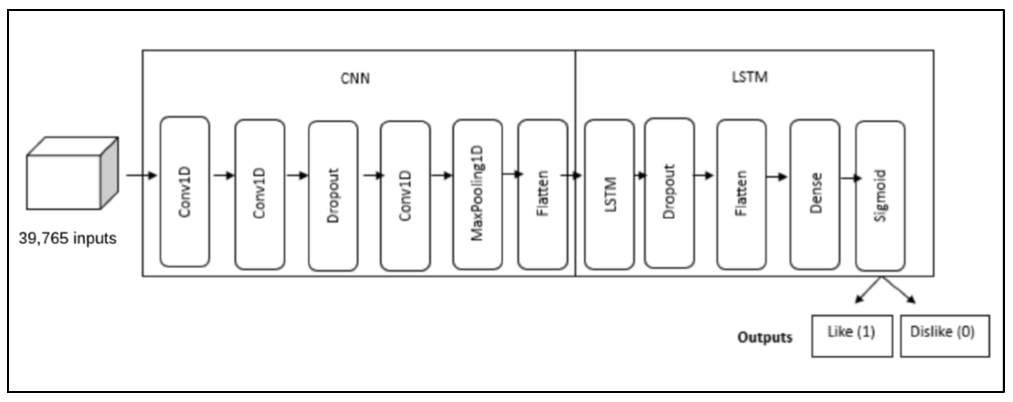
5.5.3. Hybrid Architecture
To build our hybrid architecture, we performed design experiments in various ways. For example, we tested whether to best start the hybrid cascade model with the CNN followed by the LSTM or vice versa. We also tested a different number of layers and filters. The final hybrid architecture used is illustrated in
Figure 6.
This architecture starts with the CNN model consisting of two conv1d blocks, both with 128 filters. Then, a 0.3 dropout regularization is used to improve the performance of the model via a modest regularization effect, followed by a third conv1d layer with 128 filters.
The kernel size of all conv1d filters is 3 × 3 with zero padding and stride, and the activation function employed is the hyperbolic tangent function (Tanh) because it is a differentiable function with smooth and continuous derivatives. This helps propagate gradients through the network during the backpropagation process, which makes training more stable. Then, a maximum subsampling layer (max pooling layer) of a 2 × 2 subwindow was applied, followed by a flatten layer.
Next, this architecture is passed through the LSTM model with the logistic function on the gates and the hyperbolic tangent on the activations. The model has one LSTM layer with a 0.25 dropout, followed by a flattening layer. The output is then passed to the fully connected network with the Relu activation function and 32 filters. The network ends with a connected dense layer fed with the sigmoid activation function for binary classification.
6. Results and Discussion
For model evaluation, we discuss the results of the proposed models themselves and compare their performance with existing methods and previous studies that used SEED.
First, we assessed the predictive performance of our proposed models (CNN, LSTM, and the hybrid model) using commonly used ML metrics: accuracy, precision, and recall (
Table 2). We also used the confusion matrix and the learning curves of accuracy, training loss of 80%, and validation loss of 20% over epochs.
Accuracy is the percentage of the total number of correct predictions that actually occurred. Precision is the percentage of properly identified positive cases. Recall is the percentage of real positive cases that were properly identified [
40].
We achieved the highest performance in classification choice through our proposed LSTM model after resampling the dataset with 96% accuracy and 95% for both precision and recall. The hybrid model came in second with 91% accuracy, followed by CNN with 88% accuracy.
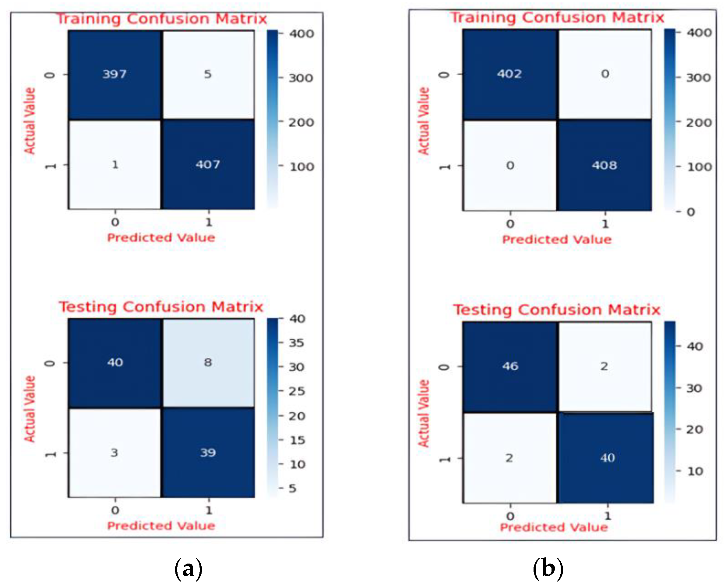
In our study, we considered all three evaluation measures because the ML model needs to truly identify and not miss the like states as positive emotions and not misclassify the actual dislike states as like states. The confusion matrix is used to understand what type of mistakes (like or dislike) our proposed models made during the training and testing phases.
Figure 7 shows the number of actual choice states versus the predicted choice states for our proposed models, CNN and LSTM.
The error rate (misclassification rate) of the LSTM model was 0.4. It predicted two wrong like states (false positive) and two wrong dislike states (false negative). In contrast, the error rate of the CNN model increased to 0.11. It predicted eight false like states (false positive) and three false dislike states (false negative).
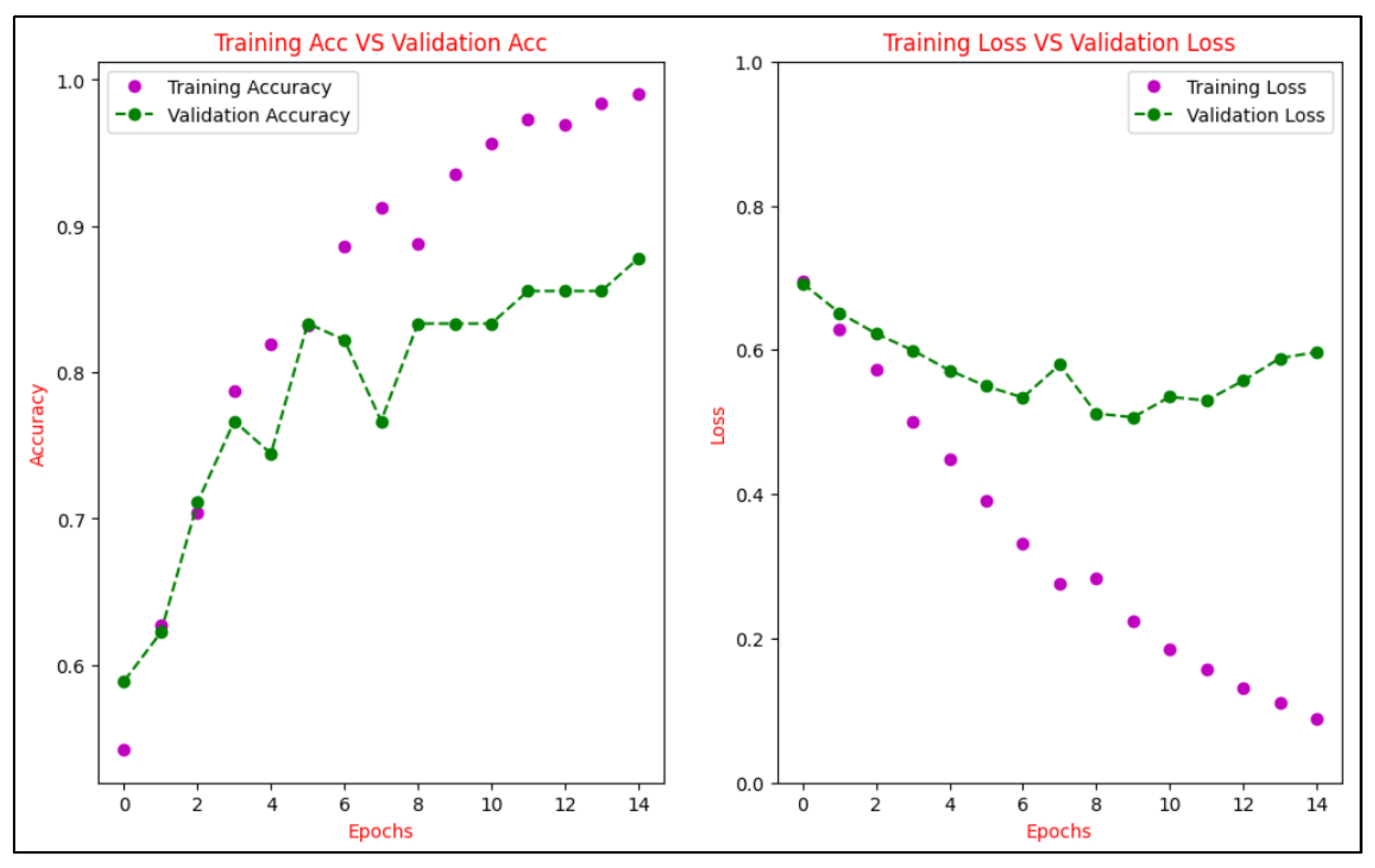
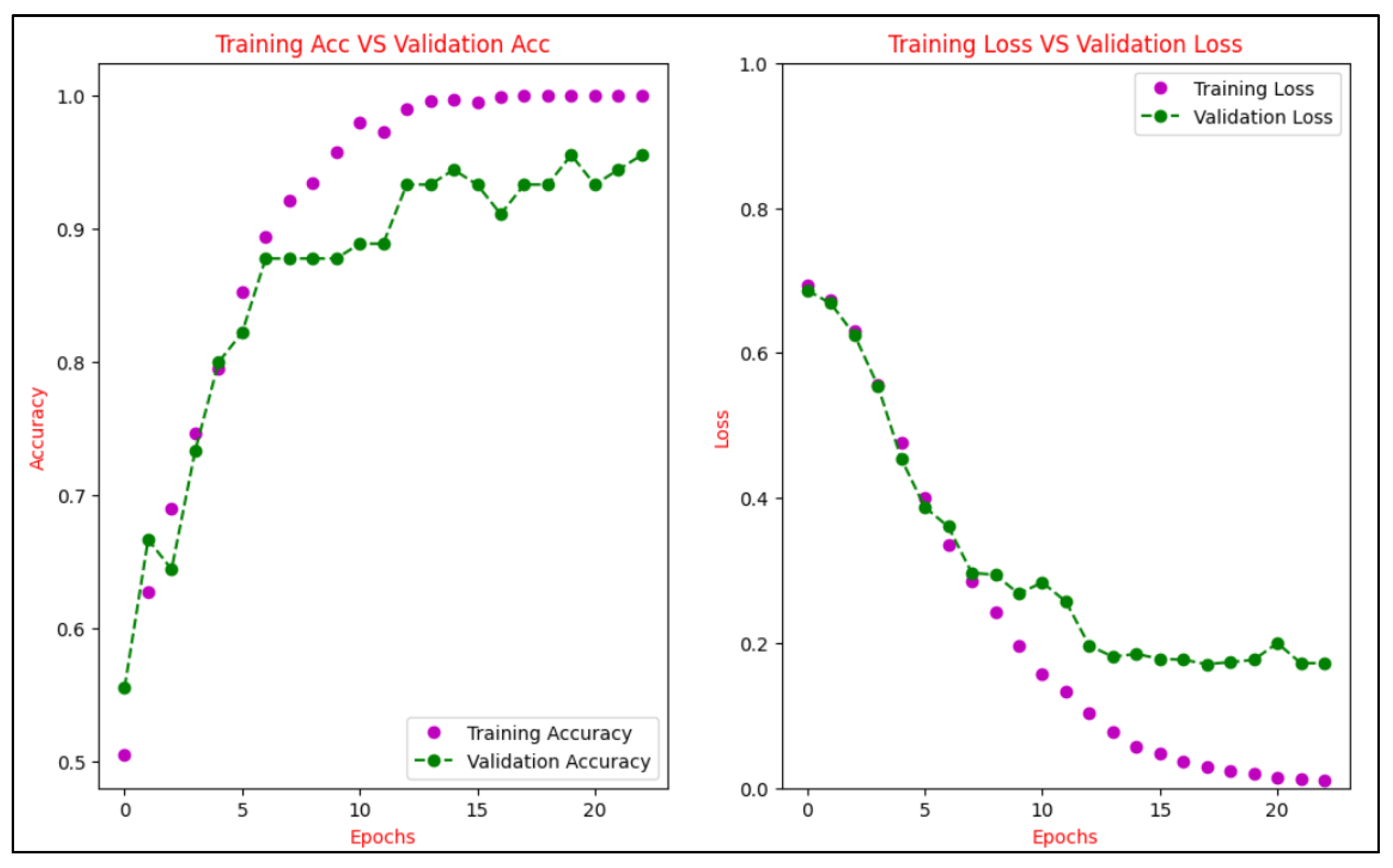
To ensure that our proposed model has no over- or under-fitting problems, learning curves are used to display the change in training accuracy versus validation accuracy over epochs and the training loss versus validation loss over epochs.
Figure 8 depicts the CNN model’s accuracy and loss during the training and validation phases. As shown in the plots, the model converged slowly over epochs, and the convergence stopped after epoch 10.
Figure 9 depicts the LSTM model’s accuracy and loss during the training and validation phases. As can be observed from the graph, the model converged over epochs faster than the CNN model, and it is normally fitted with the highest accuracy and the least loss.
6.1. Comparison with Classical Classifiers
We used different existing classic ML classifiers such as KNN, SVM, RF, LG, AdaBoost, and XGBoost to compare their performance with the proposed DL models. Our extracted features are fed into these classifiers, and we investigated several parameters for each one. We evaluated the performance of each classifier in the same dataset twice (before and after resampling) using the three evaluation metrics: accuracy, precision, and recall.
Table 3 shows the hyperparameters used in the classical classifiers as follows:
For KNN, we used 10 for the number of neighbors using all processors.
For SVM, we used the polynomial kernel function and a cost of 10.
For LR, we used the liblinear solver with a 100 regularization strength.
For RF, we built 500 decision trees during the training and produced the class that represents the mode of the choice.
For XGBoost, we used binary logistics.
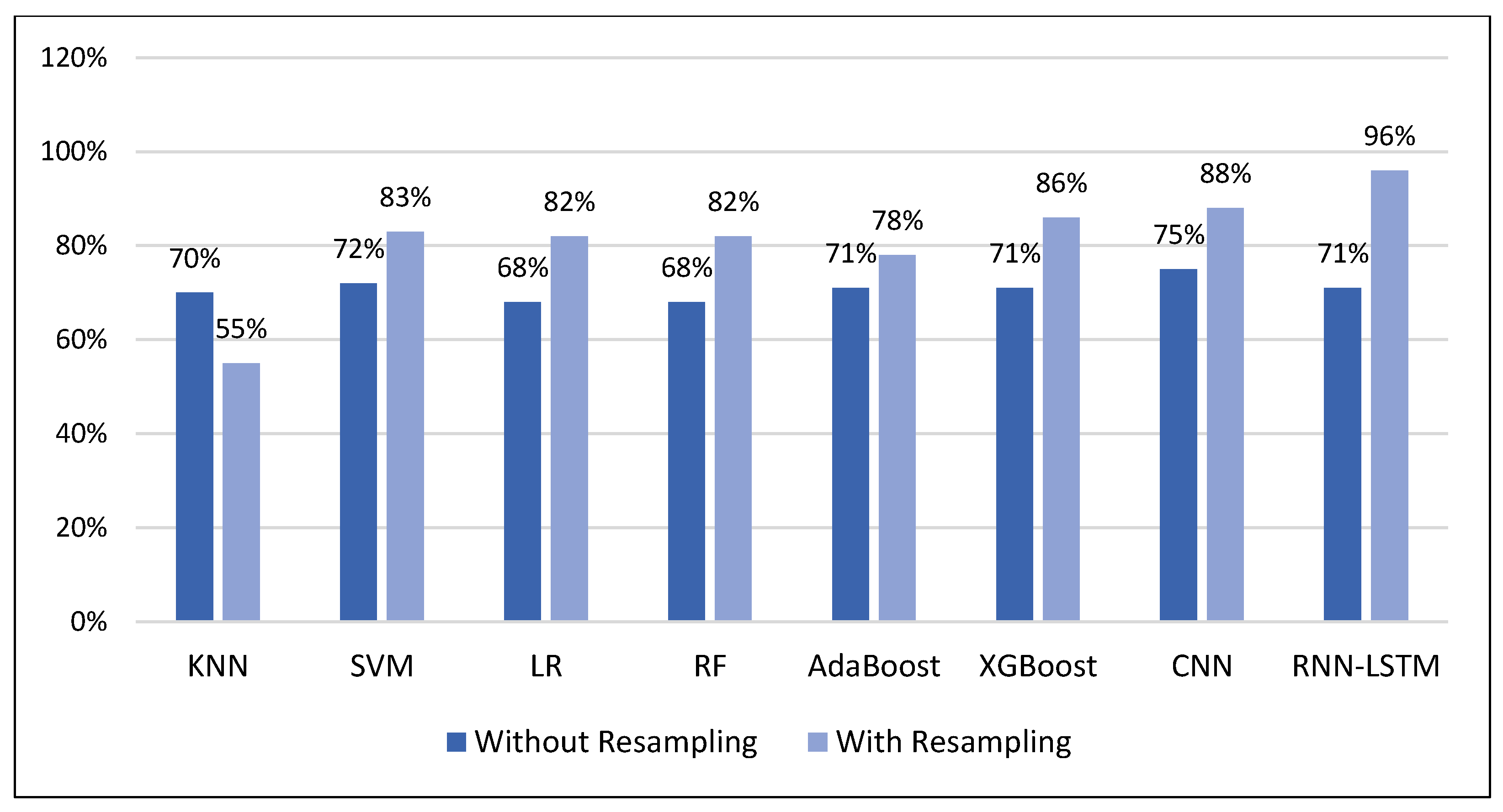
Figure 10 shows that for the dataset before resampling, the performance of all classifiers was similar in terms of accuracy (about 70%). However, for the dataset after resampling, the performance of all classifiers, except for KNN, increased significantly. The KNN performance decreased after resampling to about 55% because of the enlarged number of samples, and KNN performs better with the smallest datasets. The highest performance was reached with LSTM (96%), followed by CNN (88%), XGBoost (86%), SVM (83%), LR and RF (82%), and AdaBoost (78%).
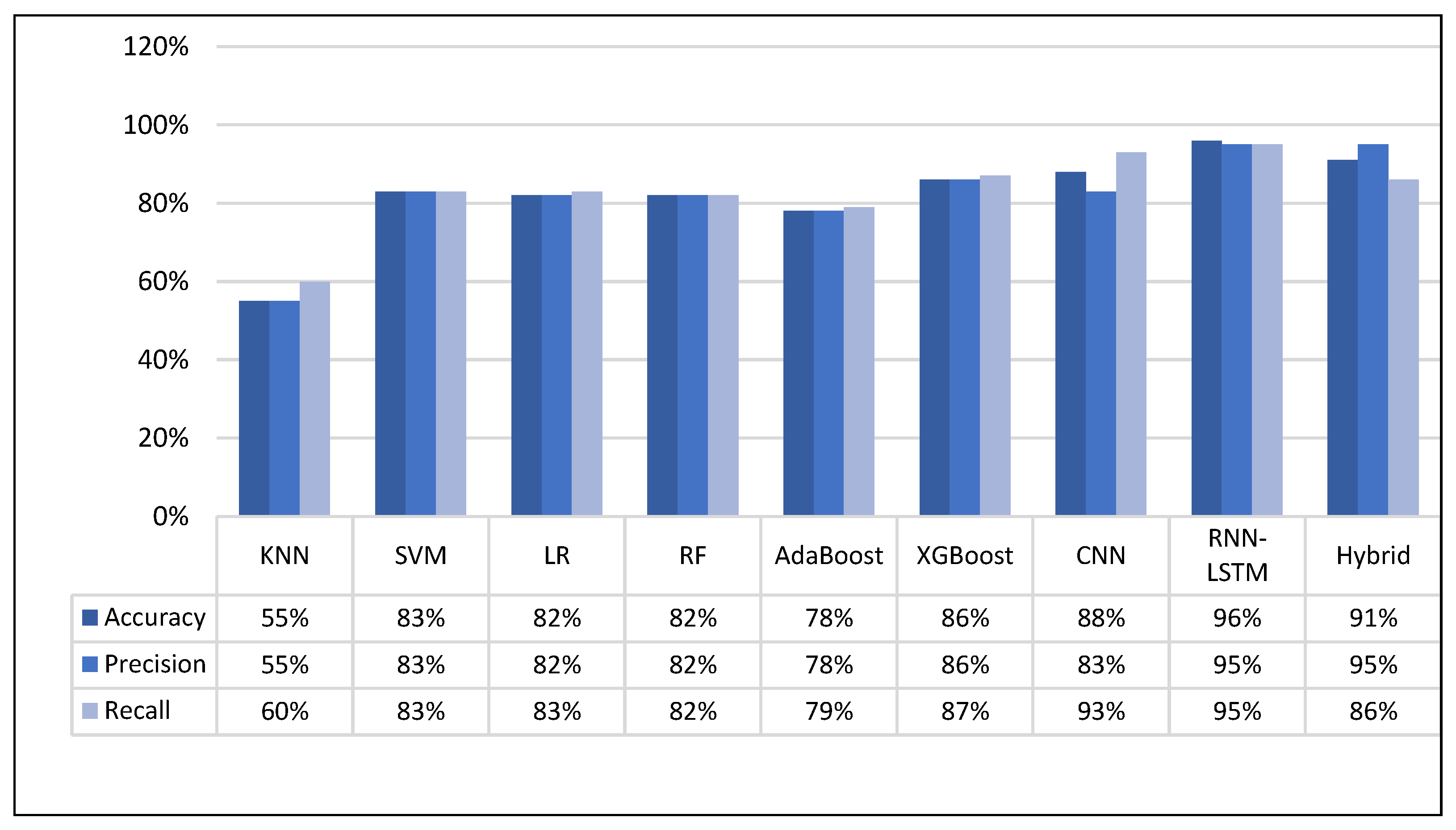
Figure 11 shows the comparison of the performance measurements (accuracy, precision, and recall) of the models after resampling. The proposed LSTM achieved the best accuracy at 96% over the hybrid model (91%), whereas the KNN achieved the lowest at 55%. AdaBoost achieved a higher accuracy of 78% compared with KNN. The performance of the three classifiers, SVM, LR, and RF, was very similar at 83%, 82%, and 82%, respectively. Of all classical classifiers, XGBoost had the best performance (86%), which is close to that of our proposed CNN (88%).
6.2. Comparison with Previous Studies
We assessed our proposed models and compared their results with those of previous studies that used SEED with different extracted features and various classification methods. The comparison in
Table 4 shows that our LSTM model provided promising results.
In this paper, we achieved similar results to [
18], with the hybrid model and CNN reaching accuracies of 93.46% and 89.53%, respectively. Our work also achieves similar results to [
29], which achieved 90.12% accuracy using RNN with LSTM for eight channels. Further, the accuracies reached by our SVM and LR are 83% and 82%, respectively, corresponding to researchers’ work [
8] for SVM and LR, which were 83.99% and 82.70%, respectively.
Based the feature extraction techniques, we notice that LSTM performs better with PSD and DE at 96% compared to WT that achieved 90.12% [
29]. The reasons behind the improved accuracy, including the ability of spectral features to capture frequency-specific information and the complementary nature of statistical features.
To summarize, in the SEED dataset, the emotional stimuli were task-relevant, as participants were required to recognize an image, which likely contributed to the manifestation of the emotional response in the EEG signals. Instead of 62 channels, we used 12 channels to extract features that were fed to our models. This reduces computation time and can be more useful for EEG datasets recorded using devices with fewer channels. Unlike other research, we combined multiple extracted features to indicate choice states, such as choice indices and DE. We achieved good results with our proposed LSTM model, with 96% accuracy. Compared with previous studies that used SEED, our work used the least number of electrodes and more different feature sets and classifiers.
7. Conclusions
Neuroscientists use EEG-based BCI to measure brain activity and find the neural correlates of decision-making processes, which involve both cognitive and emotional factors. By employing AI and DL, it becomes feasible to make more accurate predictions regarding the outcomes of decisions and individuals’ behavior and choices [
28].
This research has demonstrated the potential of utilizing DL models and EEG signals to build an accurate individual choice prediction system. The proposed LSTM model achieved a high accuracy rate of 96%, which outperformed classical classifiers and the results of previous studies that used SEED.
The use of fewer channels for feature extraction reduced computation time and increased the practicality of the model for EEG datasets recorded using devices with fewer channels. Overall, this study provides valuable insights into the development of accurate prediction models for individual choices and behavior using EEG signals.
For future work, we plan to investigate the role of feature selection of the extracted features to improve the performance of detecting the choice states in the SEED dataset.


