Real Image Deblurring Based on Implicit Degradation Representations and Reblur Estimation

Abstract

Most existing image deblurring methods are based on the estimation of blur kernels and end-to-end learning of the mapping relationship between blurred and sharp images. However, since different real-world blurred images typically have completely different blurring patterns, the performance of these methods in real image deblurring tasks is limited without explicitly modeling blurring as degradation representations. In this paper, we propose ${\mathrm{IDR}}^2\mathrm{ENet}$, which is the Implicit Degradation Representations and Reblur Estimation Network, for real image deblurring. ${\mathrm{IDR}}^2\mathrm{ENet}$ consists of a degradation estimation process, a reblurring process, and a deblurring process. The degradation estimation process takes the real blurred image as input and outputs the implicit degradation representations estimated on it, which are used as the inputs of both reblurring and deblurring processes to better estimate the features of the blurred image. The experimental results show that whether compared with traditional or deep-learning-based deblurring algorithms, ${\mathrm{IDR}}^2\mathrm{ENet}$ achieves stable and efficient deblurring results on real blurred images.

1. Introduction

Image deblurring is a classical topic in the field of low-level computer vision, with the aim of converting blurred images into corresponding sharp images and thus recovering the information contained in them. There are various factors involved in image blurring, such as camera shake, lack of focus, fast motion of the target object, etc. [1]. Blurred images can be expressed as follows:

$$y=\mathcal{M}(x;\theta )$$

(1)

where x is the real sharp image corresponding to the blurred image y, $\mathcal{M}(·)$ is the image blur function, and $\theta$ is the parameter vector of $\mathcal{M}(·)$. The goal of image deblurring is to recover the sharp image, i.e., to find the inverse of the image blur function in (1), as follows:

$$x_{de}={\mathcal{M}}^{-1}(y;\theta )$$

(2)

where ${\mathcal{M}}^{-1}(·)$ is the deblur function, and $x_{de}$ is the deblurred image, which is the estimation of potential sharp image x.

Early deblurring research modeled the blurring process as a convolution of the blur kernel with the image, at which point Equation (1) degenerated to

$$y=K\ast x+n$$

(3)

where K denotes the blur kernel, n denotes the additional Gaussian noise and ∗ denotes the convolution operator. Then, the deblurring task transformed into an inverse-filtering problem, focusing on how to find and estimate the blur kernel [2,3,4,5,6,7]. However, in real scenes, the blurring of different images may be formed by completely diverse degradation patterns, which leads to the estimation of a single blurring kernel that cannot be well applied to real-world image deblurring. To address this problem, scholars have proposed a series of end-to-end methods for learning the mapping relationship between blurred and sharp images [8,9,10], which are mostly based on deep learning networks, such as Convolutional Neural Networks (CNN) [11,12,13,14,15] and Generative Adversarial Networks (GAN) [10,16,17,18]. Among CNN-based works, better results have been achieved in recent years based on Deep Auto-Encoders (DAE), which fuse U-Net network structures [17,19,20]. Shen et al. [20] set up an a priori face parsing/segmentation network to predict face labels before U-Net, and then the blurred images were fed into U-Net along with the predicted face labels to obtain the deblurred images. Other approaches analyze multiple DAEs and U-Nets in an attempt to construct cascade networks, where one U-Net produces a coarse deblurred image and then feeds into the second U-Net to obtain better deblurring performance. Among the GAN-based approaches, Nah et al. [8] were the first to introduce the adversarial loss function ${\mathcal{L}}_{adv}$. They then constructed an eleven-layer discriminator, which is trained with real sharp images as the input and computes ${\mathcal{L}}_{adv}$ based on whether it can eventually distinguish deblurred images from real sharp images. Subsequent GAN-based approaches basically follow this idea [10,16,21]: the generator G generates a deblurred image $x_{de}$, and the training is considered to be finished if G fools the discriminator D so that it cannot distinguish between the generated image $x_{de}$ and the real sharp image x. Kupyn et al. [10,16] proposed DeblurGAN, whose generator consists of two-stride layers of convolution blocks, nine layers of residual blocks and two transposed convolution blocks. The DeblurGANv2 proposed on this basis introduces the results of relativistic conditional GAN [22], whose generator uses a pyramidal-feature architecture, while its discriminator uses the Double-Scale RaGAN-LS Discriminator, thus improving the efficiency and performance of the whole network. However, whether U-Net or GAN, the end-to-end-based learning methods mentioned above lack the exploitation of image degradation representations such that their performance in real-world deblurring tasks is still limited. In addition, blurred regions in blurred images usually show greater variation than noisy points or high-frequency texture details, so the learning and estimation of the degradation process is important for better reconstruction.

Based on the above issues, and inspired by the work of Dong et al. [23], Zhai et al. [24], Qin et al. [25] and Li et al. [26] on image restoration, we propose a real image deblurring network based on the implicit degradation representations and reblur estimation with an encoder–decoder structure, called ${\mathrm{IDR}}^2\mathrm{ENet}$. More specifically, the network framework contains three main processes, degradation estimation, reblurring, and deblurring, which consist of a degradation estimation subnetwork, a multi-scale degradation-representation-guided deblurring subnetwork and a multi-scale degradation-representation-guided reblurring subnetwork, respectively. The main contributions of this paper can be summarized as follows:

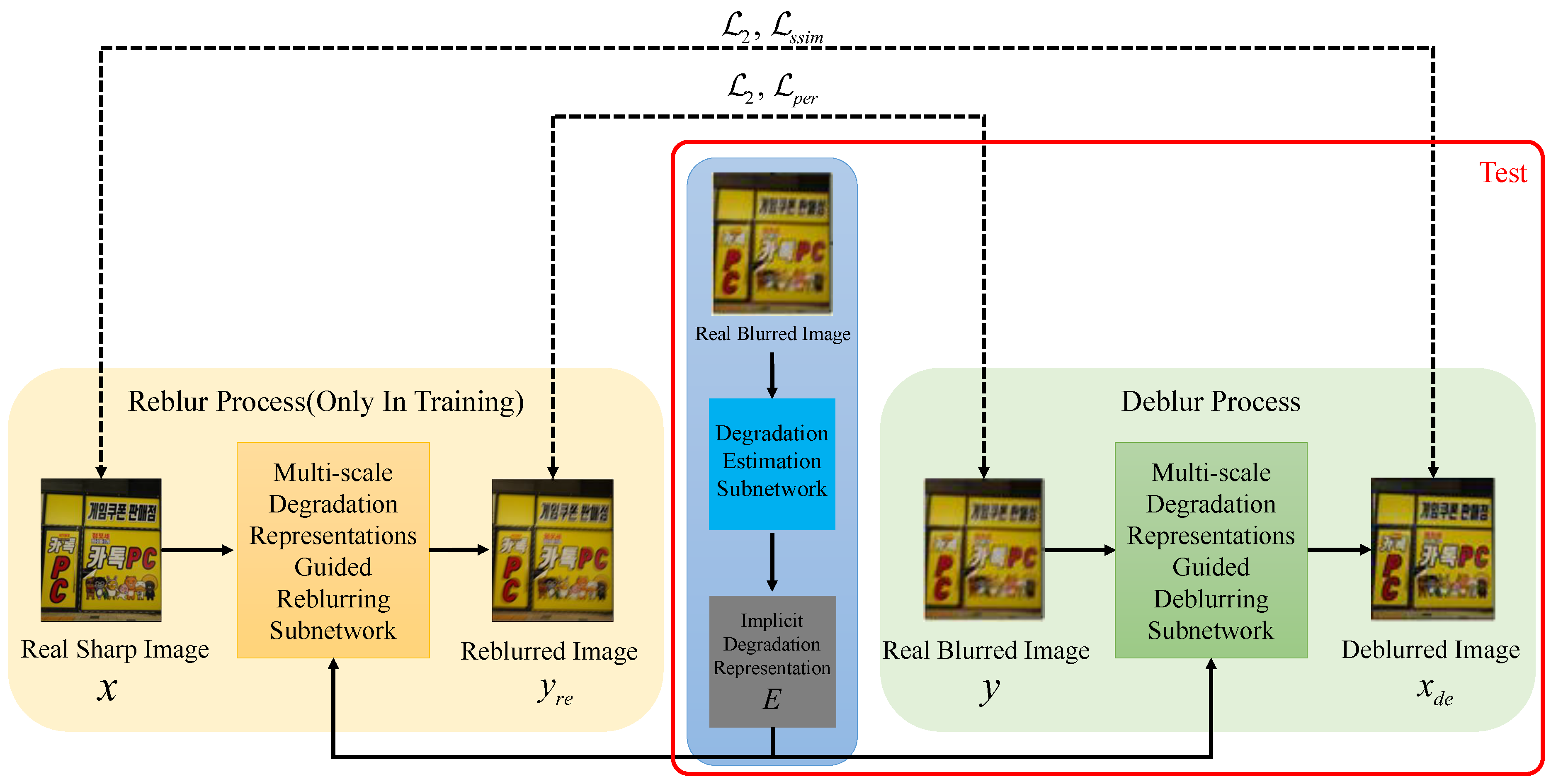
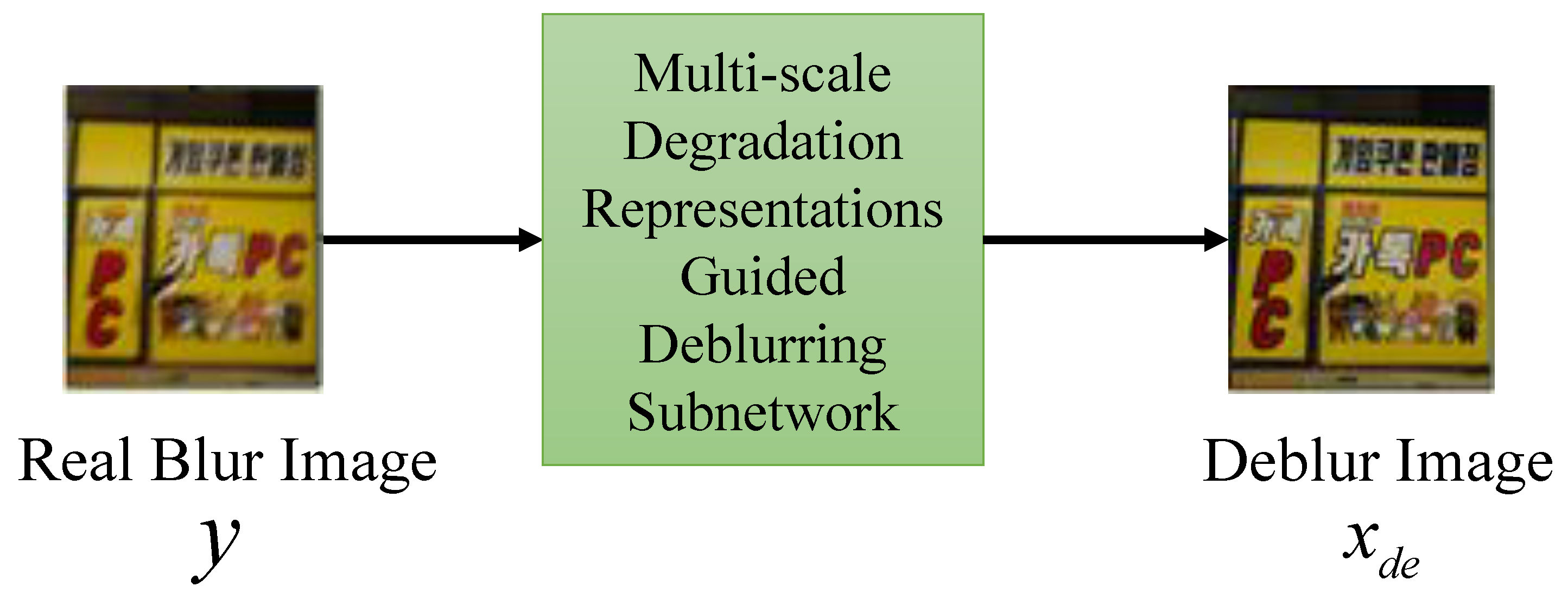
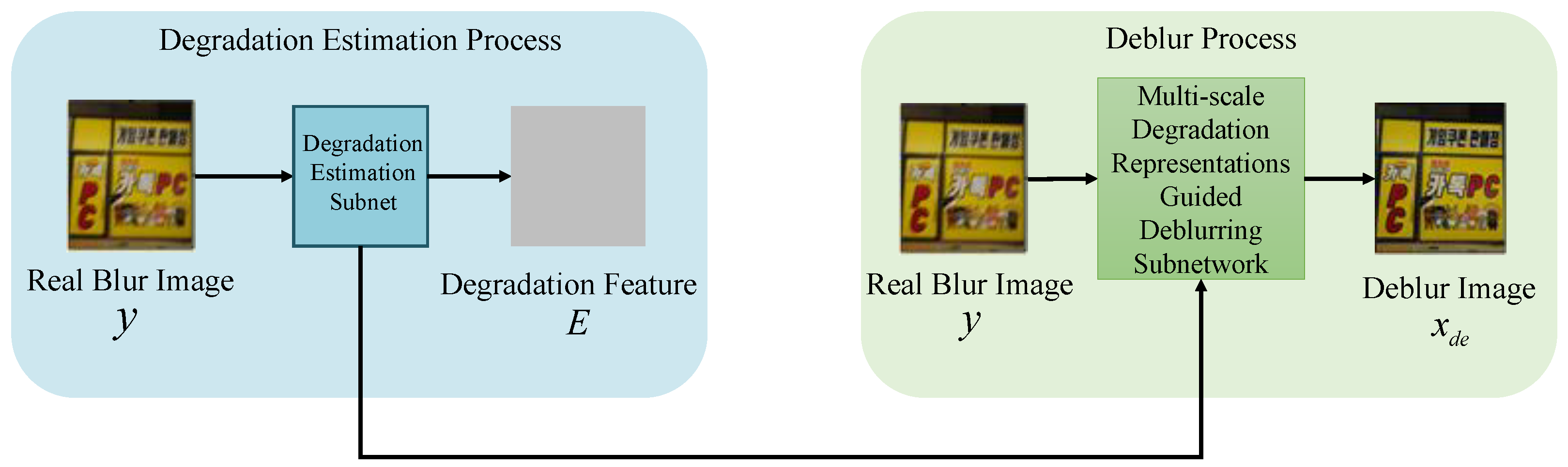
• We propose an implicit degradation representation and reblur estimation network called ${\mathrm{IDR}}^2\mathrm{ENet}$. The network learns and estimates implicit degradation representations in real images by reblurring sharp images (generating a reblurred image from a real sharp image that resembles a real blurred image). The degradation representations are then used to guide the deblurring process for better reconstruction. Estimating and using the degradation representations in this way has two advantages: (1) there is no need to model the complex degradation process in the real blurred image; and (2) the degradation representations estimated in a learning way can be adapted to the blurring in different images.
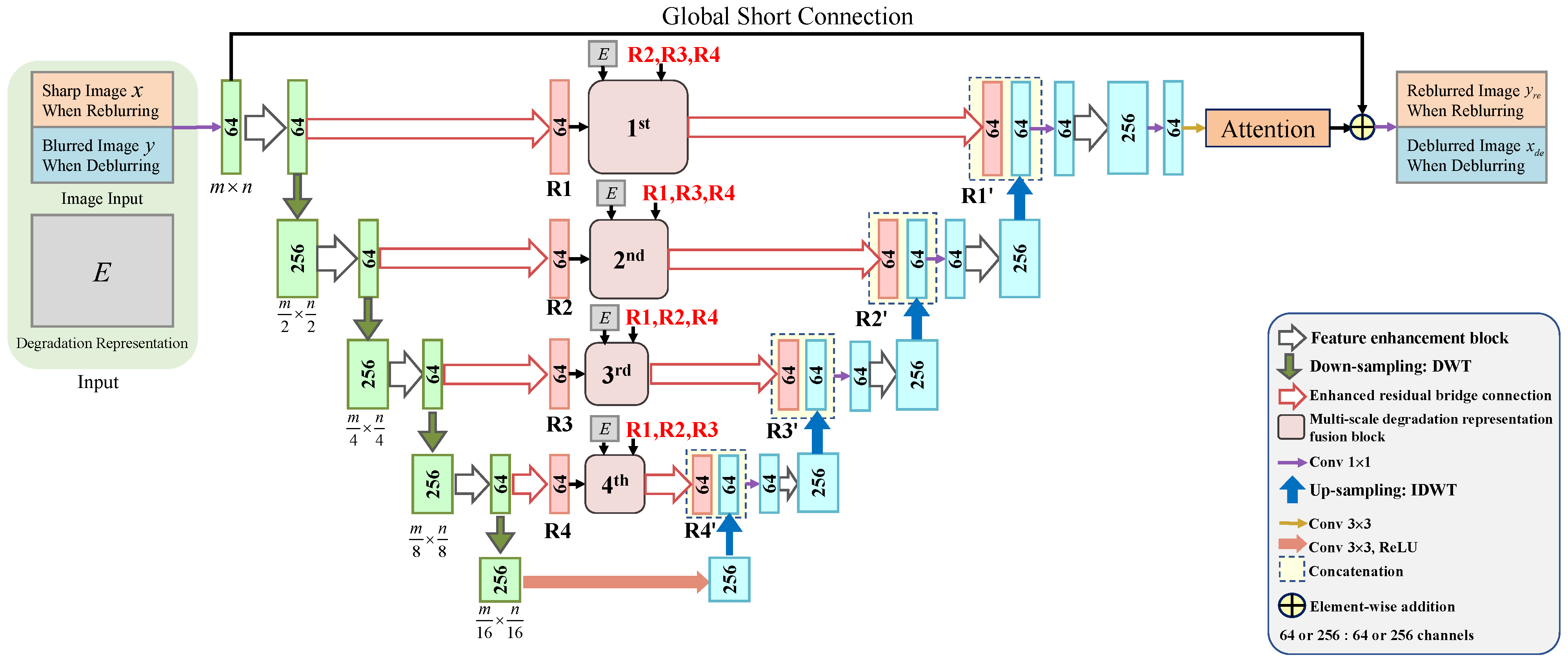
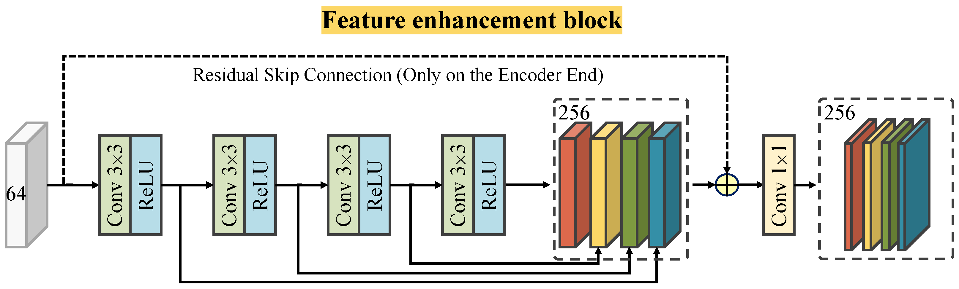
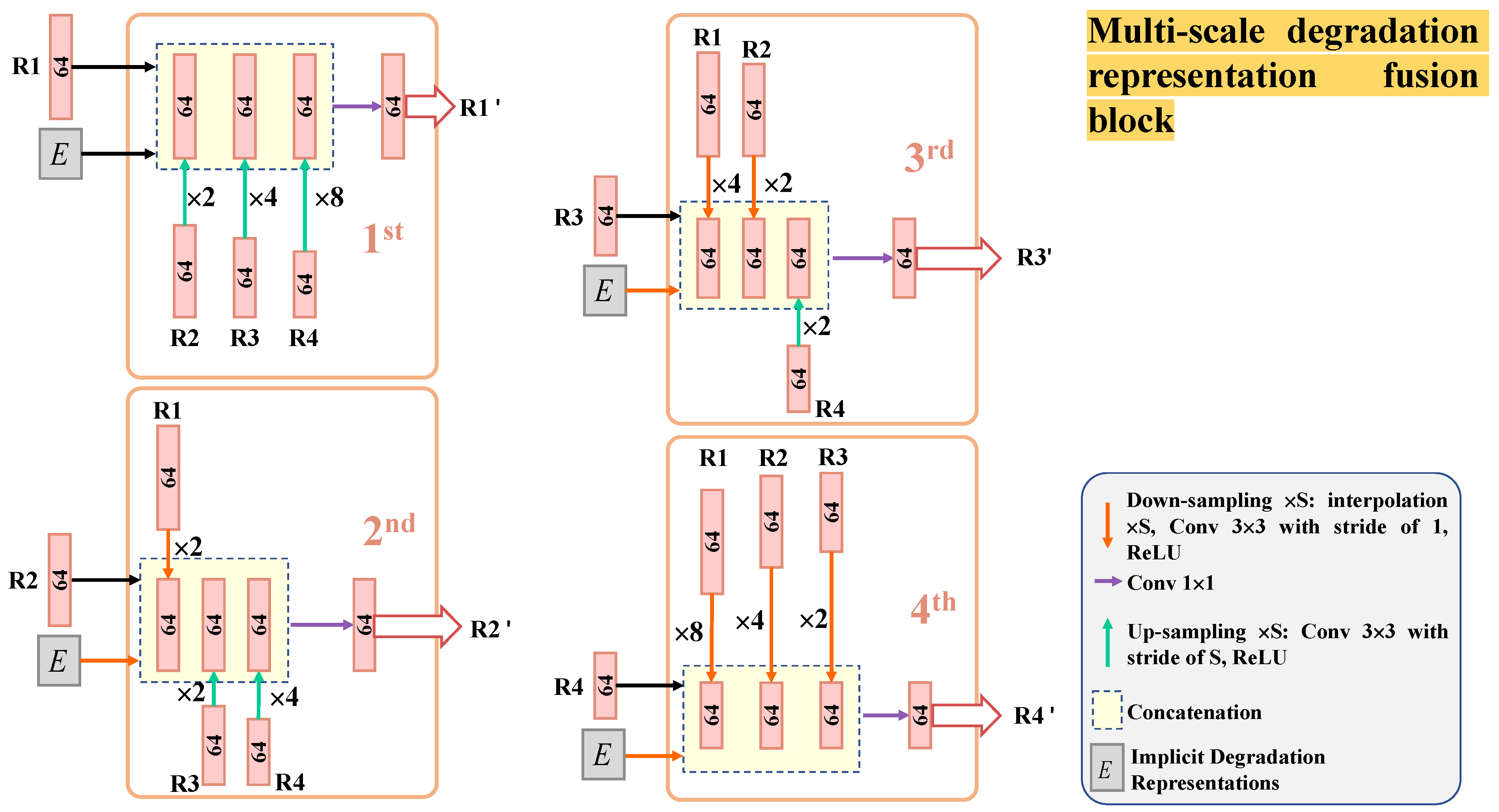
• In terms of network structure, in order to fully utilize the degradation representations, we designed a multi-scale degradation representation fusion module, which is integrated into the reblurring subnetwork and deblurring subnetwork, and is used both for training and testing. We also conduct an ablation study to demonstrate the effectiveness of implicit representation estimation. Our results show that our network achieves stable and efficient outcomes on multiple datasets.

2. Related Work

2.1. Blind Image Deblurring

Image deblurring can be divided into two categories: non-blind deblurring (a priori known blur kernel K) and blind deblurring (unknown K). Since the degradation representations of real-world blurred images are spatio-temporal variants [4,27,28], non-blind deblurring methods cannot accommodate blur changes due to object movement and scene depth. Therefore, blind deblurring is now more widely studied. Although the blur kernel is unknown, early blind deblurring works still assume that it is uniformly distributed throughout the whole image [2,29]. However, real-world blurred images often have different blurring regions of an image composed of various blur kernels. Methods based on the a priori assumption of uniform blur kernels do not perform well in dynamic scenes due to camera shake and 3D blurring. To solve this problem, scholars have proposed many deep-learning-based methods for dynamic scene deblurring [8,9,19]. Nah et al. [8] present a multi-scale CNN-based network to directly map the various source-blurred images to latent sharp images. Tao et al. [9] proposed a scale-recurrent network(SRN-DeblurNet), whose input is a series of multi-scale blurred images. SRN-DeblurNet then learns blurring features in the images and outputs the corresponding sharp images through the encoder–decoder structure of residual blocks, residual skip connections, etc. The network proposed by Gao et al. [19] also adopts an encoder–decoder structure to extract the blurred features. Unlike Tao et al. [9], they added Parameter Selective Sharing for CNN parameters to the network in order to achieve better deblurring performance. However, the methods mentioned above do not sufficiently extract the degradation representations of blurred images, which leads to a decrease in deblurring performance in the face of more complex real blurred images.

2.2. Reblur to Deblur and Degradation Estimation

Aside from deep auto-encoders (DAE), generative adversarial networks (GAN) and multi-scale networks, reblurring networks have been widely studied in recent years due to their ability to generate additional blurred images for learning [30,31,32]. Zhang et al. [31] propose a novel network combining two GAN-based models, learning-to-Blur GAN (BGAN) and learning-to-DeBlur GAN (DBGAN). The BGAN learns to convert a sharp image to a reblurred image, and DBGAN learns to recover the latent image from BGAN. Such multi-GAN structures are very innovative, but due to the inherent limitations of GAN-based networks, their performance on traditional deblurring metrics such as PSNR and SSIM is not very good. Moreover, the final deblurring performance of the network proposed by Zhang et al. [31] depends more on the generative adversarial structure, i.e., whether the discriminator D of DBGAN can distinguish between (real) sharp and deblurred (fake sharp) images, and does not explicitly extract the blurring features of blurred images themselves.

Some recent deblurring works treat image blurring as a kind of degradation and achieve deblurring by extracting the degradation representations of the blurred images [24,25,26,33]. Zhai et al. [24] proposed a novel CNN-based iterative network, and incorporated a gradient descent algorithm in the design of the deep network, resulting in state-of-the-art results. Qin et al. [25] instead designed multiple modules to extract and utilize degradation representations in a multi-scale manner, including residual blocks, a feature fusion module, skip connections, and attention, so that the obtained degradation representations can reflect the nature of the blurred image itself more comprehensively.

Inspired by the above works [24,25,26,33], we propose a deblurring method based on implicit degradation representations and reblur estimation. It can effectively combine the advantages of the above-mentioned reblurring estimation and degradation extraction, which not only effectively extracts and utilizes the degradation representations of the blurred image itself, but also allows the network to learn the degradation representations better through the reblurring process, thus making the deblurring results more stable and improving their quality.

3. Proposed Method

3.1. Network Structure

As shown in Figure 1, ${\mathrm{IDR}}^2\mathrm{ENet}$ contains a degradation representation estimation process, a reblurring process and a deblurring process during training, whose architecture is mainly inspired by [24,25,26,33]. The degradation representation estimation process is dominated by the degradation estimation subnetwork, whose input is a real blurred image y, and whose output is implicit degradation representations E estimated by learning on y.

The deblurring process takes the real blurred image y and the degradation representation E as input, and outputs a sharp image $x_{de}$ after deblurring. E enables the multi-scale degradation-representation-guided deblurring subnetwork to learn the corresponding blur features in blurred images, so that it can adaptively handle a wide range of blurred images. It is worth mentioning that the multi-scale degradation-guided deblurring subnetwork does not learn a complete mapping from the real blurred image y to the deblurred image $x_{de}$; instead, it only learns the residuals between them, which can be expressed by the following equation:

$$x_{de}={\mathcal{N}}_{\mathrm{Deb}}(y,E)$$

(4)

where ${\mathcal{N}}_{\mathrm{Deb}}$ denotes the multi-scale degradation-guided deblurring subnetwork.

In order to better learn degradation representations, the design uses the reblurring process. An immediate idea is that the reblurring subnetwork learns to generate the reblurred image $y_{re}$ using only the sharp image x as input. However, since a sharp image can correspond to countless blurred images, in order to reduce training difficulty and assist the degradation estimation subnetwork to better estimate the degradation representations, the real sharp image x and degradation representation E are used together as the input of the reblurring subnetwork, which is also expressed as a multi-scale degradation-representation-guided reblurring subnetwork, with y as the target and the output as the reblurred image $y_{re}$. Likewise, the multi-scale degradation-guided reblurring subnetwork learns only residuals between the sharp image x and reblurred image $y_{re}$ to better implement degradation representation E to guide reconstruction. The equation of the deblurring process is expressed as follows:

$$y_{re}={\mathcal{N}}_{\mathrm{Reb}}(x,E)$$

(5)

where ${\mathcal{N}}_{\mathrm{Reb}}$ represents the multi-scale degradation-guided reblurring subnetwork. This is intended to, on the one hand, guide the degradation estimation subnetwork to focus more on learning in order to extract the degradation representation E in the image during the reblurring process and ignore the content of the image itself, and on the other hand, to make the training process faster and more stable.

During training, the degradation estimation subnetwork, multi-scale degradation-guided reblurring and deblurring subnetwork are trained jointly. This has the advantage of constraining the degradation estimation subnetwork to better estimate E in the joint training on the one hand, and enable the multi-scale degradation-guided deblurring subnetwork to better utilize degradation representations for reconstruction on the other. For testing, ${\mathrm{IDR}}^2\mathrm{ENet}$ only retains the degradation estimation and deblurring process.

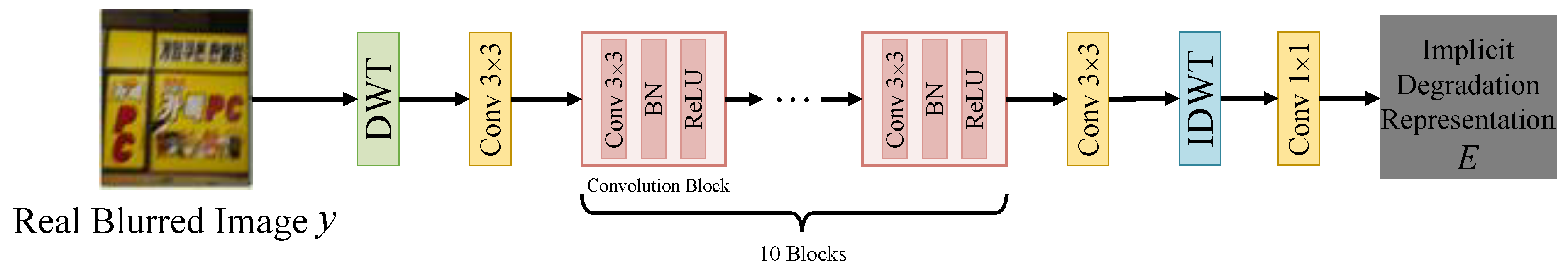
3.2. Degradation Estimation Subnetwork

As shown in Figure 2, the degradation estimation subnetwork takes the real blurred image y as the input and outputs the estimated degradation representation E, whose structure is inspired by the work of Qin et al. [25]. In order to encourage the subnetwork to better learn and estimate degradation representation, discrete wavelet transform (DWT) pairs are designed at the beginning and end of the subnetwork. y is converted to a smaller size with an increasing dimensionality through DWT, followed by initial feature extraction through a $3\times 3$ convolutional layer and learning in a cascade of 10 convolutional blocks. Then, symmetrically with input, the image is passed through one $3\times 3$ convolution layer and one inverse discrete wavelet transform (IDWT) layer in order to achieve size recovery. Finally, a $1\times 1$ convolution layer is used to transform the output after IDWT into 64 channels of high dimensionality. Compared with the single explicit blur kernel estimated in the general method, implicit degradation representations of 64 channels can better adapt to the complex spatially variant degradation representations in real blurred images and possesses a stronger expression of them.

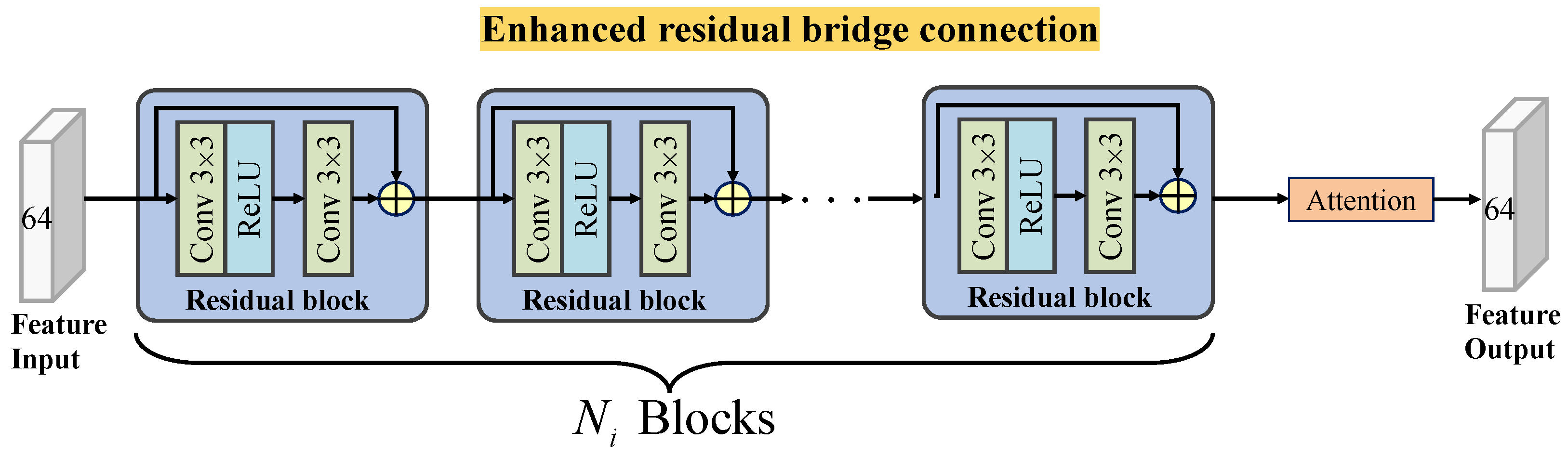
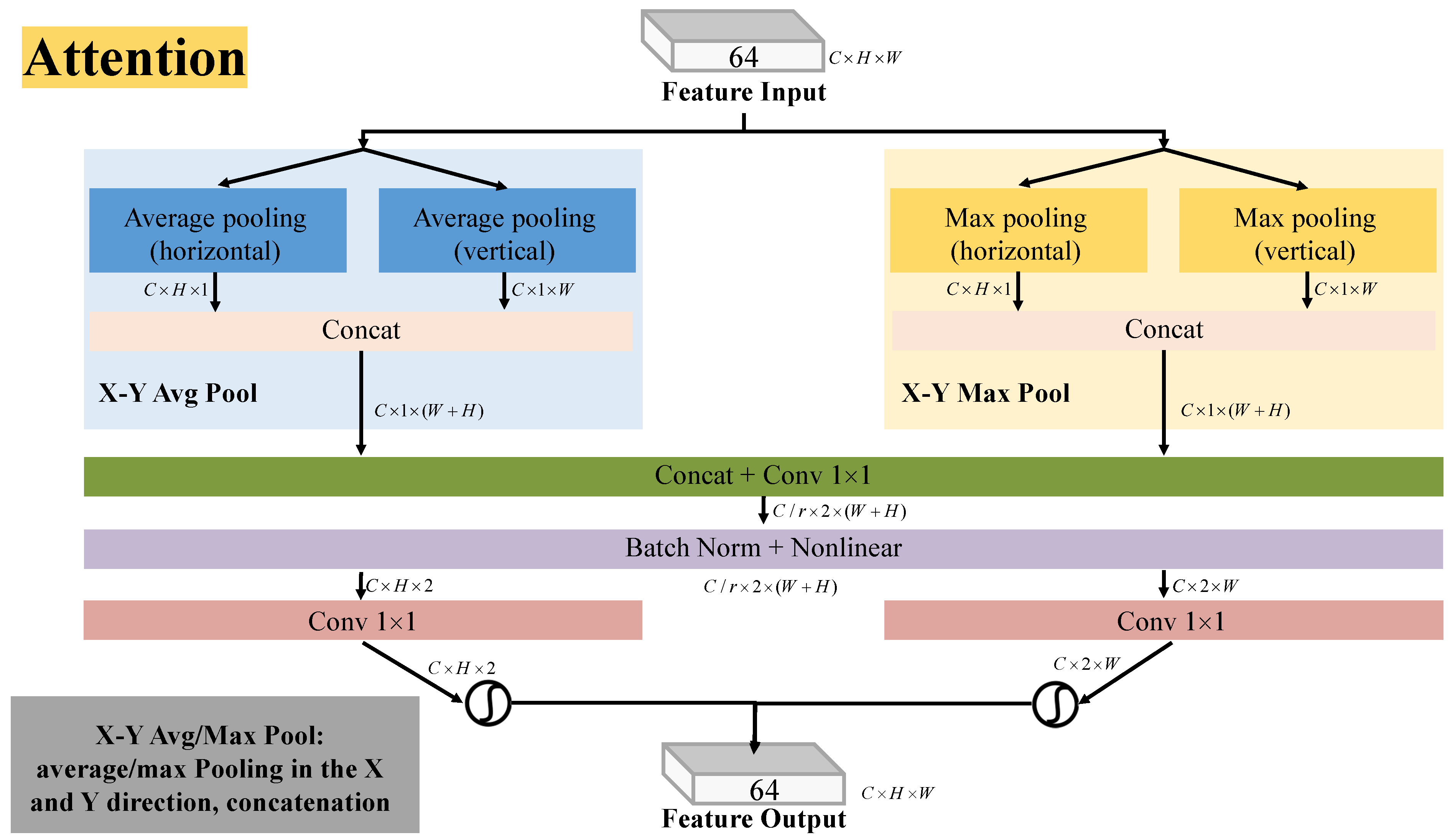
3.3. Multi-Scale Degradation-Representation-Guided Deblurring (Reblurring) Subnetwork

As shown in Figure 3, the multi-scale degradation-representation-guided reblurring and deblurring subnetworks share the same network structure but they do not share weights. For better illustration, this structure is subsequently referred to as the multi-scale degradation-guided reconstruction subnetwork. Following the design of the high-dimensional non-blind denoising (HDNBD) engine in [25], the multi-scale degradation-guided reconstruction sub-network adopts a U-net-based codec structure and follows core modules such as the feature enhancement module, enhanced residual bridge connection and attention module. DWT and IDWT are also used as down-sampling and up-samping methods, respectively. What is different is that the multi-scale degradation-guided reconstruction subnetwork takes both the image (sharp image x or blurred image y) and degradation representation E as input. Moreover, our design uses a multi-scale degradation representation fusion module for a better use of degradation representations.

At the encoding end, the input of each layer first goes through a feature enhancement module to initially extract features, and then the dimension is halved after DWT down-sampling as the input of the next layer. Both the encoding end and the decoding end are five layers in depth. The bottom layer of the encoding end goes through one Conv $3\times 3$ and ReLU to become the bottom layer of the decoder. Apart from the bottom layer, the input of each layer at the decoder end is the concatenation of the up-sampling value of the lower layer and the output of the multi-scale degradation representation block and the enhanced residual bridge connection block cascaded with it. After concatenation, the decoder-side feature is cascaded through a Conv $1\times 1$ and a feature enhancement module, and then the input is up-sampled to the upper layer.

The encoder side and the decoder side are set up with a jump connection section. The jump connection part of each layer consists of a feature enhancement module, the first enhanced residual bridge connection, the multi-scale degradation representation fusion module, and the second enhanced residual bridge connection cascade in turn. In particular, it should be noted that the input of the multi-scale degradation representation fusion module is not only the encoder-side features of that layer, but also the encoder-side features of the remaining layers and the implicit degradation representation E. The code-side features of each subsequent layer are denoted as $R_i$ subsequently, where i refers to the number of code-decoder layers, which increases from top to bottom. According to Figure 3, the dimensionality of E and $R_i$ is shown as

$$\begin{array}{cc}\hfill & E\in {\mathbb{R}}^{64\times H\times W}\hfill \\ \hfill & R_i\in {\mathbb{R}}^{64\times H_i\times W_i}i=1,\dots ,4\hfill \end{array}$$

(6)

where H and W denote the height and width of the input image, respectively. At the top layer (i.e., the layer with $i=1$), the output decoder-side feature after the feature enhancement module is again changed back to 64 channels after being passed through a Conv $1\times 1$, which is then passed through a Conv $3\times 3$ and then used as the input of the attention module. The output of the attention module is added element-wise to the features initially inputted at the encoder side, which is used as a global short connection to further enhance feature fusion between the encoder and decoder. Finally, the output image is obtained after one more Conv $1\times 1$: if the input image is x, the corresponding output is the reblurred image $y_{re}$, and the deblurred image $y_{de}$ is obtained when inputting the blurred image y. The structure of the sub-modules is analyzed below.

The structure of the feature enhancement module is shown in Figure 4, which consists of four sets of cascaded blocks of the Conv $3\times 3$ layer and rectified linear unit (ReLU), jump connections, and one Conv $1\times 1$ layer. As in Figure 3, 64/256 indicates the number of channels. It should be emphasized that the residual skip connection (indicated by a dashed line in the figure) of the input feature only exists at the encoder end, which is caused by the different number of channels between the encoder and decoder ends (256 at the encoder end and only 64 at the decoder end).

Figure 5 shows the structure of the enhanced residual bridge connection. This module consists of a cascade of $N_i$ residual blocks and an attention module in the end. Each residual block consists of two Conv $3\times 3$ layers, one ReLU layer and concatenation. Since the network enters deeper layers when i increases, the number of differences between the encoder-side features and the decoder-side features decreases, and therefore the number of residual blocks required decreases. In this paper, $N_i$ is set as $N_i=4-i+1$, i.e., 4, 3, 2, and 1 residual blocks from top to bottom, respectively.

The structure of the attention module is illustrated in Figure 6. Inspired by [25], the X–Y avg/max pool is designed to extract features in two different dimensions (vertical and horizontal directions). In more detail, the features are input and divided into two paths in the X–Y Avg Pool and X–Y Max Pool, followed by the average/max pooling of X (horizontal direction) and Y (vertical direction) in two modules, respectively, and then output via Concat operation. Afterwards, the average pooled and max pooled features are concatenated together again, and then partitioned after the Conv $1\times 1$ layer, BN (batch normalization) layer and nonlinear layer; finally, the reweighted output is obtained through a Sigmoid function.

Figure 7 shows the structure of the multi-scale degradation representation fusion block. Inputs that do not belong to the specific layer are denoted as the inputs of complementary layers. For instance, the complementary layers of the third layer are the first, second and fourth layer. As mentioned in Equation (6) above, the dimensionality of the encoder-side features $R_i$ of this layer and the implicit degradation representation E are not necessarily the same, so the inputs of the implicit degradation representation E need to go through interpolation down-sampling and ReLU first. The inputs of the complementary layers also need to be scale-transformed accordingly. In summary, the feature inputs of the upper and lower layers need to go through down-sampling/up-sampling, Conv $3\times 3$, and ReLU, respectively. Scale-transformed E and $R_i$ share the same dimensions of $64\times H_i\times W_i$. Afterwards, they are concatenated together by the Concat operation and fed into enhanced residual bridge connection after a Conv $1\times 1$ to reduce the number of channels to 64, thus obtaining the corresponding $R_i^{\prime }$ at the decoder end.

In summary, with the design of a high-dimensional reconstruction subnetwork detailed above, not only are the features of the input image itself efficiently extracted and fused with the decoder-side features, but also the implicit degradation representation E is incorporated into the obtained image features in various dimensions and utilized several times. The pseudo-code of the entire proposed method is shown in Algorithm 1.

Algorithm 1: The Overall Process of ${\mathrm{IDR}}^2\mathrm{ENet}$
	Data: Real Blurred Image y and the corresponding Real Sharp Image x
	Result: Reblurred image $y_{re}$ and deblurred image $x_{de}$
1	Initialization: Set learning rate, batch size and hyperparameters of the Adam
	solver; Cropping images from datasets;
2	while Training do
3			Expand and Crop the real blurred image y and corresponding sharp image x
			from the training dataset——Gopro;
4			Obtain the implicit degradation representations E using the degradation
			estimation network in Figure 2;
5			Input x and E into multi-scale reblurring subnetwork in Figure 7 to obtain
			reblurred image $y_{re}$;
6			Calculate ${\mathcal{L}}_{re}$ using Equation (7);
7			Input y and E into multi-scale deblurring subnetwork in Figure 7 to obtain
			deblurred image $x_{de}$;
8			Calculate ${\mathcal{L}}_{de}$ using Equation (9);
9			Evaluate total loss using Equation (11);
10			Back propagation and update the network parameters;
11	end
12	Obtain the reblurred image $y_{re}$ and deblurred image $x_{de}$;
13	Obtain the test image pairs from the test dataset——RWBI or RealBlur;
14	while Testing do
15			Extract the real blurred image y from the testing dataset;
16			Obtain the implicit degradation representations E using the degradation
			estimation network in Figure 2;
17			Input y and E into multi-scale deblurring subnetwork in Figure 7 to obtain
			deblurred image $x_{de}$;
18	end

3.4. Loss Function

In order to constrain the similarity between the reblurred image $y_{re}$ obtained by the reblurring process and the original real blurred image y so that they are as consistent as possible, this paper not only uses the ${\mathcal{L}}_2$ loss function to constrain the similarity at the low-level pixel level, but also uses the perceptual loss function to constrain the similarity of the high-level abstract features. Specifically, for the reblurring process, the loss function ${\mathcal{L}}_{re}$ is defined as follows:

$$\left\{\begin{array}{c}{\mathcal{L}}_2={∥y-y_{re}∥}_2^2\hfill \\ {\mathcal{L}}_{per}=perceptual(y,y_{re})\hfill \\ {\mathcal{L}}_{re}={\mathcal{L}}_2+{\mathcal{L}}_{per}\hfill \end{array}\right.$$

(7)

where $perceptual(·)$ is the perceptual loss function [34], expressed as

$${\mathcal{L}}_{per}={\displaystyle \frac{1}{WHC}}\sqrt{\sum _{x=1}^W\sum _{y=1}^H\sum _{c=1}^C{({\Phi }_{x,y,c}^l\left(y\right)-{\Phi }_{x,y,c}^l\left(y_{re}\right))}^2}$$

(8)

where ${\Phi }_{x,y,c}^l(·)$ denotes the output features of the classifier network from the l-th layer, C is the number of channels in the l-th layer, and W and H denote the width and height of the image, respectively. Instead of directly comparing the values of each pixel, the perceptual loss function compares the differences in the high-level feature space, as in deep networks trained for classification tasks (e.g., VGG19 [35]). For the deblurring process, apart from using the ${\mathcal{L}}_2$ loss function to calculate the difference in pixel values between the deblurred image $x_{de}$ and real sharp image x, the Structural SIMilarity (SSIM) loss function is used to calculate differences in structure, using the loss function ${\mathcal{L}}_{de}$ as follows:

$$\left\{\begin{array}{c}{\mathcal{L}}_2={∥x-x_{de}∥}_2^2\hfill \\ {\mathcal{L}}_{\mathrm{ssim}}=1-ssim(x,x_{de})\hfill \\ {\mathcal{L}}_{de}={\mathcal{L}}_2+{\mathcal{L}}_{\mathrm{ssim}}\hfill \end{array}\right.$$

(9)

where $ssim(·)$ refers to the SSIM loss function [36], with the expression shown as

$$ssim(x,y)={\displaystyle \frac{(2{\mu }_x{\mu }_y+C_1)(2{\sigma }_{xy}+C_2)}{({\mu }_x^2{\mu }_y^2+C_1)({\sigma }_x^2{\sigma }_y^2+C_2)}}$$

(10)

where ${\mu }_x$ and ${\mu }_y$ denote the mean value of image x and y, respectively, ${\sigma }_x^2$ and ${\sigma }_y^2$ denote the variance of image x and y, respectively, ${\sigma }_{xy}$ is the covariance between the two, and $C_1$ and $C_2$ are very small constants used to maintain stability. In summary, the loss function used by ${\mathrm{IDR}}^2\mathrm{ENet}$ is

$${\mathcal{L}}_{{\mathrm{IDR}}^2\mathrm{ENet}}=\lambda {\mathcal{L}}_{re}+{\mathcal{L}}_{de}$$

(11)

where $\lambda$ denotes the regularization factor between ${\mathcal{L}}_{re}$ and ${\mathcal{L}}_{de}$.

4. Experiments

4.1. Datasets

The datasets used in this paper include the GoPro dataset [8], the RealBlur dataset [37], and the RWBI dataset [31].

The GoPro dataset is commonly used for training and evaluating deep-learning-based deblurring methods, which is produced from clear videos captured at 240 fps (frames per second) using the GoPro Hero4 Black camera, and the blurred images are obtained by averaging sharp videos over time windows of different durations, which correspond to the sharp images in the center of the time window. The GoPro dataset consists of 2103 pairs of blurred and sharp images for training and 1111 pairs of images for testing. In this paper, the GoPro dataset is applied to the training of ${\mathrm{IDR}}^2\mathrm{ENet}$.

The RealBlur dataset, produced by Rim et al. [37], contains paired real blurred images and consists of two subsets with the same image content, RealBlur-J and RealBlur-R. RealBlur-R is generated from raw camera images (RAW images) and RealBlur-J is generated from JPEG images processed by the camera ISP. Each subset contains 4738 pairs of blurred and corresponding real sharp images from 232 different low-light static scenes, of which 3758 pairs are used for training and 980 pairs are used for testing. In this paper, the RealBlur dataset is applied to the testing of ${\mathrm{IDR}}^2\mathrm{ENet}$.

The RWBI dataset contains 3112 real blurred images from 22 different scenes. These blurred images were obtained from a variety of mobile devices, including Huawei P30 Pro, Samsung S9 Plus, iPhone XS, and GoPro Hero5 Black cameras. However, it is worth mentioning that the RWBI dataset only contains real blurred images without the corresponding sharp images. Therefore, the RWBI dataset is only for the testing of ${\mathrm{IDR}}^2\mathrm{ENet}$ in this paper.

4.2. Training Settings

${\mathrm{IDR}}^2\mathrm{ENet}$ proposed in this paper is implemented on PyTorch, and all experiments are executed on an NVIDIA GeForce GTX 2080Ti GPU. During training, images in the GoPro dataset are randomly flipped and rotated horizontally during data expansion, and then are further cropped into patches of size $256\times 256$, with the batch size set to 2. We use the Adam solver as the optimizer for ${\mathrm{IDR}}^2\mathrm{ENet}$ with hyperparameters set to ${\beta }_1=0.9$, ${\beta }_2=0.99$, and $ϵ={10}^{-8}$. The learning rate $\gamma$ is initially set as ${10}^{-4}$ and decreased to ${10}^{-6}$ when training stops.

5. Results and Analysis

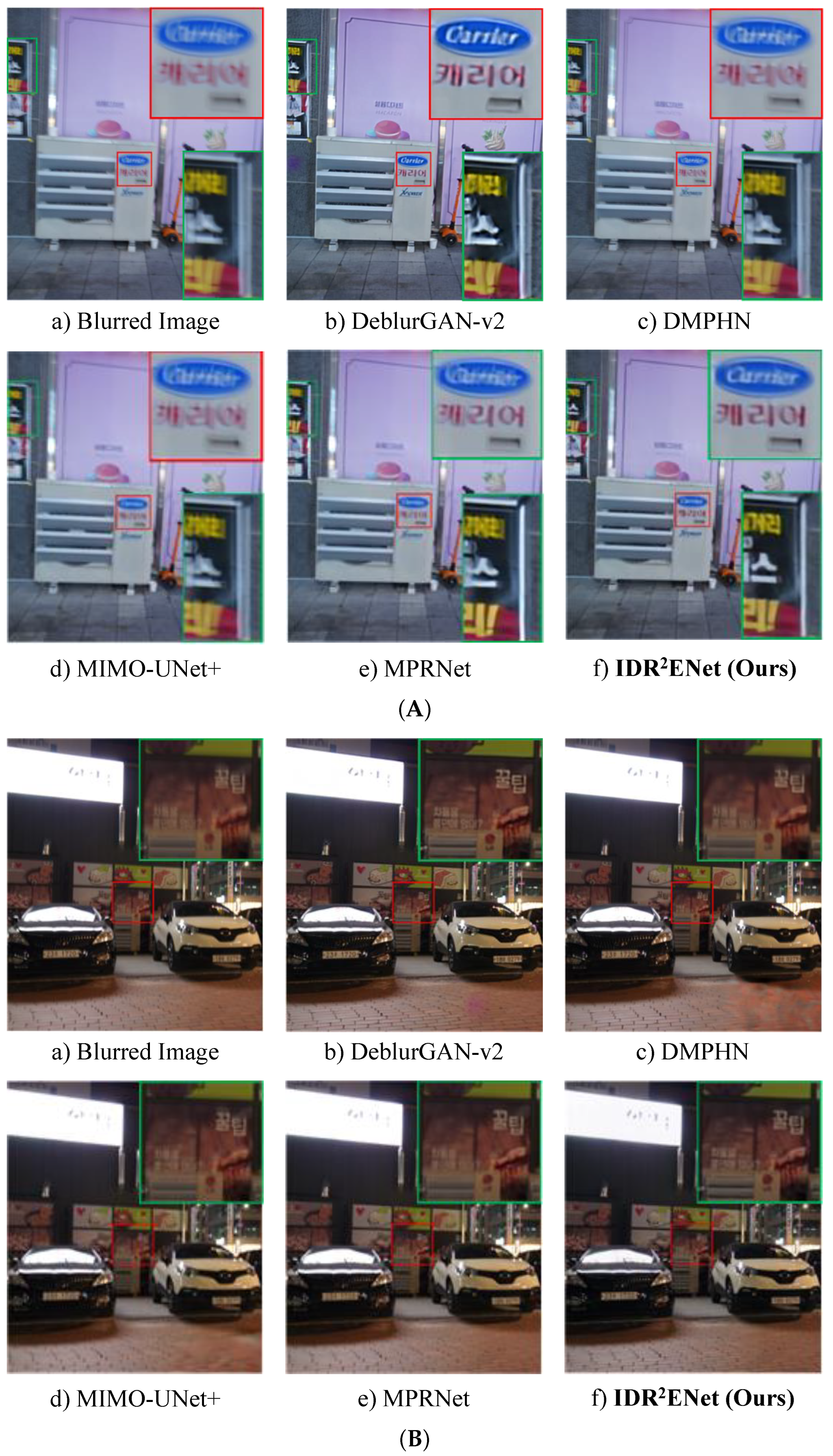
5.1. Real Image Deblurring

To evaluate the performance of ${\mathrm{IDR}}^2\mathrm{ENet}$, traditional methods such as those proposed by Xu et al. [6], Hu et al. [21], and Pan et al. [38], as well as deep-learning-based methods such as SRN [9], SVRNN [39], DeepDeblur [8], DeblurGAN [10], DMPHN [40], DeblurGAN-v2 [16], DBGAN [31], MIMO-Unet [41], MIMO-Unet+ [41], MPRNet [42], and Lightweight MIMO-WNet [43], are introduced in this paper for comparison.

We first tested the objective metric PSNR/SSIM results of each deblurring method on the real blur datasets RealBlur-J and RealBlur-R, which are shown in

Table 1. Comparison of PSNR/SSIM for different methods on RealBlur-J and RealBlur-R.

Type	Method	RealBlur-J		RealBlur-R
		PSNR (dB)	SSIM	PSNR (dB)	SSIM
Traditional	Xu et al. [6]	27.14	0.830	34.46	0.937
	Hu et al. [21]	26.41	0.803	33.67	0.916
	Pan et al. [38]	27.22	0.790	34.01	0.917
Deep-Learning-Based	SRN [9]	28.56	0.867	35.66	0.947
	SVRNN [39]	27.80	0.847	35.48	0.945
	DeepDeblur [8]	27.87	0.827	32.51	0.841
	DeblurGAN [10]	27.97	0.834	33.79	0.903
	DMPHN [40]	28.42	0.860	35.70	0.948
	DeblurGAN-V2 [16]	28.70	0.867	35.26	0.944
	DBGAN [31]	24.93	0.745	33.78	0.909
	MIMO-Unet [41]	27.76	0.836	35.47	0.946
	MIMO-Unet+ [41]	27.63	0.837	35.54	0.947
	MPRNet [42]	28.70	0.873	35.99	0.952
	Lightweight MIMO-WNet [43]	28.52	0.865	35.76	0.950
	${\mathrm{IDR}}^2\mathrm{ENet}$ (Ours)	28.81	0.876	35.96	0.952

, respectively.

As seen in Table 1, the ${\mathrm{IDR}}^2\mathrm{ENet}$ approach proposed in this paper obtains superior results on both the RealBlur-J and RealBlur-R datasets. The PSNR and SSIM of traditional methods lag behind those of most of the deep-learning-based methods, the results of which are lower on both the RealBlur-J and RealBlur-R datasets, which indicates that the traditional-based method models deblurring as a specific mathematical process that cannot cope with the complex degradation in real blurred images and does not work well. When compared to deep learning-based methods, ${\mathrm{IDR}}^2\mathrm{ENet}$ shows some improvement in effectiveness, such as an objective metric increase of 0.11 dB/0.003 in the RealBlur-J dataset compared to the newer MPRNet.

Furthermore, Figure 8A,B show the deblurred visual performances of different methods on two real blurred images from the Reblur-J dataset.

In Figure 8A, it can be seen that the blurred image suffers from severe blur degradation. The image reconstructed by DeblurGAN-v2 achieves some deblurring effect. However, compared with the results of ${\mathrm{IDR}}^2\mathrm{ENet}$, the reblurred image recovered by DeblurGAN-v2 still retains blur artifacts and a purple-red artifact on the wall from the poster on the left side, and the reblurred image of ${\mathrm{IDR}}^2\mathrm{ENet}$ is clearer and sharper.

From the enlarged font blocks, the deblurred results of DeblurGAN-v2 are sharper, but still have slight artifacts at the edges of the font, while the results of ${\mathrm{IDR}}^2\mathrm{ENet}$ do not. When compared with other comparison algorithms, ${\mathrm{IDR}}^2\mathrm{ENet}$ recovered sharper results in the poster and font parts. Compared with Figure 8A, the blurred image of Figure 8B has milder blur degradation. The results of DeblurGAN-v2, DMPHN, and MIMO-UNet+ all show varying degrees of mottled artifacts in the ground portion of the lower right corner of the deblurred image when viewed overall. From the enlarged blocks, ${\mathrm{IDR}}^2\mathrm{ENet}$ still obtains reconstructed results with clearer details. In general, deblurred images of ${\mathrm{IDR}}^2\mathrm{ENet}$ reconstruct the details more clearly and do not generate incorrect artifacts.

Furthermore, in order to further verify the effectiveness of ${\mathrm{IDR}}^2\mathrm{ENet}$ on real image deblurring tasks, we tested it on the RWBI dataset. Two images were selected and their visual effects before and after processing are shown in Figure 9 and Figure 10, respectively.

In Figure 9, the real blurred image after ${\mathrm{IDR}}^2\mathrm{ENet}$ processing achieves a good deblurring performance, e.g., the edges of the building at the center of real blurred image and the logo on top of it are very clear and do not have any vignettes. However, there still exist some areas where the deblurring performance is not satisfactory, such as tree branches on the right side of the image. In Figure 10, the real blurred image after ${\mathrm{IDR}}^2\mathrm{ENet}$ deblurring is clearly identifiable in the enlarged text part of the letters. Overall, the test results on the RealBlur and RWBI datasets show that ${\mathrm{IDR}}^2\mathrm{ENet}$ is consistently effective and reliable in real image deblurring tasks.

Moreover, the author captured some real blurred images using a mobile phone and processed them using ${\mathrm{IDR}}^2\mathrm{ENet}$, and the comparative results are shown in Figure 11.

From Figure 11, we can see that the deblurred images after ${\mathrm{IDR}}^2\mathrm{ENet}$ processing no longer have obvious blurred parts in the overall perception, and the text that is most affected by the blur degradation is basically recovered.

As a complementary experiment, we also select a low-contrast image from the RealBlur-J dataset to test ${\mathrm{IDR}}^2\mathrm{ENet}$’s performance in low-contrast situations, with the results shown in Figure 12. The results show that our ${\mathrm{IDR}}^2\mathrm{ENet}$ also performs well on low-contrast blurred images.

5.2. Network Complexity Analysis

Table 2. Comparison of network complexity of different methods.

Methods	Parameters	FLOPs	Time	RealBlur-J
				PSNR (dB)	SSIM
DMPHN [40]	21.7 M	678.56 G	0.034 s	28.42	0.86
DeblurGAN-v2 [16]	60.9 M	411.34 G	0.082 s	28.7	0.867
DBGAN [31]	11.6 M	660.20 G	0.084 s	24.93	0.745
MIMO-Unet+ [41]	16.1 M	154.24 G	0.032 s	27.63	0.837
MPRNet [42]	20.1 M	760.11 G	0.077 s	28.7	0.876
Lightweight MIMO-WNet [43]	14.1 M	138.81 G	0.028 s	28.52	0.865
${\mathrm{IDR}}^2\mathrm{ENet}$ (Ours) Training	13.4 M	317.91 G	-	-	-
${\mathrm{IDR}}^2\mathrm{ENet}$ (Ours) Testing	7.5 M	169.78 G	0.012 s	28.81	0.876

shows the number of network parameters, running time and FLOPs of different methods, where FLOPs are calculated on $256\times 256$ image blocks, the running time is calculated on the average processing time over 100 blur images, and the deblurring performance of each method on the RealBlur-J dataset is listed for comparison at the same time. Note that all experiments are executed on an NVIDIA GeForce GTX 2080Ti GPU.As shown in Table 2, ${\mathrm{IDR}}^2\mathrm{ENet}$ has 13.4 M parameters and 317.91 G FLOPs during training, while it has 7.5 M counts and 169.78 G FLOPs during testing, which has a smaller memory footprint because no reblurring process is involved during testing. Compared with most methods, ${\mathrm{IDR}}^2\mathrm{ENet}$ has a greater advantage in terms of the number of parameters and FLOPs because it does not involve iterations and other complicated designs. Although the FLOPs of MIMO-UNet+ [41] are slightly smaller than those of this paper with a difference of 15.54 G (compared to the FLOPs during testing), it still has twice the number of parameters of ${\mathrm{IDR}}^2\mathrm{ENet}$. Lightweight MIMO-Wnet [43] has smaller FLOPs by improving a lightweight structure of MIMO-UNet [41]. Although its deblurring effect is somewhat improved compared to the latter, it is still lower than ${\mathrm{IDR}}^2\mathrm{ENet}$’s performance. For the running time, ${\mathrm{IDR}}^2\mathrm{ENet}$ requires less time than any other network, as shown in Table 2. In general, compared with other methods, ${\mathrm{IDR}}^2\mathrm{ENet}$ ensures excellent deblurring performance while keeping the network complexity to a smaller level.

5.3. Ablation Study

5.3.1. Validation of the Effectiveness of Implicit Degradation Representations-Guided Reconstruction

Implicit degradation representation E estimated by the degradation estimation subnetwork guides the reconstruction of blurred images by the deblurring process. In order to verify the contribution of implicit degradation representation E to the final deblurring performance, ablation studies are designed in this paper. Specifically, only the deblurring process is retained on the original network framework of ${\mathrm{IDR}}^2\mathrm{ENet}$, and the high-dimensional deblurring subnetwork is made to take only real blurred image as input, at which time the network framework is shown in Figure 13. This is noted as ${\mathrm{IDR}}^2\mathrm{ENet}$-Q. The results of retraining on the GoPro dataset with exactly the same experimental settings as ${\mathrm{IDR}}^2\mathrm{ENet}$ are shown in

Table 3. Comparison of the performance of different network structures.

Network Framework	RealBlur-J
	PSNR (dB)	SSIM
${\mathrm{IDR}}^2\mathrm{ENet}$-Q	28.4	0.863
${\mathrm{IDR}}^2\mathrm{ENet}$-R	28.64	0.87
${\mathrm{IDR}}^2\mathrm{ENet}$	28.81	0.875

.

As shown in Table 3, the performance of ${\mathrm{IDR}}^2\mathrm{ENet}$-Q is reduced by 0.41 dB/0.012 compared to the original ${\mathrm{IDR}}^2\mathrm{ENet}$, which proves that ${\mathrm{IDR}}^2\mathrm{ENet}$ can better reconstruct deblurred images and achieve a higher performance guided by the implicit degradation representation E when facing complex degradation in real blurred images.

5.3.2. Validation of Reblurring Process

The proposed ${\mathrm{IDR}}^2\mathrm{ENet}$ employs a reblurring process to help the degradation estimation subnetwork to better estimate the implicit degradation representation E. Thus, an ablation experiment is designed to verify it in this section. Specifically, the network framework with the reblurring process removed and only the degradation estimation process and deblurring process retained is shown in Figure 14. This framework is denoted as ${\mathrm{IDR}}^2\mathrm{ENet}$-R, which is also retrained on exactly the same experimental settings. The deblurring results of ${\mathrm{IDR}}^2\mathrm{ENet}$-R on the RealBlur-J dataset are also shown in Table 3. In Table 3, the result of ${\mathrm{IDR}}^2\mathrm{ENet}$-R is 28.64 dB/0.870, which is a decrease of 0.17 dB/0.005 compared to the original ${\mathrm{IDR}}^2\mathrm{ENet}$. This proves that the degradation estimation subnetwork can better estimate the implicit degradation representations in real blurred images through the reblurring process, which in turn better helps the reconstruction process.

5.4. Discussion

We perform five experiments in this section, including (1) ${\mathrm{IDR}}^2\mathrm{ENet}$’s performance on the real blur datasets RealBlur (Table 1 and Figure 8) and RWBI (Figure 9 and Figure 10), (2) ${\mathrm{IDR}}^2\mathrm{ENet}$’s performance on real captured blur images (Figure 11), (3) ${\mathrm{IDR}}^2\mathrm{ENet}$’s performance on low-contrast blur images (Figure 12), (4) a comparison of ${\mathrm{IDR}}^2\mathrm{ENet}$’s complexity and running time with other networks (Table 2), and (5) ablation experiments to verify the role of the degradation estimation subnetwork and reblurring subnetwork of ${\mathrm{IDR}}^2\mathrm{ENet}$ (Figure 13 and Figure 14, and Table 3). The overall results show that our ${\mathrm{IDR}}^2\mathrm{ENet}$ not only achieves good performance on various kinds of real blurred images, but it also has a smaller network complexity as well as better quantitative metrics, known as PSNR and SSIM. The results of the ablation study also demonstrate the effectiveness of our methods—reblur estimation and degradation estimation.

However, there are still areas where our results can be improved. For example, the deblurring effect of ${\mathrm{IDR}}^2\mathrm{ENet}$ on real captured blurred images (Figure 11) can still be enhanced, which proves that the network’s understanding of degradation representations in blurred images is perhaps not sufficient. Therefore, it might be useful to consider introducing GAN-based structures in the design of the degradation estimation subnetwork and reblurring network to enhance the understanding, constraint and utilization of degradation representations.

6. Conclusions

In this paper, we propose a real image deblurring network framework, ${\mathrm{IDR}}^2\mathrm{ENet}$, based on reblurring to estimate the implicit degradation representation. Unlike the general methods for estimating explicit degradation representations, ${\mathrm{IDR}}^2\mathrm{ENet}$ learns implicit degradation representations by constructing a “sharp image–blurred image” reblurring process, and uses the generated degradation representations to guide the deblurring and reblurring processes. In order to better constrain the feature similarity between the reblurred image and the original blurred image, a perceptual loss function is added to the corresponding loss function, and SSIM is introduced to calculate the difference between the deblurred image and the original blurred image. The experimental results show that our network achieves stable and efficient deblurring results for real image deblurring on the RealBlur dataset, RWBI dataset and real captured blurred images. Additionally, ${\mathrm{IDR}}^2\mathrm{ENet}$ has better results and lower network complexity compared with other methods.

References

1. Zhang, K.; Ren, W.; Luo, W.; Lai, W.S.; Stenger, B.; Yang, M.H.; Li, H. Deep image deblurring: A survey. Int. J. Comput. Vis. 2022, 130, 2103–2130. [Google Scholar] [CrossRef]
2. Michaeli, T.; Irani, M. Blind deblurring using internal patch recurrence. In Proceedings of the Computer Vision–ECCV 2014: 13th European Conference, Zurich, Switzerland, 6–12 September 2014; Proceedings, Part III 13. Springer: Berlin/Heidelberg, Germany, 2014; pp. 783–798. [Google Scholar]
3. Krishnan, D.; Fergus, R. Fast image deconvolution using hyper-Laplacian priors. In Proceedings of the 22nd International Conference on Neural Information Processing Systems (NIPS’ 09), Vancouver, BC, Canada, 7–10 December 2009; Curran Associates Inc.: Red Hook, NY, USA, 2009; pp. 1033–1041. [Google Scholar]
4. Fergus, R.; Singh, B.; Hertzmann, A.; Roweis, S.T.; Freeman, W.T. Removing camera shake from a single photograph. In Acm Siggraph 2006 Papers; ACM: New York, NY, USA, 2006; pp. 787–794. [Google Scholar]
5. Chan, T.F.; Wong, C.K. Total variation blind deconvolution. IEEE Trans. Image Process. 1998, 7, 370–375. [Google Scholar] [CrossRef] [PubMed] [Green Version]
6. Xu, L.; Zheng, S.; Jia, J. Unnatural l0 sparse representation for natural image deblurring. In Proceedings of the IEEE Conference on Computer Vision and Pattern Recognition, Portland, OR, USA, 23–28 June 2013; pp. 1107–1114. [Google Scholar]
7. Cho, S.; Lee, S. Fast Motion Deblurring. ACM Trans. Graph. 2009, 28, 145:1–145:8. [Google Scholar] [CrossRef]
8. Nah, S.; Hyun Kim, T.; Mu Lee, K. Deep multi-scale convolutional neural network for dynamic scene deblurring. In Proceedings of the IEEE Conference on Computer Vision and Pattern Recognition, Honolulu, HI, USA, 21–26 July 2017; pp. 3883–3891. [Google Scholar]
9. Tao, X.; Gao, H.; Shen, X.; Wang, J.; Jia, J. Scale-recurrent network for deep image deblurring. In Proceedings of the IEEE Conference on Computer Vision and Pattern Recognition, Salt Lake City, UT, USA, 18–23 June 2018; pp. 8174–8182. [Google Scholar]
10. Kupyn, O.; Budzan, V.; Mykhailych, M.; Mishkin, D.; Matas, J. Deblurgan: Blind motion deblurring using conditional adversarial networks. In Proceedings of the IEEE Conference on Computer Vision and Pattern Recognition, Salt Lake City, UT, USA, 18–23 June 2018; pp. 8183–8192. [Google Scholar]
11. Schuler, C.J.; Hirsch, M.; Harmeling, S.; Schölkopf, B. Learning to Deblur. arXiv 2014, arXiv:1406.7444. [Google Scholar] [CrossRef] [PubMed]
12. Hradiš, M.; Kotera, J.; Zemčík, P.; Šroubek, F. Convolutional Neural Networks for Direct Text Deblurring. In Proceedings of the British Machine Vision Conference (BMVC), Swansea, UK, 7–10 September 2015; Xie, X., Jones, M.W., Tam, G.K.L., Eds.; BMVA Press: Durham, UK, 2015; pp. 6.1–6.13. [Google Scholar] [CrossRef] [Green Version]
13. Ren, D.; Zhang, K.; Wang, Q.; Hu, Q.; Zuo, W. Neural Blind Deconvolution Using Deep Priors. arXiv 2020, arXiv:1908.02197. [Google Scholar]
14. Sun, J.; Cao, W.; Xu, Z.; Ponce, J. Learning a Convolutional Neural Network for Non-uniform Motion Blur Removal. arXiv 2015, arXiv:1503.00593. [Google Scholar]
15. Chakrabarti, A. A Neural Approach to Blind Motion Deblurring. arXiv 2016, arXiv:1603.04771. [Google Scholar]
16. Kupyn, O.; Martyniuk, T.; Wu, J.; Wang, Z. Deblurgan-v2: Deblurring (orders-of-magnitude) faster and better. In Proceedings of the IEEE/CVF International Conference on Computer Vision, Seoul, Republic of Korea, 27 October–2 November 2019; pp. 8878–8887. [Google Scholar]
17. Nimisha, T.M.; Kumar Singh, A.; Rajagopalan, A.N. Blur-invariant deep learning for blind-deblurring. In Proceedings of the IEEE International Conference on Computer Vision, Venice, Italy, 22–29 October 2017; pp. 4752–4760. [Google Scholar]
18. Lu, B.; Chen, J.C.; Chellappa, R. Unsupervised Domain-Specific Deblurring via Disentangled Representations. arXiv 2019, arXiv:1903.01594. [Google Scholar]
19. Gao, H.; Tao, X.; Shen, X.; Jia, J. Dynamic scene deblurring with parameter selective sharing and nested skip connections. In Proceedings of the IEEE/CVF Conference on Computer Vision and Pattern Recognition, Long Beach, CA, USA, 15–20 June 2019; pp. 3848–3856. [Google Scholar]
20. Shen, Z.; Lai, W.S.; Xu, T.; Kautz, J.; Yang, M.H. Deep semantic face deblurring. In Proceedings of the IEEE Conference on Computer Vision and Pattern Recognition, Salt Lake City, UT, USA, 18–23 June 2018; pp. 8260–8269. [Google Scholar]
21. Hu, Z.; Cho, S.; Wang, J.; Yang, M.H. Deblurring low-light images with light streaks. In Proceedings of the IEEE Conference on Computer Vision and Pattern Recognition, Columbus, OH, USA, 23–28 June 2014; pp. 3382–3389. [Google Scholar]
22. Jolicoeur-Martineau, A. The relativistic discriminator: A key element missing from standard GAN. arXiv 2018, arXiv:1807.00734. [Google Scholar]
23. Dong, W.; Wang, P.; Yin, W.; Shi, G.; Wu, F.; Lu, X. Denoising prior driven deep neural network for image restoration. IEEE Trans. Pattern Anal. Mach. Intell. 2018, 41, 2305–2318. [Google Scholar] [CrossRef] [PubMed] [Green Version]
24. Zhai, S.; Ren, C.; Wang, Z.; He, X.; Qing, L. An effective deep network using target vector update modules for image restoration. Pattern Recognit. 2022, 122, 108333. [Google Scholar] [CrossRef]
25. Qin, M.; Ren, C.; Yang, H.; He, X.; Wang, Z. Blind Image Denoising via Deep Unfolding Network with Degradation Information Guidance. IEEE Trans. Circuits Syst. II Express Briefs 2023. [Google Scholar] [CrossRef]
26. Li, D.; Zhang, Y.; Cheung, K.C.; Wang, X.; Qin, H.; Li, H. Learning Degradation Representations for Image Deblurring. In Proceedings of the Computer Vision–ECCV 2022: 17th European Conference, Tel Aviv, Israel, 23–27 October 2022; Proceedings, Part XVIII. Springer: Berlin/Heidelberg, Germany, 2022; pp. 736–753. [Google Scholar]
27. Cannon, M. Blind deconvolution of spatially invariant image blurs with phase. IEEE Trans. Acoust. Speech Signal Process. 1976, 24, 58–63. [Google Scholar] [CrossRef]
28. Kundur, D.; Hatzinakos, D. Blind image deconvolution. IEEE Signal Process. Mag. 1996, 13, 43–64. [Google Scholar] [CrossRef] [Green Version]
29. Xu, L.; Jia, J. Two-phase kernel estimation for robust motion deblurring. In Proceedings of the Computer Vision–ECCV 2010: 11th European Conference on Computer Vision, Heraklion, Greece, 5–11 September 2010; Proceedings, Part I 11. Springer: Berlin/Heidelberg, Germany, 2010; pp. 157–170. [Google Scholar]
30. Bahat, Y.; Efrat, N.; Irani, M. Non-uniform blind deblurring by reblurring. In Proceedings of the IEEE International Conference on Computer Vision, Venice, Italy, 22–29 October 2017; pp. 3286–3294. [Google Scholar]
31. Zhang, K.; Luo, W.; Zhong, Y.; Ma, L.; Stenger, B.; Liu, W.; Li, H. Deblurring by realistic blurring. In Proceedings of the IEEE/CVF Conference on Computer Vision and Pattern Recognition, Seattle, WA, USA, 13–19 June 2020; pp. 2737–2746. [Google Scholar]
32. Chen, H.; Gu, J.; Gallo, O.; Liu, M.Y.; Veeraraghavan, A.; Kautz, J. Reblur2deblur: Deblurring videos via self-supervised learning. In Proceedings of the 2018 IEEE International Conference on Computational Photography (ICCP), Pittsburgh, PA, USA, 4–6 May 2018; pp. 1–9. [Google Scholar]
33. Wang, L.; Wang, Y.; Dong, X.; Xu, Q.; Yang, J.; An, W.; Guo, Y. Unsupervised degradation representation learning for blind super-resolution. In Proceedings of the IEEE/CVF Conference on Computer Vision and Pattern Recognition, Nashville, TN, USA, 20–25 June 2021; pp. 10581–10590. [Google Scholar]
34. Johnson, J.; Alahi, A.; Fei-Fei, L. Perceptual losses for real-time style transfer and super-resolution. In Proceedings of the Computer Vision–ECCV 2016: 14th European Conference, Amsterdam, The Netherlands, 11–14 October 2016; Proceedings, Part II 14. Springer: Berlin/Heidelberg, Germany, 2016; pp. 694–711. [Google Scholar]
35. Simonyan, K.; Zisserman, A. Very deep convolutional networks for large-scale image recognition. arXiv 2014, arXiv:1409.1556. [Google Scholar]
36. Wang, Z.; Simoncelli, E.P.; Bovik, A.C. Multiscale structural similarity for image quality assessment. In Proceedings of the IEEE Thrity-Seventh Asilomar Conference on Signals, Systems & Computers, Pacific Grove, CA, USA, 9–12 November 2003; Volume 2, pp. 1398–1402. [Google Scholar]
37. Rim, J.; Lee, H.; Won, J.; Cho, S. Real-world blur dataset for learning and benchmarking deblurring algorithms. In Proceedings of the Computer Vision–ECCV 2020: 16th European Conference, Glasgow, UK, 23–28 August 2020; Proceedings, Part XXV 16. Springer: Berlin/Heidelberg, Germany, 2020; pp. 184–201. [Google Scholar]
38. Pan, J.; Sun, D.; Pfister, H.; Yang, M.H. Blind image deblurring using dark channel prior. In Proceedings of the IEEE Conference on Computer Vision and Pattern Recognition, Las Vegas, NV, USA, 27–30 June 2016; pp. 1628–1636. [Google Scholar]
39. Zhang, J.; Pan, J.; Ren, J.; Song, Y.; Bao, L.; Lau, R.W.; Yang, M.H. Dynamic scene deblurring using spatially variant recurrent neural networks. In Proceedings of the IEEE Conference on Computer Vision and Pattern Recognition, Salt Lake City, UT, USA, 18–23 June 2018; pp. 2521–2529. [Google Scholar]
40. Zhang, H.; Dai, Y.; Li, H.; Koniusz, P. Deep stacked hierarchical multi-patch network for image deblurring. In Proceedings of the IEEE/CVF Conference on Computer Vision and Pattern Recognition, Long Beach, CA, USA, 15–20 June 2019; pp. 5978–5986. [Google Scholar]
41. Cho, S.J.; Ji, S.W.; Hong, J.P.; Jung, S.W.; Ko, S.J. Rethinking coarse-to-fine approach in single image deblurring. In Proceedings of the IEEE/CVF International Conference on Computer Vision, Montreal, QC, Canada, 11–17 October 2021; pp. 4641–4650. [Google Scholar]
42. Zamir, S.W.; Arora, A.; Khan, S.; Hayat, M.; Khan, F.S.; Yang, M.H.; Shao, L. Multi-stage progressive image restoration. In Proceedings of the IEEE/CVF Conference on Computer Vision and Pattern Recognition, Nashville, TN, USA, 20–25 June 2021; pp. 14821–14831. [Google Scholar]
43. Liu, M.; Yu, Y.; Li, Y.; Ji, Z.; Chen, W.; Peng, Y. Lightweight MIMO-WNet for single image deblurring. Neurocomputing 2023, 516, 106–114. [Google Scholar] [CrossRef]
Figure 1. Network structure of IDR 2 ENet , which is the Implicit Degradation Representations and Reblur Estimation Network for real image deblurring.
Applsci 13 07738 g001
Figure 2. Network structure of degradation estimation subnetwork.
Applsci 13 07738 g002
Figure 3. Network structure of multi-scale degradation-representation-guided deblurring (reblurring) subnetwork.
Applsci 13 07738 g003
Figure 4. Structure of the feature enhancement block.
Applsci 13 07738 g004
Figure 5. Structure of the enhanced residual bridge connection.
Applsci 13 07738 g005
Figure 6. Structure of attention.
Applsci 13 07738 g006
Figure 7. Structure of the multi-scale degradation representation fusion block.
Applsci 13 07738 g007
Figure 8. Deblurring performances of various methods on the RealBlur-J dataset. From left to right, top to bottom: (a) blurred image, (b) DeblurGAN-v2 [16], (c) DMPHN [40], (d) MIMO-UNet+ [41], (e) MPRNet [42], (f) IDR 2 ENet (Ours). (A) Deblurring performance: Image-1. (B) Deblurring performance: Image-2.
Applsci 13 07738 g008
Figure 9. Deblurring performances of IDR 2 ENet on the RWBI dataset—Image 1.
Applsci 13 07738 g009
Figure 10. Deblurring performances of IDR 2 ENet on the RWBI Dataset—Image 2.
Applsci 13 07738 g010
Figure 11. Deblurring performances of IDR 2 ENet on images captured by a mobile phone. From left to right: real blur images, and deblurred images of IDR 2 ENet .
Applsci 13 07738 g011
Figure 12. Deblurring performances of IDR 2 ENet on low-contrast images from RealBlur-J. From left to right: (a) the low-contrast blur image, and (b) the corresponding deblurred image of IDR 2 ENet .
Applsci 13 07738 g012
Figure 13. Network structure of IDR 2 ENet -Q.
Applsci 13 07738 g013
Figure 14. Network structure of IDR 2 ENet -R.
Applsci 13 07738 g014