Improved Detector Based on Yolov5 for Typical Targets on the Sea Surfaces

Abstract

Detection of targets on sea surfaces is an important area of application that can bring great benefits to the management and control systems in marine environments. However, there are few open-source datasets accessible for the purpose of object detection on seas and rivers. In this paper, a study is conducted on the improved detection algorithms based on the YOLOv5 model. The dataset for the tests contains ten categories of typical objects that are commonly seen in the contexts of seas, including ships, devices, and structures. Multiple augmentation methods are employed in the pre-processing of the input data, which are verified to be effective in enhancing the generalization ability of the algorithm. Moreover, a new form of the loss function is proposed that highlights the effects of the high-quality boxes during training. The results demonstrate that the adapted loss function contributes to a boost in the model performance. According to the ablation studies, the synthesized methods raise the inference accuracy by making up for several shortcomings of the baseline model for the detection tasks of single or multiple targets from varying backgrounds.

1. Introduction

With the rapid development of marine technology in recent years, the detection of objects in sea and ocean environments has become an increasingly crucial area of research and application. Intelligent systems that can recognize targets with little use of manpower have been playing a vital role in harbor management, navigation, ship rescue, collision prevention, and so on [1]. Situations with targets of a variety of categories and sizes under different weather and optical conditions must be dealt with, which places high requirements on the system in recognition and decision-making at a sufficient precision under different circumstances. However, the scarcity of maritime target datasets hinders the progress of study in this area.

Object detection algorithms in computer vision that can be employed in marine applications can be divided into traditional methods and deep-learning-based ones, with the latter being widely implemented and improved recently for detection and recognition tasks [2,3,4]. One of the typical two-stage detection algorithms is R-CNN [5], which tackled the problems of classification and localization in two steps, i.e., generating region proposals that potentially contain objects with the selective search algorithm and then performing feature extraction using the convolutional neural networks. This algorithm was further modified and enhanced with variants such as Fast R-CNN [6] and Faster R-CNN [7] that surpassed the original algorithm in model performance. Other two-stage detectors, such as R-FCN [8], Cascade R-CNN [9], and Mask R-CNN [10] extended on the basis of R-CNN or its variant, can also gain remarkable performance in object detection tasks. Single-stage algorithms such as the You-Only-Look-Once (YOLO) series [11,12], single-shot multi-box detector (SSD) [13], and RetinaNet [14] can usually run at much higher speeds at inference. YOLOv1 [11] provided unified training for classification and localization, reaching an inference speed of 45 fps (much faster than Faster R-CNN) and a mean average precision (mAP) score of 63.4% (comparable to Faster R-CNN (ZF version)) evaluated on the PASCAL VOC [15] 2007 and 2012 datasets. Later, modifications were made to this original algorithm that led to the generation of several follow-up versions (YOLOv2 to YOLOv5). YOLOv5 was released shortly after YOLOv4, with model sizes that were significantly reduced and a faster training speed compared with the latter. Models with different scales of the network can be selected, including YOLOv5s, YOLOv5m, YOLOv5l, and YOLOv5x. These models share the same type of network structure but vary in width and depth. Larger networks are capable of containing models with more complexity at the cost of an increase in training and inference time.

Known for its fast processing speed and high accuracy, the YOLOv5 model [12] has been employed extensively in a wide range of areas and real-world applications in recent years. For instance, Wang et al. [16] constructed a remote sensing super-resolution object detection dataset that provided public access to data for various classes with small targets and proposed the multi-class cyclic generative adversarial network with residual feature aggregation with YOLOv5 detector, which significantly enhanced the detection performance of small objects. In the work of Benjumea, Teeti, Cuzzolin, and Bradley [3], a revised algorithm based on the YOLOv5 model, YOLO-Z, was proposed with a special focus on the improvements in the detection of small targets for autonomous vehicle systems. Upgrades to the original model include replacing the backbone with DenseNet, using biFPN instead of FPN [17] (feature pyramid network) (for YOLO-Z X), and utilizing higher-resolution feature maps.

In the area of ship detection, Sun et al. [18] carried out recognition tasks using a modified YOLOv5 with an improved K-means algorithm, the distance-IOU (DIOU) loss, and the channel attention mechanism to tackle the problem of small dense objects. Zhang et al. [19], aiming at multi-class marine ship detection, modified the YOLOv5 algorithm by introducing the CSP-DenseNet as a substitute for CSP-DarkNet, leading to higher accuracy when experimenting on a dataset with ships of six classes in the areas of harbors and waterways with heavy traffic. Pang et al. [20] designed a lightweight detection model with modified configurations by applying the MNEBlock, a block constructed based on the integration of the efficient channel attention module into MobileNetV3 in the backbone of Yolov5s, and introducing a coordinate attention mechanism to maintain the detection accuracy. This enabled the detector to perform well on the dataset with complex backgrounds and small ship targets with significantly reduced model size and running memory.

In the detection of underwater targets, the main obstacles can be attributed to the poor quality of the input images due to the harsh environments for the recognition tasks, including the effects of blurred targets, weak contrast, low visibility, etc. Much work and effort have been put into modifying the networks and settings for discriminating objects in underwater ecological environments, such as the reconstruction of the network structures with improved attention mechanisms, updated multi-scale feature fusion methods and lightweight modules [21,22], modification of the confidence loss function [21], the image enhancement preprocessing method [22], etc.

In this work, YOLOv5 is selected as the baseline detector for its high detection performance with superior inference speed relative to other state-of-the-art models, which enables the detector to be used in a variety of real-world applications. It can be seen from the aforementioned arguments that deep learning detection models based on YOLOv5 with a high detection accuracy and a high running speed are capable of facilitating real-time target detection applications in marine environments. However, relatively few studies have focused on detecting objects in the sea and river regions, including a combination of vessels, devices, and structures, an important area of application where the performance and generalization abilities of the detector are worth investigating. Remote sensing images (e.g., [18,20]) have recently become a major source of data for ship recognition tests, while datasets with short-distance views of common maritime objects are scarce. Zhang, Yan, Zhu, and Guan [19] used the latter type of dataset with multiple classes of ships but focused on the modification of the network structure. Our work differs from these previous studies, in that with the more challenging dataset, we mainly resort to ways of improving the preprocessing of the data and training of the model. It is worthwhile to explore the tricks for the model settings and alterations to the original algorithms in order to raise the inference precision for our specific problem. More specifically, one primary aim of this study is to evaluate the contribution of data augmentation to the performance of the detector by testing different combinations of image transformation methods. Data augmentation is an effective technique for enriching the features of the input data to be learned by the network, especially when the amount of annotated training data is limited, and the choice of and improvements in augmentation methods have the potential to enhance the generalizability of the model to a great extent. However, this is usually not the emphasis of studies on target detection for general purposes or the detection of objects on water surfaces. Another main concern of this work is the study of the form of the loss function since it can significantly affect the speed and convergence of the optimization process [23,24,25]. It is beneficial to evaluate the extent to which the selection and design of the loss function affect the performance of the detector and whether a more clever and dynamic formulation can assist in tackling certain challenges resulting from the dataset. Moreover, the method of the model ensemble, with the capability of combining the superiorities of single models, is employed and assessed as a final step for the proposed model.

To sum up, this work introduces a new dataset that has been built for the detection of maritime targets, which can serve as a benchmark and bring huge benefits to the study and refinement of mainstream object detection algorithms for marine engineering applications. Furthermore, it presents our attempts to improve YOLOv5, including certain alterations to the detector and techniques that facilitate enhancements in the performance of the target detection algorithm and results generated by the updated model on our dataset of annotated targets in the sea and ocean areas. The structure of this article is organized as follows. Section 2 introduces the dataset established for our image recognition tasks and the methodology used for the training and inference of the model. The latter includes the refined preprocessing stage by introducing multiple sets of data augmentation methods and the novel form of bounding box regression loss function. Test arrangements and the results produced with the different methods will be described in Section 3. Major improvements in the model and highlights of the results will be concluded in Section 4.

2. Data and Methodology

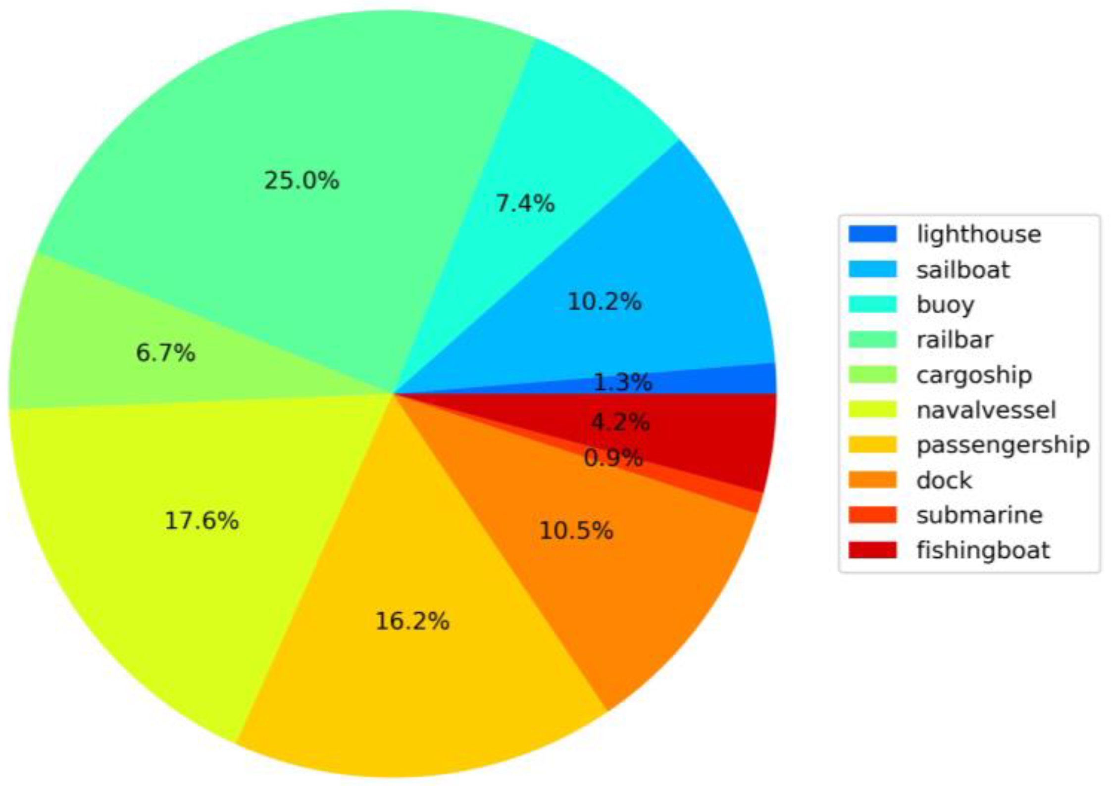
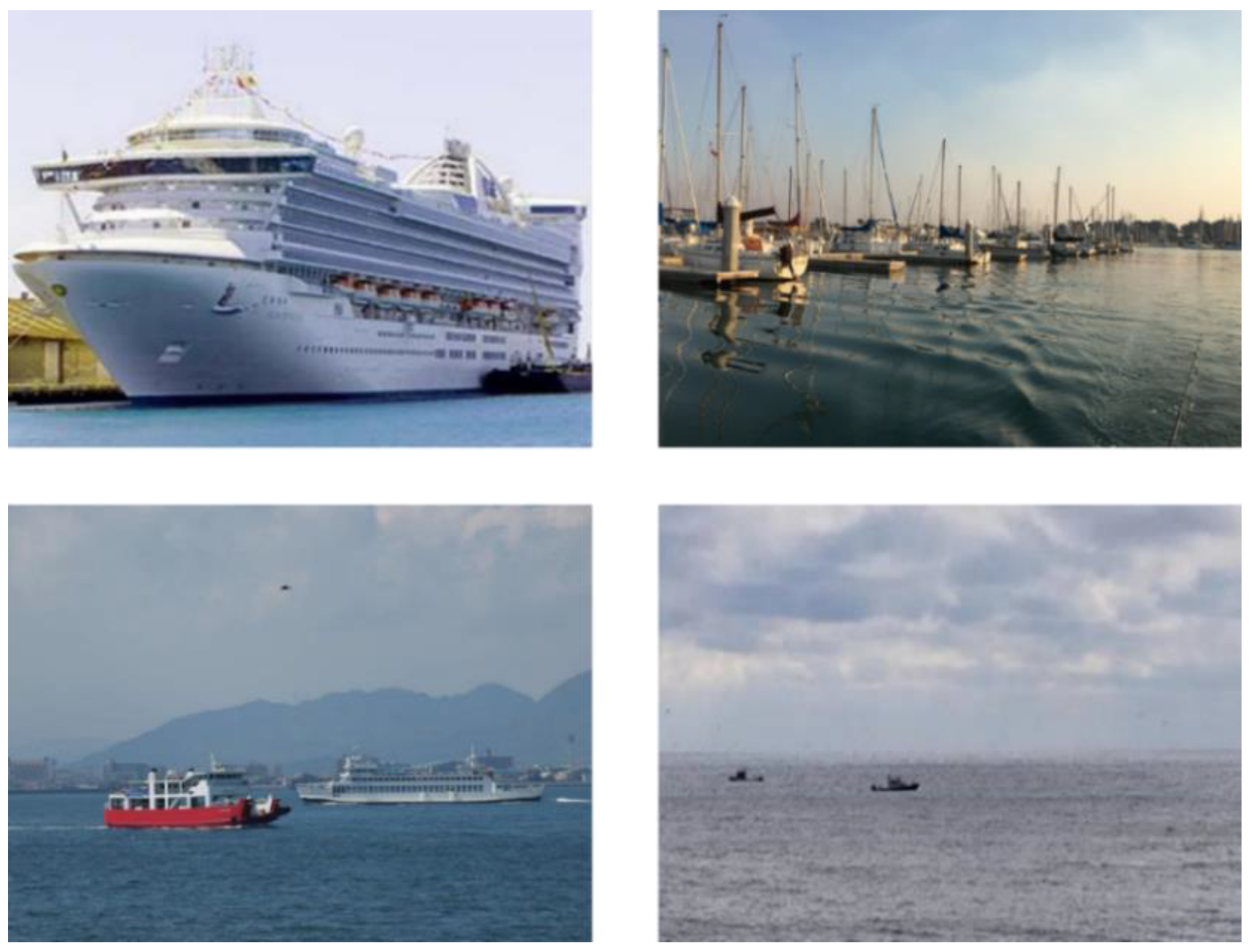
2.1. Description of the Maritime Target Dataset

A new dataset has been established that consists of typical targets in the river and sea regions well suited for the study and application of object recognition in marine engineering problems. The data came from the following sources: photographs taken at the harbors, pictures taken by the unmanned surface vehicle, and images collected from the websites. After the collection of the dataset, the images were annotated manually in the YOLO format. The dataset contains a total of more than seven thousand real images composed of ten classes of maritime objects, including ships (passenger ships, sailboats, cargo ships, etc.) and devices and structures (rail bars, lighthouses, docks, etc.), with an approximate ratio of 7:1:2 for the training, validation, and test sets. Figure 1 shows the distribution of targets from each of the ten categories in this dataset for training and validation, and image samples are displayed in Figure 2. Input images of the dataset vary in resolution and size. Images with medium to large targets accounting for the majority of the data are considered as one of the features of this dataset.

Challenges of this dataset come from the following aspects. Firstly, target classes are unevenly distributed, with certain types accounting for very small percentages among all the categories. In addition, the dataset contains a small portion of what can be referred to as hard examples, which include objects that appear small or tiny and images blurred due to harsh weather conditions. Moreover, new categories such as dock and rail bar are incorporated in the data, and in particular, docks have rather different characteristics compared to common categories such as boats or ships. These factors can potentially bring barriers to the learning of the model, which makes it necessary to put forward well-designed or specialized algorithms for the recognition of maritime objects.

2.2. Selected Model and Improvements

The basic model selected for our detection task contains several changes based on the yolov5m6 [12] baseline model. Here ‘6′ denotes ‘P6′, which means an extra P6 object output layer is added in the yolov5-P6 models for the detection of larger objects. Synchronized batch normalization [26], multi-scale training, and cosine learning rate are applied to assist the process of training, and the merge-NMS (non-maximum suppression) algorithm is used to remove redundant boxes for the same target during inference. The Mosaic method is used as an efficient technique that randomly selects three additional images for each image sample with cropping and scaling and combines them into one image, which will then be input into the network. The technique of label smoothing can be introduced in the computation of cross-entropy loss to prevent the model from being overconfident in classifying different types of objects which can be a source of over-fitting [27]. Mixup is an augmentation method that stacks two images into one with different weights. We will incorporate the methods of label smoothing and mixup optionally in some of our tests and analyze their effectiveness.

Considering the characteristics of our dataset, a main concern of this study is the problem of an unbalanced distribution of classes and hard examples in our dataset, which makes training difficult for certain objects. As an attempt to tackle this problem, the data pre-processing algorithms are strengthened by including combinations of auxiliary augmentation methods, which can enrich the features of each class to be learned by the model and improve the generalizability of the network. Another adjustment is to modify the loss function based on the idea of guiding the training process by taking the quality of samples into account. These practices will be described in more detail in the rest of this section.

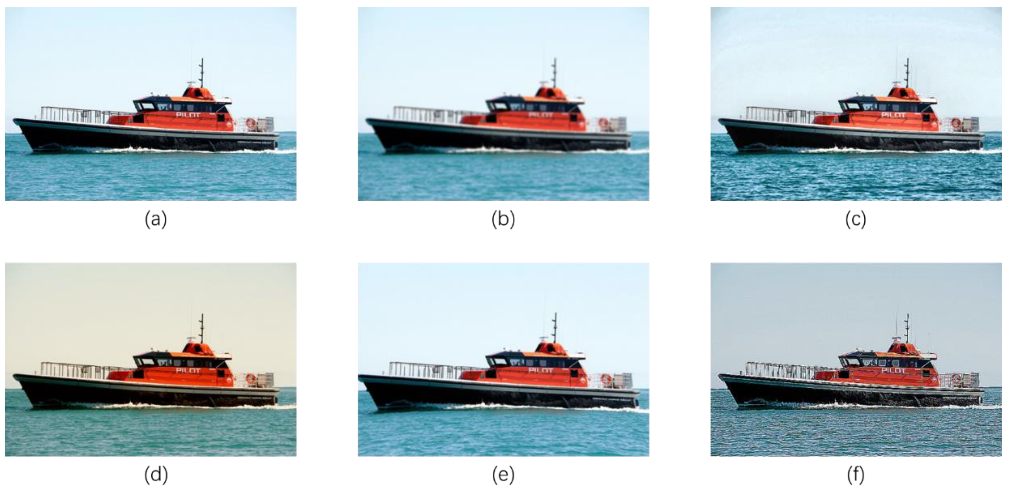
2.3. Tricks of Data Augmentation

To enhance the generalization ability of the model and reduce overfitting, in addition to the commonly used techniques such as Mosaic and mixup, multiple augmentation algorithms are introduced from the Albumentations package [28] into the algorithm as a part of the pre-processing procedure during training. We divide these augmentation methods into several groups according to their types and similarities with one another for the convenience of comparative study and result analysis. The sets of augmentation algorithms are listed as follows: Group A: random brightness contrast, random gamma, RGB shift, and CLAHE (associated with color transforms at the pixel level); Group B: either blur, median blur, or defocus (image blurring); Group C: shift scale rotate and optical distortion (transforms at the spatial level); Group D: grid distortion (another method of spatial transform); Group E: sharpen (which makes edges and profiles of objects clearer). Illustrations for several of these augmentation methods are provided in Figure 3.

It should be emphasized that the selections of the transform methods that are optimal or close to optimal are not obvious, and much effort is required to determine the combinations of methods that can achieve superior performance with the relevant data. The combinative impact of the selected groups among the whole set will be analyzed in the ablation studies.

2.4. Improvement in Loss Function

The bounding box regression loss function in the YOLOv5 algorithm reflects the Intersection over Union (IOU) between the predicted box and the ground-truth box, which should be optimized during the training process:

$$IoU=\frac{\left|A\cap B\right|}{\left|A\cup B\right|}$$

(1)

where $A$ and $B$ denote the ground-truth box and the predicted box, respectively. A basic and commonly used form of bounding box loss is the generalized IOU (GIOU) loss [23], but it tends to result in slow convergence and relatively low accuracy. In the particular cases where one of the boxes is contained in another, GIOU degrades to IOU, which makes the objective function less efficient. An improved formulation of the loss function is the complete IOU (CIOU) loss [24], defined as

$$L_{CIOU}=1-IOU+\frac{{\rho }^2}{c^2}+\alpha v$$

(2)

$$v=\frac{4}{{\pi }^2}{\left(\arctan \frac{w^{gt}}{h^{gt}}-\arctan \frac{w}{h}\right)}^2$$

(3)

$$\alpha =\frac{v}{1-IOU+v}$$

(4)

In the equations above, $\rho$ stands for the Euclidean distance between the central points of the predicted box B and the target box $B^{gt}$ ($b$ and $b^{gt}$), c is the diagonal length of the smallest enclosing box covering both boxes, and v measures the difference in the width-to-height ratio. Recently, Zhang et al. (2021) [25] proposed efficient IOU (EIOU), a modified form of loss function based on CIOU:

$$L_{EIOU}=1-IOU+\frac{{\rho }^2\left(b,b^{gt}\right)}{c^2}+\frac{{\rho }^2\left(w,w^{gt}\right)}{{\left(w^c\right)}^2}+\frac{{\rho }^2\left(h,h^{gt}\right)}{{\left(h^c\right)}^2}$$

(5)

where $w^c$ and $h^c$ denote the width and height of the smallest enclosing box covering B and $B^{gt}$. The EIOU loss directly takes into account the relative discrepancies of widths and heights instead of the width-to-height ratios. In this work, we take one further step in the modification of the loss function by revising EIOU into the following form:

$${\tilde{L}}_{EIOU}=L_{EIOU}{\left(IOU+\beta \right)}^{\gamma }$$

(6)

The parameters $\beta$ and $\gamma$ are set to be constants that can be tuned. The major aim of this modified formulation is to make the network focus more on the high-quality anchor boxes by placing more weights on these boxes relative to those with a lower IOU score. In other words, boxes that are more relevant to the targets have a greater influence on the bounding box loss function, thus enhancing convergence during the optimization process. $\beta$ and $\gamma$ serve to control the extent to which the effects of irrelevant frames are diminished by manipulating the shape of the coefficient. $\beta >0$ is required since the boxes with the IOU value of zero can be potential candidates for the localization of the target and are not negligible in the loss function. The weight becomes a concave function of IOU when $\gamma <1$, the hyperparameter range which proves favorable for our testing, in which case only the gradients of the anchor boxes with very small overlap ratio are significantly weakened. The revised loss function is relatively simple in its formulation and does not require additional treatment for the initialization of the optimization process as long as the parameters are set within an appropriate range.

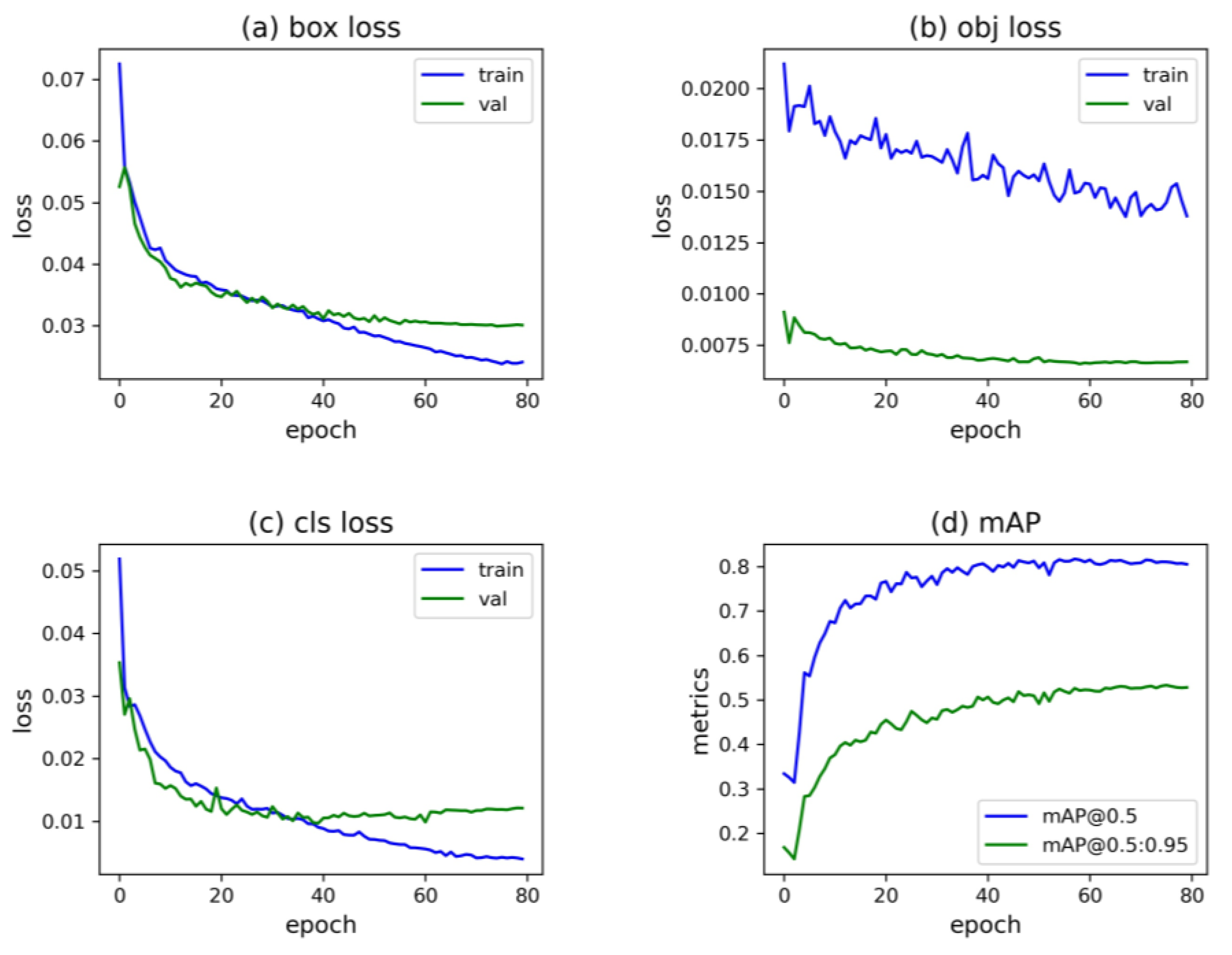
3. Results and Discussions

3.1. Setup of Experiments and Evaluation Metrics

In all of the tests, the model was trained for 80 epochs after loading the pre-trained weights from yolov5m6. The stochastic gradient descent (SGD) method was applied to optimize the loss function, with the initial learning rate set to 0.01. The configurations used for our tests were Tesla K80 GPUs with torch 1.7.1. Each model was trained with two GPUs. The results are mainly measured by the metric of mean average precision, $mAP=mAP@0.5:0.95$. Precision (Pr), recall (Re), and the F1 score will also be presented in several of the tests for reference. These metrics are formulated as follows:

$$Pr=\frac{TP}{FP+TP}$$

(7)

$$Re=\frac{TP}{FN+TP}$$

(8)

$$F1=\frac{2\times Pr\times Re}{Pr+Re}$$

(9)

$$mAP=\frac{1}{C}{{\displaystyle \sum }}_{i=1}^{C}A{P}_i$$

(10)

In the equations above, true positives (TP) stand for targets correctly recognized by the model. False positives (FP) stand for targets that are incorrectly detected. False negatives (FN) represent cases where targets are not detected. Average precision (AP) is the area under the precision–recall curve. Mean average precision (mAP) is the AP score averaged among all categories.

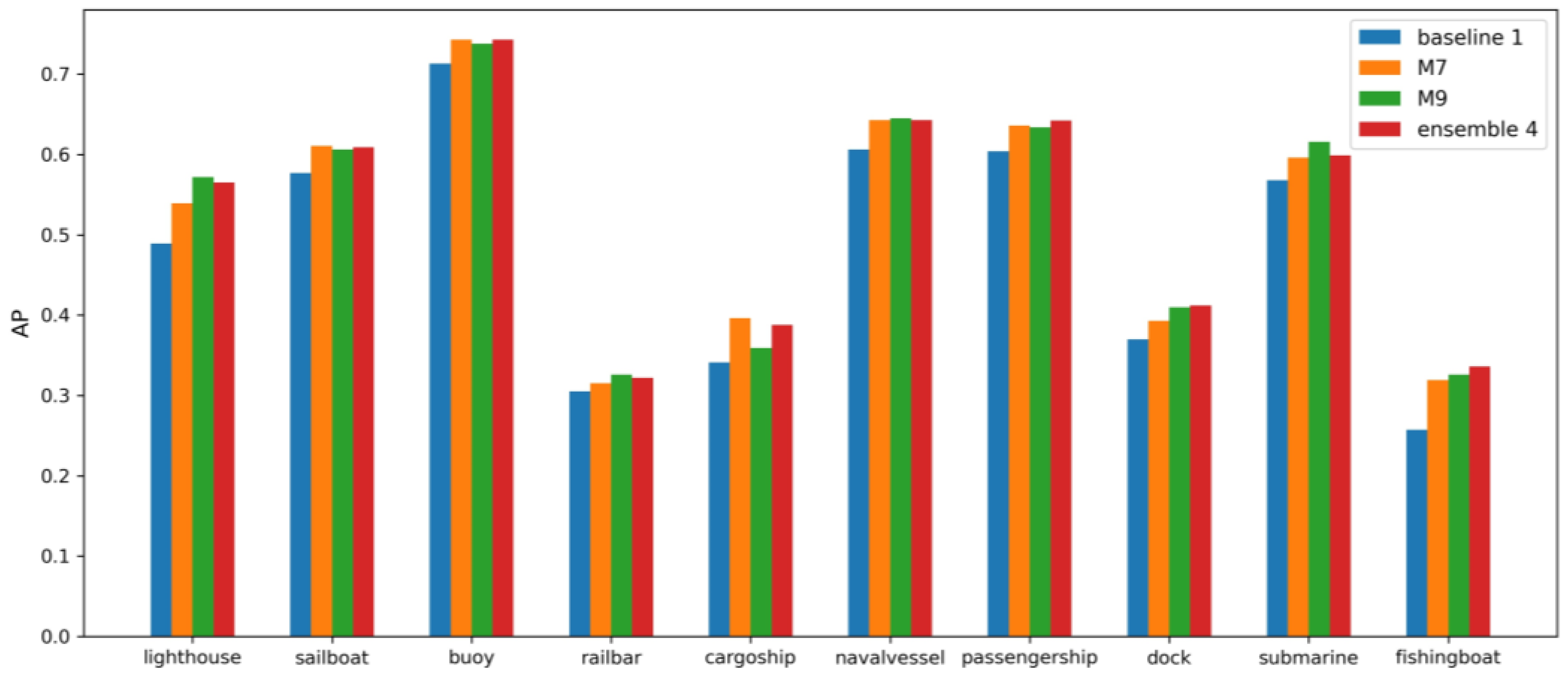
3.2. Results of the Baseline Models

As basic tests for the detector, we conducted experiments on the default baseline (the model with the default settings, which is referred to as Baseline 1) and the model with the selected settings described in Section 2.2 and test-time augmentation (which is referred to as Baseline 2). Both models were trained with the CIOU loss function and without the auxiliary augmentation packages.

Table 1. Test results for the baseline models.

Tests	Pr	Re	F1	mAP (%)
Baseline 1	0.835	0.766	0.799	48.3
Baseline 1 + TTA	0.849	0.76	0.802	49
Baseline 2	0.844	0.771	0.806	49.6

shows the mAP and the other scores evaluated on the test set using Baseline 1, the same baseline with test-time augmentation (TTA), and Baseline 2. The technique of TTA strengthens the inference performance with an increase of 0.7% in mAP. The advanced settings we applied improved the mAP score by another 0.6%. The F1 score grows steadily as more of the techniques are adopted. These results indicate that our settings are reasonable and constructive to the performance of the algorithm.

However, targets missed or misclassified by the baseline algorithm remain a tricky problem in the tests, which is partly attributed to the challenging data composed of the various categories. Strategies for enhancing the object detector will be introduced, which have the potential to alleviate this situation.

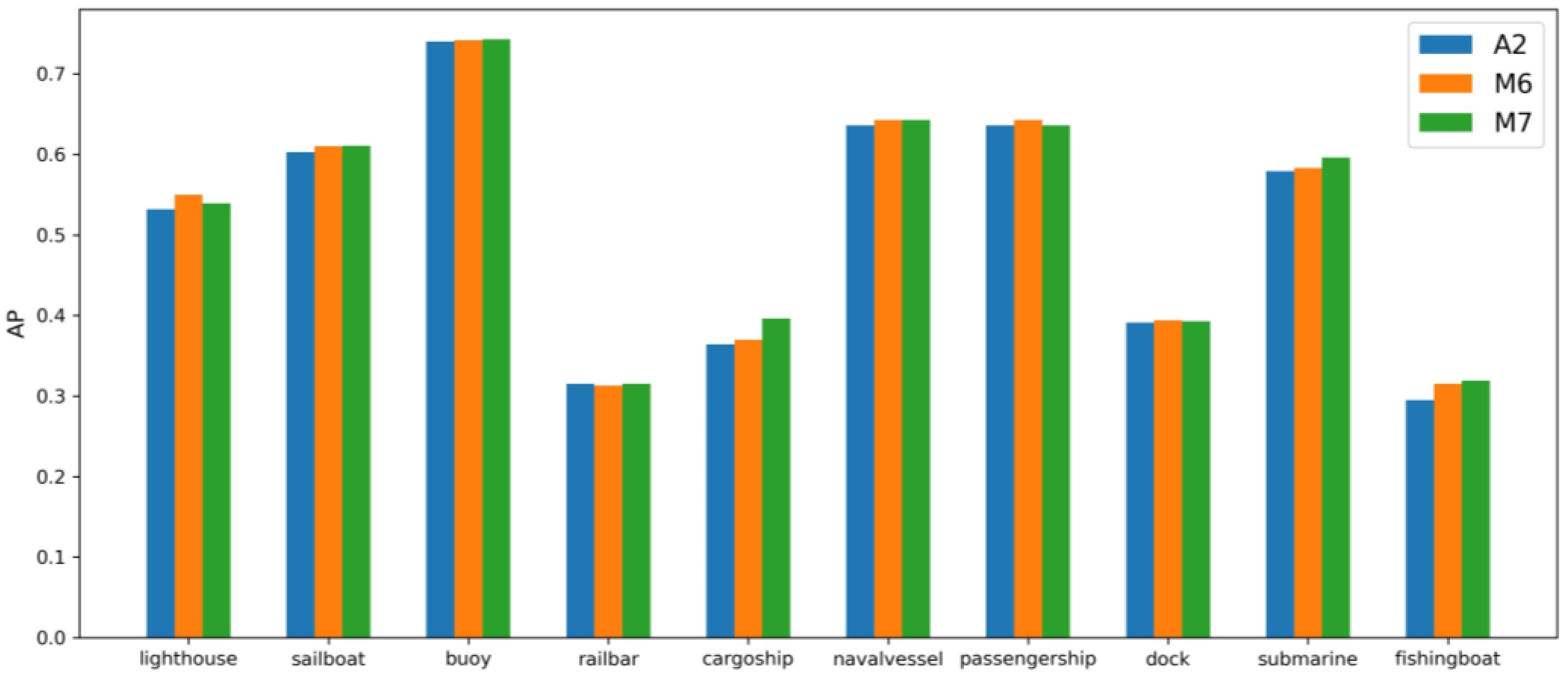
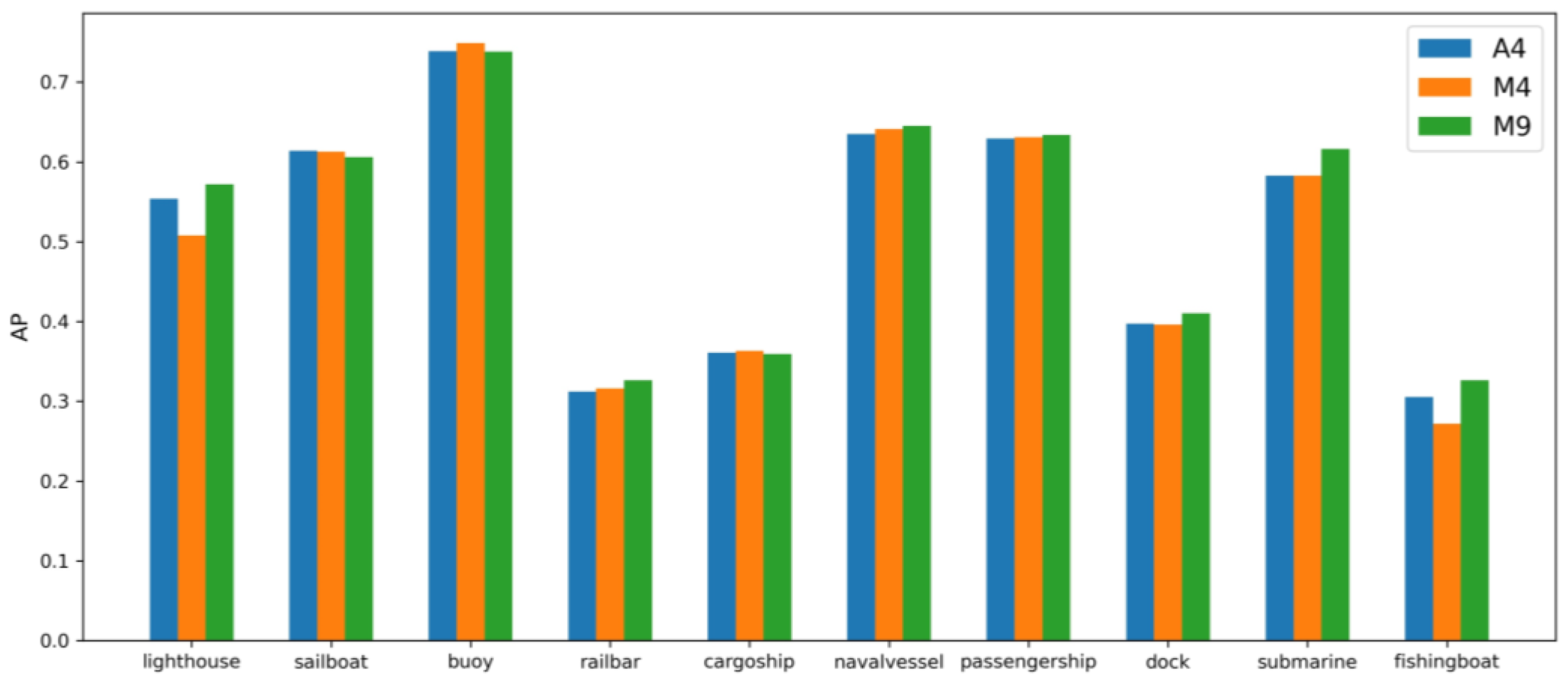
3.3. Ablation Tests with Data Augmentation

Here the focus of the tests is extended beyond the basic algorithms by studying the effects of the additional data augmentation techniques (Groups A to E in Section 2.3). Experiments were conducted by introducing multiple combinations of the transforms on the input data to Baseline 2 in order to reveal the effectiveness of the different groups. Based on our previous tests and observation of the results, we found that settings for the inference algorithm, such as those for NMS, also played a significant part in the average precision level, apart from the neural network and the pre-processing steps. Therefore, the different NMS settings Ⅰ and Ⅱ will be considered, where Ⅰ denotes the default setting of $thres=0.65$, and Ⅱ denotes $thres=0.4$. The results from the test set augmented with various sets of transforms are shown in

Table 2. Test results from the models augmented with different methods.

Test	Augmentation Groups	Setting	Pr	Re	mAP (%)
A1	A, B, C	Ⅰ	0.825	0.786	50.4
A2	A, B, C	Ⅱ	0.835	0.787	50.9
A3	D, E	Ⅰ	0.815	0.777	50.8
A4	D, E	Ⅱ	0.826	0.797	51.3
A5	C(H), D, E	Ⅰ	0.813	0.784	51
A6	C(H), D, E	Ⅱ	0.824	0.786	51.3
A7	A, B, C, D, E	Ⅰ	0.843	0.767	51
A8	A, B, C, D, E	Ⅱ	0.823	0.796	51.6

Note: the mark (H) stands for a higher probability for the particular group.

.

The combined augmentation sets that have been employed all lead to a fairly large boost in the average precision score. Tested with the default threshold value, the increase in mAP relative to Baseline 2 ranges from 0.8% to 1.4%. Switching the NMS setting from Ⅰ to Ⅱ gives an additional improvement in the mAP and F1 scores in each of the cases and raises both precision and recall in most scenarios. A lower IOU threshold in the NMS process tends to produce better results in these cases since most of the targets in our dataset are rather sparsely distributed, and this adjustment may eliminate more redundant boxes generated from the trained model and TTA. Therefore, results obtained with setting Ⅱ will be considered for the following discussion unless specified otherwise.

The augmentation Groups D and E prove to be a slightly more effective combination compared to the set of A, B, and C. Incorporating the distortion transforms of C into the set (D, E) gives no more increase in the average precision. This may result from the counteraction between the different sets. In other words, the compound impact of two or more augmentation techniques from the general perspective is not known in advance, which makes verification through experiments a simple and effective practice in order to reveal the effects. The complete set of A, B, C, D, and E achieves the best mAP of 51.6% among the cases that we have tested for the augmentation methods.

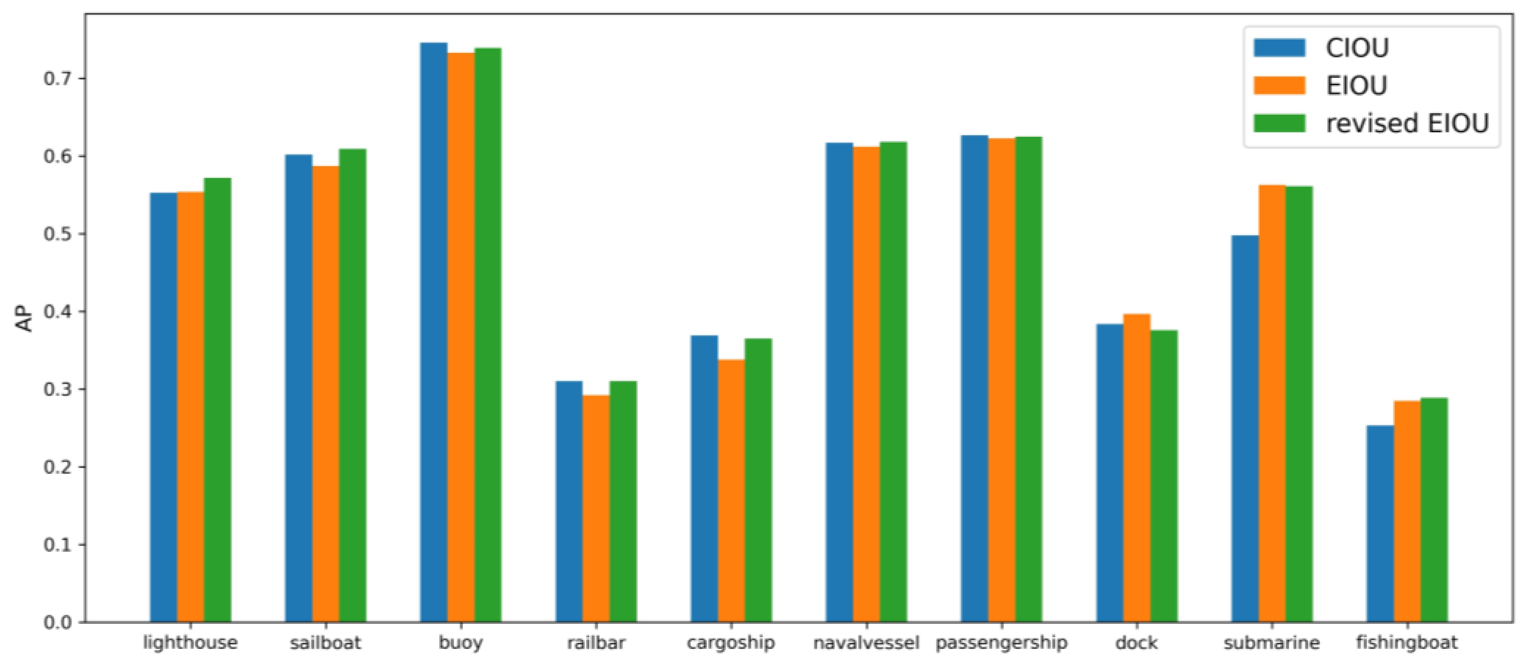
3.4. Ablation Tests with the Adapted Loss Function

To demonstrate the effects of the box loss function on the model performance, we compare results from the detectors with the CIOU loss, the EIOU loss, and the revised EIOU loss. It should be noted that the new formulation of the loss function has certain flexibility in the parameters $\gamma$ and $\beta$. Based on prior testing on a variety of cases, we set $\gamma =0.5$ and $\beta =0.1$ as the default parameters for the revised EIOU loss in the comparative studies. Results using $\beta =0.1$ and different values of $\gamma$ for Baseline Model 2 with the loss function altered to the adapted EIOU loss have been appended in

Table 3. Tests for the revised EIOU loss with varying $\gamma$ values.

$\mathbf{\gamma }$	0.3	0.4	0.5	0.6	0.7
mAP (%)	50.5	51.0	50.9	51.0	50.2

. Considering the reference result with the unaltered EIOU loss (

Table 4. Test results using different loss functions, augmentation sets, and other settings.

Test	Loss Function	Augmentation Groups	Additional Techniques	mAP (%)
M1	$L_{EIOU}$	$-$	Setting Ⅰ	49.8
M2	$L_{EIOU}$	$-$	$-$	50.1
M3	${\tilde{L}}_{EIOU}$	$-$	$-$	50.9
M4	${\tilde{L}}_{EIOU}$	D, E	$-$	50.7
M5	${\tilde{L}}_{EIOU}$	A, B, C, D, E	$-$	51.6
M6	${\tilde{L}}_{EIOU}$	A, B, C	$-$	51.6
M7	${\tilde{L}}_{EIOU}$	A, B, C	mixup, label smoothing	51.9
M8	${\tilde{L}}_{EIOU}$	A, B, C, D, E	mixup, label smoothing	51.4
M9	${\tilde{L}}_{EIOU}$	D, E	mixup, label smoothing	52.3

), the new formulation achieves considerable growth in mAP score when $\gamma$ is around $0.4 ~ 0.6$, which indicates that improvements provided by the proposed algorithm are stable and sufficiently consistent over the hyperparameter range. $\gamma =0.5$ is in the middle of this range and has been shown to be robust in the model performance among various cases.

The test cases and results with EIOU loss or revised EIOU loss are shown in Table 4, where the threshold setting Ⅱ has been applied as the default setting. Figure 4 shows the learning curves for the model trained with the adapted loss function (Test M3). The training losses generally drop steadily during the entire process, while losses for validation all reach the minimum values prior to the last epoch. Similarly, the mAP curves obtain their peaks before going down near the end of the training. These trends verify that settings, including the total number of epochs and our proposed form of the loss function, are appropriate for the experiments.

The original EIOU loss produces a mAP score similar to the CIOU loss (Baseline 2), with a difference of merely 0.2% between the two different forms, while selecting the adapted form with NMS setting Ⅱ leads to an overall improvement of 1.3% compared to Baseline Model 2. This trend is maintained for the tests augmented with the first three groups of image transformation methods, where the mAP score reaches 51.6%, growing by 0.7% compared to the model using the default CIOU loss. The situation changes when sets D and E (representing the local distortions and sharpening of the images) are incorporated in the pre-processing steps. These two no longer contribute to further improvements in average precision, seemingly in contrast to the conclusion we have drawn previously that the set of D and E alone is more efficient (than the combination of A, B, and C) in enhancing the predictive results. It is assumed that this may partly be related to the features of augmentation methods in these sets. Transforms in this combination either enrich the dataset or make targets more recognizable, while the new loss function serves to reset the weights for the boxes and diminish the influence of the ones with poor quality. Judging by the statistics, these two methods do not work sufficiently well when combined together.

For the testing of the complete sets of methods, we incorporate the optional techniques (mixup and label smoothing) in the compound models with the selected augmentation sets. The results are shown as Tests M7 to M9, where the model with augmentation (D, E) achieves the highest mAP among the individual models that have been discussed. From the perspective of combinations of augmentation methods, this result is in contrast to the trend in the previous tests without the optional techniques. Scores for the model augmented with the sets (A, B, C) and the one with the sets (D, E) are both improved when the two techniques are employed, while this trend no longer applies to the case with all the augmentation sets (A, B, C, D, E) selected. Again, this observation indicates that the composite method consisting of a variety of techniques has complicated effects, where the contribution of each individual ingredient may seem to be suppressed by different degrees when combined with one another and may reach a certain bottleneck where simple addition of techniques can no longer raise the performance of the detector. To further verify the effects of the modified EIOU loss, we have repeated the tests with the different augmentation sets (M4 to M9) using the original EIOU loss function. The revised EIOU function holds an advantage over EIOU in the test accuracy for most of the cases, with an average mAP improvement of 0.9% for the six tests and a maximum improvement of more than 2%. These statistics are a good indication of the superiority of the proposed loss function when combined with the augmentation algorithms and other techniques.

The AP scores for each type of target are illustrated in Figure 5, Figure 6 and Figure 7 for a closer analysis of the different improvements. Compared to the CIOU loss, noticeable increases in AP ($\ge 1\%$) produced by revised EIOU loss occur for the three categories that account for the smallest percentages in the training and validation data. It indicates that the new loss function is most constructive in raising the inference accuracies of the targets which appear least frequently and is capable of ameliorating the problem of the uneven data distribution to some extent. With the augmentation sets A, B, and C selected, the modified loss function provides remarkable AP improvements for lighthouses (+1.8%) and fishing boats (+2%) and moderate improvements for all the other categories except rail bar, showing a tendency generally similar to the previous case with the revised loss alone. The situation changes when the model is augmented with Groups D and E, where the test accuracy drops mostly due to the two categories (lighthouse and fishing boat). Prediction is further enhanced only when the optional techniques of mixup and label smoothing are employed. This observation may be attributed to the following factors: (1) There are only a total of two transform methods in the set (D, E). (2) This combination is associated with strong spatial distortions, which make the performance of the detector less stable when functioning along with other methods. The optional techniques, in general, contribute positively to the classes with very few objects ($\le 5\%$) and may lead to a noticeable increase in AP for certain categories with low AP scores, e.g., cargo ship for M7, rail bar, and dock for M9, which are either easily confused with other classes or hard to detect and localize accurately.

As a possible solution to the problem mentioned above, the approach of using a model ensemble can be employed to take advantage of the superiorities of models with different characteristics. The ensemble model comprising the best individual models (M7 and M9) has been constructed as our refined method. We also tested the performance of other ensemble models constructed with the existing frameworks shown in Table 2 and Table 4. The relevant models, along with the scores, are demonstrated in

Table 5. Test results using ensemble models.

Test	Ensemble Models	mAP (%)
Ensemble 1	(A8, M3)	51.8
Ensemble 2	(M4, M6)	51.5
Ensemble 3	(M5, M7)	52.2
Ensemble 4 (proposed method)	(M7, M9)	52.6

. To be more specific, Ensemble 1 combines the effects of all the augmentation methods (with the CIOU loss) and the revised EIOU loss function. In test cases for Ensemble 2 and Ensemble 4, integration of the model using the augmentation sets (A, B, C) and the one using (D, E) is evaluated, while in Ensemble 3, the individual models differ in the settings for augmentation and additional techniques. The accuracy of the ensemble model surpasses the individual model that has a higher score in most of these cases, even when the discrepancy between the individual models is relatively large. Our proposed method, Ensemble Model 4, which benefits from the improved loss function and combines the superior strategies for data augmentation algorithms and other techniques, achieves the highest mAP of 52.6% (+4.3% compared to Baseline 1), which is higher than that of the best individual model.

In order to perform a further analysis of the test accuracies of the models, we plotted a bar graph of the AP scores for each category produced with the baseline model (Baseline 1) and our methods (M7, M9, and Ensemble 4) on the test set in Figure 8. It can be seen when comparing the two single models with the highest accuracies to the baseline model that the accuracy for each category is enhanced in both of these two test cases. The AP value of the ensemble model lies either above the higher score or between the AP scores of the two relevant models. Boosts in the AP scores resulting from the ensemble model compared with the baseline are relatively stable among the categories, lying between +3% and +5% for most of the classes, except for fishing boat (+7.9%), lighthouse (+7.6%), and rail bar (+1.7%). In other words, the improvements and tricks adopted in this model have remarkable effects on the recognition of fishing boats and lighthouses and are shown to be least effective in detecting rail bars, the latter of which is one of the challenging problems of this dataset.

Typical results generated by Ensemble Model 4 are presented in Figure 9 (2nd column). Comparison with Baseline 2 (1st column) indicates that the current model with the synthesized techniques overcomes many of the shortcomings of the results predicted by the baseline model via reducing incorrect annotations for the target category, removing some false detections of irrelevant or unrecognizable objects, and identifying targets missed by the previous model in certain circumstances, etc. However, the new algorithm might perform poorer when recognizing small objects. This can possibly be attributed to the characteristics of the revised loss function, which may suppress the learning of small objects since the anchor boxes are less likely to have large overlaps with these targets. Both models have limitations in the recognition of complex targets or those from complicated or blurred backgrounds, e.g., the misclassification of the background as a dock in Figure 9(a2,b2).

4. Conclusions

This work carried out a study on the application of the improved YOLOv5 model to object detection tasks with the dataset containing targets of typical categories in the sea and river environments. Multiple sets of image transformation techniques were used to augment the input data. The effectiveness of several syntheses of these sets and their impact on the generalization ability of the detector were discussed and analyzed. In addition, a modification was made to the EIOU loss function, which serves to enhance the relative significance of the high-quality anchor boxes. Comparing the cases of different combinations of the loss function, augmentation algorithms, and model settings, it can be concluded that the revised loss function, in general, leads to a further boost in the inference ability and that the proposed method with the superior strategy for the combined algorithms manages to compensate for several deficiencies of the previous model when evaluated on our data, in spite of the challenges such as unbalanced distribution of the categories and hard samples posed by the dataset. Restrictions of the current model exist in the recognition of targets from complex backgrounds. It is believed that the effects of the augmentation methods and the revised loss function are generalizable to a wider range of applications, which will be investigated in future work.

References

1. Er, M.J.; Zhang, Y.; Chen, J.; Gao, W. Ship detection with deep learning: A survey. Artif. Intell. Rev. 2023, 2023, 1–41. [Google Scholar] [CrossRef]
2. He, Y.; Zhu, C.; Wang, J.; Savvides, M.; Zhang, X. Bounding Box Regression With Uncertainty for Accurate Object Detection. In Proceedings of the IEEE/CVF Conference on Computer Vision and Pattern Recognition, Salt Lake City, UT, USA, 18–23 June 2018; pp. 2883–2892. [Google Scholar]
3. Benjumea, A.; Teeti, I.; Cuzzolin, F.; Bradley, A. YOLO-Z: Improving small object detection in YOLOv5 for autonomous vehicles. arXiv 2021, arXiv:2112.11798. [Google Scholar]
4. Zhang, H.; Chang, H.; Ma, B.; Wang, N.; Chen, X. Dynamic R-CNN: Towards High Quality Object Detection via Dynamic Training. arXiv 2020, arXiv:2004.06002. [Google Scholar]
5. Girshick, R.B.; Donahue, J.; Darrell, T.; Malik, J. Rich Feature Hierarchies for Accurate Object Detection and Semantic Segmentation. In Proceedings of the IEEE Conference on Computer Vision and Pattern Recognition, Portland, OR, USA, 23–28 June 2013; pp. 580–587. [Google Scholar]
6. Girshick, R.B. Fast R-CNN. In Proceedings of the IEEE International Conference on Computer Vision, Santiago, Chile, 7–13 December 2015; pp. 1440–1448. [Google Scholar]
7. Ren, S.; He, K.; Girshick, R.B.; Sun, J. Faster R-CNN: Towards Real-Time Object Detection with Region Proposal Networks. IEEE Trans. Pattern Anal. Mach. Intell. 2015, 39, 1137–1149. [Google Scholar] [CrossRef] [PubMed] [Green Version]
8. Dai, J.; Li, Y.; He, K.; Sun, J. R-FCN: Object Detection via Region-based Fully Convolutional Networks. arXiv 2016, arXiv:1605.06409. [Google Scholar]
9. Cai, Z.; Vasconcelos, N. Cascade R-CNN: Delving Into High Quality Object Detection. In Proceedings of the IEEE/CVF Conference on Computer Vision and Pattern Recognition, Honolulu, HI, USA, 21–26 July 2017; pp. 6154–6162. [Google Scholar]
10. He, K.; Gkioxari, G.; Dollár, P.; Girshick, R.B. Mask R-CNN. IEEE Trans. Pattern Anal. Mach. Intell. 2017, 42, 386–397. [Google Scholar] [CrossRef] [PubMed]
11. Redmon, J.; Divvala, S.K.; Girshick, R.B.; Farhadi, A. You Only Look Once: Unified, Real-Time Object Detection. In Proceedings of the IEEE Conference on Computer Vision and Pattern Recognition, Boston, MA, USA, 7–12 June 2015; pp. 779–788. [Google Scholar]
12. Jocher, G. Yolov5. 2020. Available online: https://github.com/ultralytics/yolov5 (accessed on 1 September 2022).
13. Liu, W.; Anguelov, D.; Erhan, D.; Szegedy, C.; Reed, S.E.; Fu, C.-Y.; Berg, A.C. SSD: Single Shot MultiBox Detector. In Proceedings of the European Conference on Computer Vision, Amsterdam, The Netherlands, 11–14 October 2016. [Google Scholar]
14. Lin, T.-Y.; Goyal, P.; Girshick, R.B.; He, K.; Dollár, P. Focal Loss for Dense Object Detection. IEEE Trans. Pattern Anal. Mach. Intell. 2017, 42, 318–327. [Google Scholar] [CrossRef] [PubMed] [Green Version]
15. Everingham, M.; Gool, L.V.; Williams, C.K.I.; Winn, J.M.; Zisserman, A. The Pascal Visual Object Classes (VOC) Challenge. Int. J. Comput. Vis. 2010, 88, 303–338. [Google Scholar] [CrossRef] [Green Version]
16. Wang, Y.; Bashir, S.M.A.; Khan, M.; Ullah, Q.; Wang, R.; Song, Y.; Guo, Z.; Niu, Y. Remote Sensing Image Super-resolution and Object Detection: Benchmark and State of the Art. Expert. Syst. Appl. 2021, 197, 116793. [Google Scholar] [CrossRef]
17. Lin, T.-Y.; Dollár, P.; Girshick, R.B.; He, K.; Hariharan, B.; Belongie, S.J. Feature Pyramid Networks for Object Detection. In Proceedings of the IEEE Conference on Computer Vision and Pattern Recognition, Las Vegas, NV, USA, 27–30 June 2016; pp. 936–944. [Google Scholar]
18. Sun, X.M.; Zhang, Y.J.; Wang, H.H.; Du, Y. Research on ship detection of optical remote sensing image based on Yolo V5. J. Phys. Conf. Ser. 2022, 2215, 012027. [Google Scholar] [CrossRef]
19. Zhang, X.; Yan, M.; Zhu, D.; Guan, Y. Marine ship detection and classification based on YOLOv5 model. J. Phys. Conf. Ser. 2022, 2181, 012025. [Google Scholar] [CrossRef]
20. Pang, L.; Li, B.; Zhang, F.; Meng, X.; Zhang, L. A Lightweight YOLOv5-MNE Algorithm for SAR Ship Detection. Sensors 2022, 22, 7088. [Google Scholar] [CrossRef] [PubMed]
21. Lei, F.; Tang, F.; Li, S. Underwater Target Detection Algorithm Based on Improved YOLOv5. J. Mar. Sci. Eng. 2022, 10, 310. [Google Scholar] [CrossRef]
22. Liu, Z.; Zhuang, Y.; Jia, P.; Wu, C.; Xu, H.; Liu, Z. A Novel Underwater Image Enhancement Algorithm and an Improved Underwater Biological Detection Pipeline. J. Mar. Sci. Eng. 2022, 10, 1204. [Google Scholar] [CrossRef]
23. Rezatofighi, S.H.; Tsoi, N.; Gwak, J.; Sadeghian, A.; Reid, I.D.; Savarese, S. Generalized Intersection Over Union: A Metric and a Loss for Bounding Box Regression. In Proceedings of the IEEE/CVF Conference on Computer Vision and Pattern Recognition, Long Beach, CA, USA, 15–20 June 2019; pp. 658–666. [Google Scholar]
24. Zheng, Z.; Wang, P.; Liu, W.; Li, J.; Ye, R.; Ren, D. Distance-IoU Loss: Faster and Better Learning for Bounding Box Regression. In Proceedings of the AAAI Conference on Artificial Intelligence, New York, NY, USA, 7–12 February 2020. [Google Scholar]
25. Zhang, Y.-F.; Ren, W.; Zhang, Z.; Jia, Z.; Wang, L.; Tan, T. Focal and Efficient IOU Loss for Accurate Bounding Box Regression. Neurocomputing 2021, 506, 146–157. [Google Scholar] [CrossRef]
26. Peng, C.; Xiao, T.; Li, Z.; Jiang, Y.; Zhang, X.; Jia, K.; Yu, G.; Sun, J. MegDet: A Large Mini-Batch Object Detector. In Proceedings of the IEEE/CVF Conference on Computer Vision and Pattern Recognition, Honolulu, HI, USA, 21–26 July 2017; pp. 6181–6189. [Google Scholar]
27. Zhang, Z.; He, T.; Zhang, H.; Zhang, Z.; Xie, J.; Li, M. Bag of Freebies for Training Object Detection Neural Networks. arXiv 2019, arXiv:1902.04103. [Google Scholar]
28. Buslaev, A.V.; Parinov, A.; Khvedchenya, E.; Iglovikov, V.I.; Kalinin, A.A. Albumentations: Fast and flexible image augmentations. arXiv 2018, arXiv:1809.06839. [Google Scholar] [CrossRef] [Green Version]
Figure 1. Pie chart of data distribution of the targets from the ten categories in the training and validation sets.
Applsci 13 07695 g001
Figure 2. Image samples from the training set. These samples differ in their resolutions and have been rescaled to the same size here for convenient demonstration.
Applsci 13 07695 g002
Figure 3. Sample images processed by the data augmentation algorithms introduced in Section 2.3: (a) original; (b) defocus; (c) CLAHE; (d) RGB shift; (e) optical distortion; (f) sharpen. These results have been generated in a separate experiment for illustration purposes and may not reflect the situation in the training process of the model.
Applsci 13 07695 g003
Figure 4. Curves of the loss functions for the training and validation sets and the metrics during training using the revised EIOU loss function (model M3): (a) box loss; (b) confidence loss; (c) classification loss; (d) mAP.
Applsci 13 07695 g004
Figure 5. The average precision (AP) scores of the ten categories for the models with CIOU loss (Baseline 2), EIOU loss, and the revised EIOU loss. Results are obtained using NMS setting Ⅰ.
Applsci 13 07695 g005
Figure 6. The average precision (AP) scores of the ten categories for Models A2 (augmentation A, B, C), M6 (A2 + revised EIOU), and M7 (A2 + revised EIOU + additional techniques).
Applsci 13 07695 g006
Figure 7. The average precision (AP) scores of the ten categories for Models A4 (augmentation D, E), M4 (A4 + revised EIOU), and M9 (A4 + revised EIOU + additional techniques).
Applsci 13 07695 g007
Figure 8. The average precision (AP) scores of the ten categories for the Baseline 1, M7, M9, and Ensemble 4 models.
Applsci 13 07695 g008
Figure 9. Image samples with the annotated objects generated with Baseline Model 2 (subplots (a1a3)) and Ensemble Model 4 (b1b3).
Applsci 13 07695 g009