Multi-Objective Optimization of a Two-Stage Helical Gearbox Using Taguchi Method and Grey Relational Analysis

Abstract

This paper presents a novel approach to solve the multi-objective optimization problem designing a two-stage helical gearbox by applying the Taguchi method and the grey relation analysis (GRA). The objective of the study is to identify the optimal main design factors that maximize the gearbox efficiency and minimize the gearbox mass. To achieve that, five main design factors. including the coefficients of wheel face width (CWFW) of the first and the second stages, the allowable contact stresses (ACS) of the first and the second stages, and the gear ratio of the first stage were chosen. Additionally, two single objectives, including the maximum gearbox efficiency and minimum gearbox mass, were analyzed. In addition, the multi-objective optimization problem is solved through two phases: Phase 1 solves the single-objective optimization problem in order to close the gap between variable levels, and phase 2 solves the multi-objective optimization problem to determine the optimal main design factors. From the results of the study, optimum values of five main design parameters for designing a two-stage helical gearbox were first introduced.

1. Introduction

Optimizing gearboxes is a critical aspect of mechanical engineering as it has a direct impact on their efficiency, durability, and reliability, as well as the performance of other machinery and equipment. Multi-objective optimization of gearboxes involves simultaneously optimizing various performance parameters, such as load-carrying capacity, noise, mass, size, and efficiency, making it a complex and challenging task. To address these challenges, various optimization techniques have been developed in recent years. Helical gearboxes, one of many gearbox types, are widely used in industrial applications due to their superior load-carrying capacity, smooth operation [1], simple structure, and low cost. However, designing a helical gearbox involves numerous design parameters, making it difficult to optimize for multiple objectives.

Numerous studies on the optimal design of helical gearboxes have been conducted thus far. This research looked into both single-objective and multi-objective optimization problems. Many authors are also interested in the single-objective optimization problem. I. Römhild and H. Linke [2] presented formulas for calculating gear ratios for two-, three-, and four-stage helical gearboxes in order to obtain the smallest gear mass. Milou et al. [3] presented a practical approach for reducing the mass of a two-stage helical gearbox in their paper. The method entailed analyzing data from gearbox manufacturers. Their findings suggested a center distance ratio (aw₂/aw₁) between the second and first stages in the range of 1.4 to 1.6 to achieve the minimum mass. Once the optimal center distance ratio has been determined, the corresponding partial gear ratios are obtained using a lookup table. Various objective functions are utilized to solve the single-objective optimization problem of determining the optimal gear ratio of helical gearboxes. These objective functions include minimizing gearbox length [4,5,6,7], minimizing gearbox cross section area [6,8,9,10], minimizing gearbox mass [6,11], minimizing gearbox volume [12], and minimizing gearbox cost [13,14,15,16]. All of these studies share a common feature in that only one design parameter, the partial gear ratio, is defined in the form of an explicit model.

The multi-objective optimization problem for designing helical gearboxes has also been of interest to researchers. M. Patil et al. [1] conducted a study in which a two-stage helical gearbox was subjected to multi-objective optimization with a broad range of constraints using a specially formulated discrete version of non-dominated sorting genetical algorithm II (NSGA-II). The study formulated two objective functions, namely the minimum gearbox volume and minimum total gearbox power loss. Moreover, the study considered constraints, such as bending stress, pitting stress, and tribological factors. Wu, Y.-R. and V.-T. Tran [17] introduced a new microgeometry modification for helical gear pairs, leading to substantial enhancements in performance with regards to noise and vibration. In their research, C. Gologlu and M. Zeyveli [18] utilized a genetic algorithm (GA) to optimize the volume of a two-stage helical gearbox. To handle the design constraints, such as bending stress, contact stress, number of teeth on pinion and gear, module, and face width of gear, the objective function was subject to static and dynamic penalty functions. The results from the GA were compared to those of a deterministic design procedure, with the GA being found to be the superior method. D. F. Thompson and colleagues [19] presented a generalized optimization technique for reducing the volume of two-stage and three-stage helical gearboxes, while considering tradeoffs with surface fatigue life. In their study, Edmund S. Maputi and Rajesh Arora [20] explored multi-objective optimization by simultaneously considering three objectives: volume, power output, and center-distance. They employed the NSGA-II evolutionary algorithm to generate Pareto frontiers in their research. From the results of the study, insights for the design of compact gearboxes can be gained. The NSGA-II method was also applied by C. Sanghvi et al. [21] to solve the multi-objective optimization problem of a two-stage helical gearbox for minimum volume and maximum load. The results of the multi-objective optimization of the tooth surface in helical gears using the response surface method were presented by Park C.I. [22].

The best or optimal level of the selected criterion is determined by single-objective optimization, which is an absolute optimization. A multi-objective optimization problem is one with two or more simple goals (or criteria). As a result, the solution to the multi-objective optimization problem cannot best satisfy all criteria simultaneously. For instance, it is not possible to meet both the efficiency and cost requirements of the gearbox. In simple terms, determining a solution to a problem that is both “white” and “black” is impossible; only a “gray” solution can be determined. The gray solution is the one that falls between the best and worst solutions, or between “white” and “black” in the multi-objective optimization problem. As a result, it is known as optimization based on gray relation analysis. The original Taguchi method is used to solve the single-objective problem, and the Taguchi method and gray relation analysis are required to solve the multi-objective optimization problem.

While numerous studies have focused on multi-objective optimization for helical gearboxes, the identification of optimal main design factors for such gearboxes has not received adequate attention. Furthermore, previous research on multi-objective optimization for helical gearboxes has not demonstrated the relationship between optimal input factors and total gearbox ratio. This is a critical issue to consider when designing a new gearbox. In this paper, we present a multi-objective optimization study for a two-stage helical gearbox, considering two single objectives: minimizing gearbox mass and maximizing gearbox efficiency. The proposal of five optimal main design factors for the two-stage helical gearbox is the most significant result of this research. These variables include the CWFW for both stages, the ACS for both stages, and the first stage’s gear ratio. Furthermore, by combining the Taguchi method and the GRA in a two-stage process not previously described, we present a novel approach to addressing the multi-objective optimization problem in gearbox design. Additionally, a link between optimal input factors and the total gearbox ratio was proposed.

2. Optimization Problem

2.1. Gearbox Mass Calculation

The mass of the gearbox $m_{gb}$ can be found by the following equation:

$$m_{gb}=m_g+m_s+m_{gh}+m_b$$

(1)

where $m_g$, $m_{gh}$, $m_b$, and $m_s$ designate the mass of the gears, the shafts, the bearings, and the gearbox housing, respectively. The component mass will be specifically calculated below:

2.1.1. Gearbox Housing Mass Calculation

The gearbox housing mass ($m_{gh}$) can be found by:

$$m_{gh}={\rho }_{gh}·V_{gh}$$

(2)

in which ${\rho }_{gh}$ is the weight density of gearbox housing materials referred; as the material of the gearbox housing is gray cast iron (the most common material for the gearbox housing), ${\rho }_{gh}=7300 \left(\mathrm{k}\mathrm{g}/{\mathrm{m}}^3\right)$; $V_{gh}$ is the gearbox housing volume (m³), which is determined by the following equation (see Figure 1):

Figure 1. Calculated schema.

Figure 1. Calculated schema.

$$V_{gh}=2·V_A+2·V_B+2·V_C$$

(3)

where $V_A$, $V_B$, and $V_C$ are the volumes of side A, B, and C (m³), respectively.

$$V_A=L·H·S_G$$

(4)

$$V_B=L·B_1·1.5·S_G$$

(5)

$$V_C=B_2·H·S_G=\left(B_1-2·S_G\right)·H·S_G$$

(6)

Substituting Equations (4) to (6) into (3) obtains:

$$V_{gh}=2·L·H.S_G+3·L·B_1·S_G+2·\left(B_1-2·S_G\right)·H·S_G$$

(7)

In the above equations, L, H, B₁, and SG can be calculated by [2]:

$$L=(d_{w11}+d_{w21}/2+d_{w12}/2+d_{w22}/2+22.5)/0.975$$

(8)

$$H=d_{w22}+6.5·S_G$$

(9)

$$B_1=b_{w1}+b_{w2}+6·S_G$$

(10)

$$S_G=0.005·L+4.5$$

(11)

2.1.2. Gear Mass Calculation

The gear mass can be determined by:

$$m_g=m_{g1}+m_{g2}$$

(12)

in which $m_{g1}$ and $m_{g2}$ are the gear mass of the first and the second stages (kg), which can be calculated by:

$$m_{g1}={\rho }_g·\left(\frac{\pi ·e_{1·}{d}_{w11}^2·b_{w1}}{4}+\frac{\pi ·e_{2·}{d}_{w21}^2·b_{w1}}{4}\right)$$

(13)

$$m_{g2}={\rho }_g·\left(\frac{\pi ·e_{1·}{d}_{w12}^2·b_{w2}}{4}+\frac{\pi ·e_{2·}{d}_{w22}^2·b_{w2}}{4}\right)$$

(14)

where ${\rho }_g$ is the weight density of gear material (kg/m³); as the gear material is steel, ${\rho }_g=7800 \left(\mathrm{k}\mathrm{g}/{\mathrm{m}}^3\right)$; $e_1$ and $e_2$ are the volume coefficients. Because the pinion has a small diameter, its structural form can be plain whereas the gear has a large diameter and thus requires a hub. As a result, the volume coefficient of the pinion $e_1=1$, and the volume coefficient of the gear is $e_2=0.6$ [13]; $b_{w1}$ and $b_{w2}$ are the gear width of the first and the second stages (mm); $d_{w1i}$ and $d_{w2i}$ are the pinion and the gear pitch diameters of the i stage (i = 1 and 2). These parameters are determined by:

$$b_{w1}=X_{ba1}·a_{w1}$$

(15)

$$b_{w2}=X_{ba2}·a_{w2}$$

(16)

$$d_{w1i}=2·a_{wi}/\left(u_1+1\right)$$

(17)

$$d_{w2i}=2·a_{wi}·u_i·/\left(u_i+1\right)$$

(18)

In the above equations, $u_1$ is the gear ratio of the first stage; the center distance of i stage $a_{wi}$ is found by the surface fatigue strength [23]:

$$a_{wi}=k_a·\left(u_i+1\right)·\sqrt[3]{T_{1i}·k_{H\beta }/\left(A{S}_i^2·u_i·X_{bai}\right)}$$

(19)

where $k_a$ is the material coefficient; $k_{H\beta }$ is the contacting load ratio for pitting resistance; AS_i is the allowable contact stress of the i_th stage (MPa); $X_{bai}$ is the wheel face width coefficient of ith stage; and $T_{1i}$ is the drive shaft torque of the ith stage (N.mm), which can be calculated by:

$$T_{1i}=\frac{T_r}{{{\displaystyle \prod }}_{j=i}^3(u_i·{\eta }_{hg}^{3-i}·{\eta }_{be}^{4-i})}$$

(20)

After calculating the gear parameters, the bending strength of the i^th gear stage must be checked using the following formulas [23]:

$${\sigma }_{F1i}=2·T_{1i}·K_{Fi}·Y_{\epsilon i}·Y_{\beta i}·Y_{F1i}/\left(b_{w1i}·d_{w1i}·m_i\right)\le \left[{\sigma }_{F1}\right]$$

(21)

$${\sigma }_{F2i}={\sigma }_{F1i}·Y_{F2i}/Y_{F1i}\le \left[{\sigma }_{F2}\right]$$

(22)

in which $m_i$ is the module of the i^th gear stage (mm); $K_{Fi}$ is load factor; $Y_{\epsilon i}=1/\epsilon$ is the contact factor; $\epsilon$ is the contact ratio; $Y_{\beta i}=1-\beta /140$ is factor taking into account the helix angle; and $Y_{F1i}$ and $Y_{F2i}$ are the geometry factor of the pinion and gear of i^th gear stage.

2.1.3. Calculation of Shaft Mass

The shaft mass can be found by:

$$m_s={{\displaystyle \sum }}_{i=1}^3{m}_{si}$$

(23)

where $m_{si}$ is the mass of i^th shaft of the gearbox (kg), which is determined by:

$$m_{si}=\pi ·{\rho }_s·\left({{\displaystyle \sum }}_{j=1}^n{d}_j^2·l_j+{{\displaystyle \sum }}_{k=1}^2{d}_{bk}^2·B_k\right)$$

(24)

in which $d_j$ and $l_j$ are the diameter and the length of j^th shaft part (mm); $d_{bk}$ and $B_k$ are the diameter and the width of k_th shaft part on which the bearing is istalled. The values of $d_j$ and $d_{bk}$ also are determined by [23]:

$$d_j=\sqrt[3]{\frac{M_e}{0.1·\left[{\sigma }_s\right]}}$$

(25)

wherein $\left[{\sigma }_s\right]$ is the allowable shaft stress (MPa), which can be determined by the material and size of the shaft [23]. $M_e$ is the equivalent moment (Nmm), which is found by [23]:

$$M_e=\sqrt{M_y^2+M_x^2+0.75·T^2}$$

(26)

where $M_x$ and $M_y$ are the bending moment in x and y directions (Nmm); T is the torque (Nmm). These parameters can be defined based on the diagram for finding shaft dimensions. Figure 2 describes this diagram for calculation of the first shaft of the gearbox.

In Equation (22), $B_k$ is the bearing width (mm). In this work, radical ball bearings with angular contact were used. From the data in [24], the following regression was proposed to calculate the width of the bearings (with $R^2=0.9951$):

$$B_k=0.0017·d_{bk}^2+0.0277·d_{bk}+13.869$$

(27)

2.1.4. Calculation of Bearing Mass

The bearing mass of the gearbox is calculated by:

$$m_b={{\displaystyle \sum }}_{i=1}^6{m}_{bi}$$

(28)

As mentioned above, radical ball bearings with angular contact were used in this work. From the data about these type of bearings in [24], the mass of the i^th bearing can be found by the following regression equation (with $R^2=0.9833$):

$$m_{bi}=0.0007·d_{bi}^2-0.0513·d_{bi}+1.2108$$

(29)

in which i is the number of bearings (i = 6); $d_{bi}$ is the diameter of the shaft part on which the i^th bearing is mounted.

2.2. Determination of Gearbox Efficiency

The gearbox efficiency is determined by:

$${\eta }_{gb}=\frac{100·P_l}{P_{in}}$$

(30)

where $P_l$ is the total power loss in the gear box [25]:

$$P_l=P_{lg}+P_{lb}+P_{ls}$$

(31)

where $P_{lg}$ is the power losses in the gears; $P_{lb}$ is the power loss in the bearings; and $P_{ls}$ is the power loss in seals. These factors can be determined as follows:

• (+) The power losses in the gears:

$${\mathrm{P}}_{lg}={{\displaystyle \sum }}_{i=1}^2{\mathrm{P}}_{\mathrm{lgi}}$$

(32)

in which $P_{lgi}$ is the the power losses in the gears of the i stage, which is found by:

$$P_{lgi}=P_{gi}·\left(1-{\eta }_{gi}\right)$$

(33)

where ${\eta }_{gi}$ is the efficieny of the i stage of the gearbox, which can be determined by [26]:

$${\eta }_{gi}=1-\left(\frac{1+1/{\mathrm{u}}_{\mathrm{i}}}{{\mathsf{\beta }}_{\mathrm{ai}}+{\mathsf{\beta }}_{\mathrm{ri}}}\right)·\frac{{\mathrm{f}}_{\mathrm{i}}}{2}·\left({\mathsf{\beta }}_{\mathrm{ai}}^2+{\mathsf{\beta }}_{\mathrm{ri}}^2\right)$$

(34)

where ${\mathrm{u}}_{\mathrm{i}}$ is the gear ratio of i stage; f is the friction coefficient; ${\beta }_{\mathrm{ai}}$ and ${\beta }_{\mathrm{ri}}$ are the arc of the approach and recess on the i stage, which is calculated by [26]:

$${\mathsf{\beta }}_{\mathrm{ai}}=\frac{{\left({\mathrm{R}}_{\mathrm{e}2\mathrm{i}}^2-{\mathrm{R}}_{02\mathrm{i}}^2\right)}^{1/2}-{\mathrm{R}}_{2\mathrm{i}}·\sin \mathsf{\alpha }}{{\mathrm{R}}_{01\mathrm{i}}}$$

(35)

$${\mathsf{\beta }}_{\mathrm{ri}}=\frac{{\left({\mathrm{R}}_{\mathrm{e}1\mathrm{i}}^2-{\mathrm{R}}_{01\mathrm{i}}^2\right)}^{1/2}-{\mathrm{R}}_{1\mathrm{i}}·\sin \mathsf{\alpha }}{{\mathrm{R}}_{01\mathrm{i}}}$$

(36)

in which $R_{e1i}$ and $R_{e2i}$ are the outside radius of the pinion and gear, respectively; $R_{1i}$ and $R_{2i}$ are the pitch radius of the pinion and gear, respectively; $R_{01i}$ and $R_{01i}$ are the base-circle radius of the pinion and gear, respectively; α is the pressure angle.

From the data in [26], the friction coefficient can be determined by the folowing regression equations:

-

When the sliding velocity is v ≤ 0.424 (m/s), the friction coefficient is calculated by (with $R^2=0.9958$):

$$\mathrm{f}=-0.0877·\mathrm{v}+0.0525$$

(37)

-

When the sliding velocity is v > 0.424 (m/s), the friction coefficient is calculated by (with $R^2=0.9796$):

$$\mathrm{f}=0.0028·\mathrm{v}+0.0104$$

(38)

• (+) The power losses in the bearings [25]:

The power losses in rolling bearings can be found by:

$$P_{lb}={{\displaystyle \sum }}_{i=1}^6{f}_b·F_i·v_i$$

(39)

where $f_b$ is the coefficient of the friction of the bearing; as the radial ball bearings with angular contact were used, $f_b=0.0011$ [25]; F denotes the bearing load in Newtons (N) while v represents the peripheral speed. Additionally, i represents the ordinal number of the bearing, ranging from 1 to 6.

• (+) The total power losses in the seals are determined by [25]:

$$P_{\mathrm{s}}={{\displaystyle \sum }}_{i=1}^2{\mathrm{P}}_{\mathrm{si}}$$

(40)

in which i is the ordinal number of the seal (i = 1 ÷ 2); $P_{si}$ represents the power loss caused by the sealing for a single seal (w), which can be calculated by:

$$P_{si}=\left[145-1.6·t_{lil}+350·\mathit{log}\mathit{log}\left(V{G}_{40}+0.8\right)\right]·d_s^2·n·{10}^{-7}$$

(41)

where $V{G}_{40}$ is the ISO viscosity grades number.

2.3. Objective Functions and Constrains

2.3.1. Objectives Functions

The multi-objective optimization problem in this study comprises two single objectives:

-

Minimizing the gearbox mass:

$$\min f_1\left(X\right)={\mathrm{m}}_{gb}$$

(42)

-

Maximizing the gearbox efficiency:

$$\min f_2\left(X\right)={\mathsf{\eta }}_{\mathrm{gb}}$$

(43)

in which X is the design variable vector reflecting variables. In this work, five main design factors, including $u_1$, $Xb{a}_1$, $Xb{a}_2$, $A{S}_1$, and $A{S}_2$ were selected as variables, and we have:

$$X=\left\{u_1,Xb{a}_1,Xb{a}_2,A{S}_1,A{S}_2 \right\}$$

(44)

2.3.2. Constrains

For a helical gear set, the maximal gear ratio is 9 [23]. Additionally, the coefficient of the wheel face width of both gear stages of a two-stage helical gearbox ranges from 0.25 to 0.4 [23]. In addition, the gear materials used in this work are steel 40, 45, 40X, and 35XM refining, with teeth hardness on the surface of 350 HB (These are the most commonly used gear materials in gearboxes). As a result of the calculated results, the allowable contact stresses of the first and second stages range from 350 to 420 (MPa). Therefore, the following constraints were derived from these comments:

$$1\le u_1\le 9 \mathrm{and} 1\le u_2\le 9$$

(45)

$$0.25\le Xb{a}_1\le 0.4 \mathrm{and} 0.25\le Xb{a}_2\le 0.4$$

(46)

$$350\le A{S}_1\le 420 \mathrm{and} 350\le A{S}_2\le 420$$

(47)

3. Methodology

As stated in Section 2.3.1 five main design factors were selected as variables for the multi-objective optimization problem.

Table 1. Input parameters.

Factor	Notation	Lower Bound	Upper Bound
Gearbox ratio of first stage	u1	1	9
CWFW of stage 1	Xba1	0.25	0.4
CWFW of stage 2	Xba2	0.25	0.4
ACS of stage 1 (MPa)	$A{S}_1$	350	420
ACS of stage 2 (MPa)	$A{S}_2$	350	420

describes these factors and the min and max values of them. In this work, the Taguchi method and grey relation analysis were employed to address the multi-objective optimization problem with five variables. In order to easily determine the solutions of the optimization problem, the larger the number of levels of the variables, the better. To maximize the number of levels for each variable, the L25 (5⁵) design was selected. However, among the variables mentioned, u₁ has a very wide distribution (u1 ranges from 1 to 9 as stated in Section 2.3.2). As a result, the gap between levels of this variable remained significant even with five levels (in this case, the gap is ((9 − 1)/4 = 2)). To reduce this gap, save time, and improve the accuracy of the solutions, a procedure for solving a multi-objective problem was proposed (Figure 3). This procedure consists of two phases: Phase 1 solves the single-objective optimization problem to close the gap between levels, and phase 2 solves the multi-objective optimization problem to determine the optimal main design factors.

4. Single-Objective Optimization

In this work, the direct search method is used to solve the single-objective optimization problem. Additionally, a computer program has been built using the Matlab language to solve two single-objective problems, including minimizing the gearbox mass and maximizing the gearbox efficiency. From the results of this program, the relation between the optimal value of the gear ratio of the first stage u₁ and the total gearbox ratio u_t is shown in Figure 4. Additionally, new constraints for the variable u₁ were found, as shown in

Table 2. New constraints of u₁.

ut	u1
	Lower Bound	Upper Bound
10	1	3.6
15	1.5	4.6
20	2.1	5.6
25	2.7	6.6
30	3.2	7.1
35	3.8	8.1

.

5. Multi-Objective Optimization

The multi-objective optimization problem in this research aims to identify the optimal main design factors that satisfy two single-objective functions: minimizing the maximum optimization and maximizing gearbox efficiency in the design of a two-stage helical gearbox with a specific total gearbox ratio. To address this problem, a simulation experiment was conducted. The experiment was designed using the Taguchi method, and the analysis of the results was performed using Minitab R18 software. In addition, as noted above, the design L25 (5⁵) was chosen for obtaining maximal levels of the variable. A computer program has been developed to perform these experiments. An investigation was conducted to minimize programming intricacy by examining the influence of five key design parameters on gearbox mass. The input first pinion speed of 1480 (rpm) was selected as it is the most common. The steel 45 was selected as the shaft material as it is a very common shaft material. The total gearbox ratios considered for analysis were 10, 15, 20, 25, 30, and 35. Employing a five-level Taguchi design (L25), a total of 25 simulation experiments were carried out for each total gearbox ratio mentioned above.

Table 3. Main design factors and their levels for u_t = 15.

Factor	Notation	Level
		1	2	3	4	5
Gear ratio of first stage	u1	1.5	2.275	3.05	3.825	4.6
CWFW of stage 1	Xba1	0.25	0.2875	0.325	0.3625	0.4
CWFW of stage 2	Xba2	0.25	0.2875	0.325	0.3625	0.4
ACS of stage 1 (MPa)	AS1	350	367.5	385	402.5	420
ACS of stage 2 (MPa)	AS2	350	367.5	385	402.5	420

describes the main design factors and their levels, and

Table 4. Experimental plans and output responses for u_t = 15.

Exp. No.	Main Design Factors					${\mathit{m}}_{\mathit{g}\mathit{b}}$ (kg)	${\mathit{\eta }}_{\mathit{g}\mathit{b}}$ (%)
	u1	Xba1	Xba2	AS1	AS2
1	1.500	0.2500	0.2500	350.0	350.0	106.711	98.141
2	1.500	0.2875	0.2875	367.5	367.5	97.001	98.215
3	1.500	0.3250	0.3250	385.0	385.0	88.818	98.192
4	1.500	0.3625	0.3625	402.5	402.5	81.850	98.166
5	1.500	0.4000	0.4000	420.0	420.0	75.928	98.149
6	2.275	0.2500	0.2875	385.0	402.5	67.773	97.882
7	2.275	0.2875	0.3250	402.5	420.0	62.617	97.936
8	2.275	0.3250	0.3625	420.0	350.0	79.302	97.942
9	2.275	0.3625	0.4000	350.0	367.5	72.893	97.918
10	2.275	0.4000	0.2500	367.5	385.0	74.007	97.883
11	3.050	0.2500	0.3250	420.0	367.5	65.483	97.665
12	3.050	0.2875	0.3625	350.0	385.0	63.794	97.781
13	3.050	0.3250	0.4000	367.5	402.5	59.249	97.767
14	3.050	0.3625	0.2500	385.0	420.0	57.973	97.638
15	3.050	0.4000	0.2875	402.5	350.0	71.479	97.658
16	3.825	0.2500	0.3625	367.5	420.0	54.465	97.528
17	3.825	0.2875	0.4000	385.0	350.0	66.095	97.605
18	3.825	0.3250	0.2500	402.5	367.5	64.069	97.461
19	3.825	0.3625	0.2875	420.0	385.0	58.905	97.456
20	3.825	0.4000	0.3250	350.0	402.5	59.109	97.598
21	4.600	0.2500	0.4000	402.5	385.0	57.246	97.369
22	4.600	0.2875	0.2500	420.0	402.5	55.637	97.223
23	4.600	0.3250	0.2875	350.0	420.0	57.175	97.357
24	4.600	0.3625	0.3250	367.5	350.0	67.270	97.296
25	4.600	0.4000	0.3625	385.0	367.5	62.034	97.425

presents the experimental plan and the corresponding output results, encompassing the gearbox mass and efficiency, specifically for the total gearbox ratio of 15.

The multi-optimization optimization problem is solved by applying the Taguchi and GRA methods. The main steps for this process are as follows:

• (+) Determining the signal to noise ratio (S/N) by the following equations as the object of this work is to reduce the gearbox mass and to increase the gearbox efficiency:

-

For the gearbox mass objective, the-smaller-is-the-better S/N:

$$SN=-10lo{g}_{10}(\frac{1}{n}{{\displaystyle \sum }}_{i=1}^m{y}_i^2)$$

(48)

-

For the gearbox efficiency objective, the-larger-is-the-better S/N:

$$SN=-10lo{g}_{10}(\frac{1}{n}{{\displaystyle \sum }}_{i=1}^m\frac{1}{y_i^2})$$

(49)

where y_i is the ouput response value; m is number of experimental repetitions. In this case, m = 1 because the experiment is a simulation; no repetition is required.

The calculated S/N indexes for the two mentioned output targets are presented in

Table 5. Values of S/N of each experimental run of u_t = 15.

Exp. No.	Main Design Factors					${\mathit{m}}_{\mathit{g}\mathit{b}}$		${\mathit{\eta }}_{\mathit{g}\mathit{b}}$
	u1	Xba1	Xba2	AS1	AS2	Value (kg)	S/N	Value (%)	S/N
1	1.500	0.2500	0.2500	350.0	350.0	106.711	−40.5642	98.141	39.8370
2	1.500	0.2875	0.2875	367.5	367.5	97.001	−39.7355	98.215	39.8436
3	1.500	0.3250	0.3250	385.0	385.0	88.818	−38.9700	98.192	39.8415
4	1.500	0.3625	0.3625	402.5	402.5	81.850	−38.2604	98.166	39.8392
5	1.500	0.4000	0.4000	420.0	420.0	75.928	−37.6080	98.149	39.8377
6	2.275	0.2500	0.2875	385.0	402.5	67.773	−36.6211	97.882	39.8141
7	2.275	0.2875	0.3250	402.5	420.0	62.617	−35.9338	97.936	39.8188
8	2.275	0.3250	0.3625	420.0	350.0	79.302	−37.9857	97.942	39.8194
9	2.275	0.3625	0.4000	350.0	367.5	72.893	−37.2537	97.918	39.8173
10	2.275	0.4000	0.2500	367.5	385.0	74.007	−37.3855	97.883	39.8141
11	3.050	0.2500	0.3250	420.0	367.5	65.483	−36.3226	97.665	39.7948
12	3.050	0.2875	0.3625	350.0	385.0	63.794	−36.0956	97.781	39.8051
13	3.050	0.3250	0.4000	367.5	402.5	59.249	−35.4536	97.767	39.8038
14	3.050	0.3625	0.2500	385.0	420.0	57.973	−35.2645	97.638	39.7924
15	3.050	0.4000	0.2875	402.5	350.0	71.479	−37.0836	97.658	39.7942
16	3.825	0.2500	0.3625	367.5	420.0	54.465	−34.7224	97.528	39.7826
17	3.825	0.2875	0.4000	385.0	350.0	66.095	−36.4034	97.605	39.7894
18	3.825	0.3250	0.2500	402.5	367.5	64.069	−36.1330	97.461	39.7766
19	3.825	0.3625	0.2875	420.0	385.0	58.905	−35.4030	97.456	39.7762
20	3.825	0.4000	0.3250	350.0	402.5	59.109	−35.4331	97.598	39.7888
21	4.600	0.2500	0.4000	402.5	385.0	57.246	−35.1549	97.369	39.7684
22	4.600	0.2875	0.2500	420.0	402.5	55.637	−34.9073	97.223	39.7554
23	4.600	0.3250	0.2875	350.0	420.0	57.175	−35.1441	97.357	39.7673
24	4.600	0.3625	0.3250	367.5	350.0	67.270	−36.5564	97.296	39.7619
25	4.600	0.4000	0.3625	385.0	367.5	62.034	−35.8526	97.425	39.7734

.

In fact, the data of the two considered single-objective functions have different dimensions. To ensure comparability, it is essential to normalize the data, bringing them to a standardized scale. The data normalization is performed using the normalization value Zij, which ranges from 0 to 1. This value is determined using the following formula:

$$Z_i=\frac{S{N}_i-min\left(S{N}_i,=1,2,\dots n\right)}{\max \left(S{N}_i,j=1,2,\dots n\right)-min\left(S{N}_i,=1,2,\dots n\right)}$$

(50)

In the formula, “n” represents the experimental number, which in this case is 25.

• (+) Calculating the grey relational coefficient:

The grey relational coefficient is calculated by:

$${\mathrm{y}}_{\mathrm{i}}\left(\mathrm{k}\right)=\frac{{\mathsf{\Delta }}_{\min }+\mathsf{\xi }.{\mathsf{\Delta }}_{\max }\left(k\right)}{{\mathsf{\Delta }}_{\mathrm{i}}\left(\mathrm{k}\right)+\mathsf{\xi }.{\mathsf{\Delta }}_{\max }\left(k\right)}$$

(51)

with $i=1, 2,\dots , n$. In the formula, “k” represents the number of objective targets, which is 2 in this case; ${\mathsf{\Delta }}_j\left(k\right)$ is the absolute value, ${\mathsf{\Delta }}_j\left(k\right)=\Vert Z_0\left(k\right)-Z_j\left(k\right)\Vert$ width; Z₀(k) and Z_j(k) are the reference and the specific comparison sequences, respectively; ${\mathsf{\Delta }}_{min}$ and ${\mathsf{\Delta }}_{max}$ are the min and max values of Δi(k); ζ is the characteristic coefficient, 0 ≤ ζ ≤ 1. In this work ζ = 0.5.

• (+) Calculating the mean of the grey relational coefficient:

The degree of grey relation is determined by calculating the mean of the grey relational coefficients associated with the output objectives.

$$\overline{y_i}=\frac{1}{k}{{\displaystyle \sum }}_{j=0}^k{y}_{ij}\left(k\right)$$

(52)

where y_ij is the grey relation value of the j^th output targets in the i^th experiment.

Table 6. Values of ${\mathsf{\Delta }}_{\mathrm{i}}\left(\mathrm{k}\right)$ and $\overline{y_i}$.

Exp. No	S/N		Zi		Δi (k)		Grey Relation Value yi		$\overline{{\mathit{y}}_{\mathit{i}}}$
	${\mathit{m}}_{\mathit{g}\mathit{b}}$	${\mathit{\eta }}_{\mathit{g}\mathit{b}}$	${\mathit{m}}_{\mathit{g}\mathit{b}}$	${\mathit{\eta }}_{\mathit{g}\mathit{b}}$
			Reference Value			${\mathit{\eta }}_{\mathit{g}\mathit{b}}$	${\mathit{m}}_{\mathit{g}\mathit{b}}$	${\mathit{\eta }}_{\mathit{g}\mathit{b}}$
			1.000	1.000
1	−40.5642	39.8370	0.0000	0.9258	1.000	0.074	0.333	0.871	0.602
2	−39.7355	39.8436	0.1418	1.0000	0.858	0.000	0.368	1.000	0.684
3	−38.9700	39.8415	0.2729	0.9769	0.727	0.023	0.407	0.956	0.682
4	−38.2604	39.8392	0.3944	0.9508	0.606	0.049	0.452	0.910	0.681
5	−37.6080	39.8377	0.5060	0.9338	0.494	0.066	0.503	0.883	0.693
6	−36.6211	39.8141	0.6750	0.6654	0.325	0.335	0.606	0.599	0.603
7	−35.9338	39.8188	0.7926	0.7198	0.207	0.280	0.707	0.641	0.674
8	−37.9857	39.8194	0.4414	0.7258	0.559	0.274	0.472	0.646	0.559
9	−37.2537	39.8173	0.5667	0.7017	0.433	0.298	0.536	0.626	0.581
10	−37.3855	39.8141	0.5441	0.6665	0.456	0.334	0.523	0.600	0.561
11	−36.3226	39.7948	0.7261	0.4468	0.274	0.553	0.646	0.475	0.560
12	−36.0956	39.8051	0.7649	0.5637	0.235	0.436	0.680	0.534	0.607
13	−35.4536	39.8038	0.8748	0.5496	0.125	0.450	0.800	0.526	0.663
14	−35.2645	39.7924	0.9072	0.4196	0.093	0.580	0.843	0.463	0.653
15	−37.0836	39.7942	0.5958	0.4398	0.404	0.560	0.553	0.472	0.512
16	−34.7224	39.7826	1.0000	0.3085	0.000	0.691	1.000	0.420	0.710
17	−36.4034	39.7894	0.7122	0.3863	0.288	0.614	0.635	0.449	0.542
18	−36.1330	39.7766	0.7585	0.2408	0.241	0.759	0.674	0.397	0.536
19	−35.4030	39.7762	0.8835	0.2358	0.117	0.764	0.811	0.396	0.603
20	−35.4331	39.7888	0.8783	0.3792	0.122	0.621	0.804	0.446	0.625
21	−35.1549	39.7684	0.9260	0.1478	0.074	0.852	0.871	0.370	0.620
22	−34.9073	39.7554	0.9683	0.0000	0.032	1.000	0.940	0.333	0.637
23	−35.1441	39.7673	0.9278	0.1357	0.072	0.864	0.874	0.366	0.620
24	−36.5564	39.7619	0.6860	0.0739	0.314	0.926	0.614	0.351	0.482
25	−35.8526	39.7734	0.8065	0.2045	0.193	0.796	0.721	0.386	0.553

displays the calculated results of the grey relation value (y_i) and the average grey relation value of all experiments.

To ensure harmony among the output parameters, a higher average grey relation value is desirable. As a result, the objective function of the multi-objective problem can be transformed into a single-objective optimization problem, with the mean grey relation value serving as the output.

The impact of the main design factors on the average grey relation value ($\overline{\mathrm{y}}$) was analyzed using the ANOVA method, and the corresponding results are presented in

Table 7. Factor effect on $\overline{\mathrm{y}}$.

Analysis of Variance for Means
Source	DF	Seq SS	Adj SS	Adj MS	F	P	C (%)
u1	4	0.022663	0.022663	0.005666	2.87	0.166	25.16
Xba1	4	0.004846	0.004846	0.001212	0.61	0.676	5.38
Xba2	4	0.002256	0.002256	0.000564	0.29	0.874	2.50
AS1	4	0.000757	0.000757	0.000189	0.10	0.978	0.84
AS2	4	0.051656	0.051656	0.012914	6.54	0.048	57.35
Residual Error	4	0.007900	0.007900	0.001975			8.77
Total	24	0.090079
Model Summary
S		R-Sq			R-Sq(adj)
0.0444		91.23%			47.38%

. From the results in Table 7, AS₂ has the most influence on $\overline{\mathrm{y}}$ (57.35%), followed by the influence of u₁ (25.16%), X_ba1 (5.38%), X_ba2 2.50%), and AS₁ (0.84%). The order of influence of the main design factors on $\overline{\mathrm{y}}$ through ANOVA analysis is described in

Table 8. Order of main design factor effect on $\overline{\mathrm{y}}$.

Response Table for Means
Level	u1	Xba1	Xba2	AS1	AS2
1	0.6684	0.619	0.5978	0.6071	0.5395
2	0.5956	0.6288	0.6045	0.6202	0.5829
3	0.5992	0.6119	0.6047	0.6065	0.6148
4	0.6032	0.6002	0.6222	0.6047	0.6418
5	0.5827	0.5891	0.6198	0.6105	0.67
Delta	0.0858	0.0397	0.0243	0.0154	0.1305
Rank	2	3	4	5	1
Average of grey analysis value: 0.610

.

• (+) Determining optimal main design factors:

Theoretically, the set of main design parameters with the levels that have the highest S/N values would be the rational (or optimal) parameter set. Therefore, the impact of the main design factors on the S/N ratio was determined (Figure 5). From Figure 3, the optimal levels and values of main design factors for multi-objective function were found (

Table 9. Optimal levels and values of main design factors.

No.	Input Parameters	Code	Optimum Level	Optimum Value
1	Total gearbox ratio	u1	1	1.5
2	CWFW of stage 1	Xba1	2	0.2875
3	CWFW of stage 2	Xba2	1	0.3625
4	ACS of stage 1 (MPa)	AS1	5	367.5
5	ACS of stage 2 (MPa)	AS2	5	420

).

• (+) Evaluation of experimental model:

The adequacy of the proposed model is assessed using the Anderson–Darling method, and the results are presented in Figure 6. From the graph, it is evident that the data points corresponding to the experimental observations (represented by blue dots) fall within the region bounded by upper and lower limits with a 95% standard deviation. Furthermore, the p-value of 0.226 significantly exceeds the significance level α = 0.05. These findings indicate that the empirical model employed in this study is appropriate and suitable for the analysis.

Continuing from the previous discussion, the optimal values for the main design parameters corresponding to the remaining u_t values of 10, 20, 25, 30, and 35 are presented in

Table 10. Optimum main design factors finding by traditional method.

No.	ut
	10	15	20	25	30	35
u1	1	1.5	2.1	2.7	3.2	3.8
Xba1	0.25	0.2875	0.2875	0.25	0.25	0.25
Xba2	0.4	0.3625	0.4	0.4	0.4	0.4
AS1	350	367.5	367.5	367.5	367.5	420
AS2	420	420	420	420	420	420

.

Based on the data in Table 10, the following conclusions can be drawn:

The optimal values for X_ba1 are mostly their minimum values (X_ba1 = 0.25) and for X_ba2 are the maximum values (X_ba2 = 0.4). This is due to the desire for a low gearbox mass, and because the second gear stage is more loaded than the first, a larger Xba is required to reduce the diameter and thus the total gear mass. This is also consistent with the instructions in [23] for determining the factor X_ba for a two-stage helical gearbox.

Similarly, the optimal values for AS₁ and AS₂ are also their maximum values. This is because minimizing the gearbox mass requires maximizing the values of AS₁ and AS₂. By increasing these values, the center distance of gear stage i (as represented by Equation (19)) can be minimized. It will lead to the gear widths (as determined by Equations (15) and (16)), the pinion, and the gear pitch diameters of the ith stage (i = 1 and 2) (as calculated by Equations (17) and (18)), and therefore, the gear mass (as represented by Equations (13) and (14)) can be minimized.

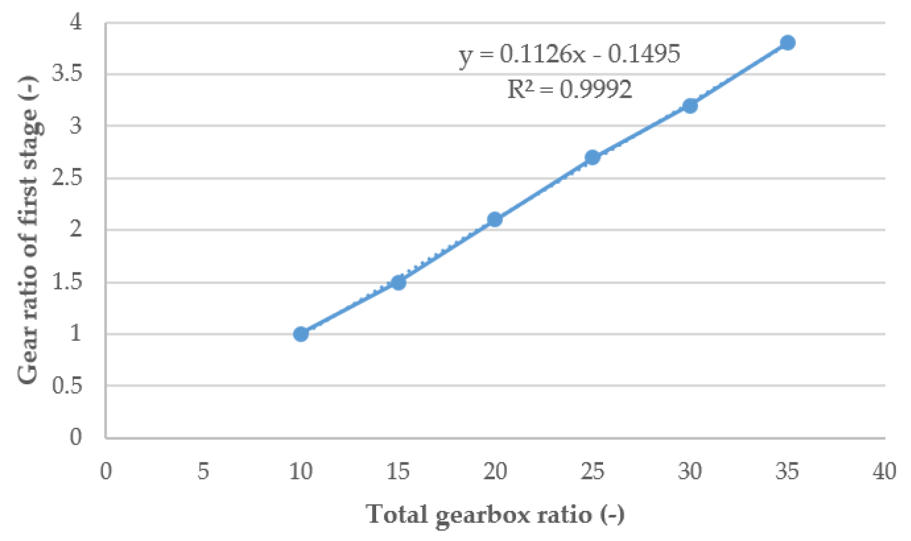
Figure 7 depicts an obvious first-order relationship among the optimal values of u₁ and u_t. Additionally, the following regression equation (with R² = 0.9992) to find the optimal values of u₁ was found:

$$u_1=0.1126·u_t-0.1495$$

(53)

After finding $u_1$, the optimum value of $u_2$ can be determined by $u_2=u_t/u_1$.

To assess the effectiveness of the proposed method, the multi-objective optimization problem was solved using the constraints of u₁, as shown in Table 1 (referred to as the solution by the traditional method). The optimal values for the main design parameters discovered by this method are shown in

Table 11. Optimum main design factors finding by new method.

No.	ut
	10	15	20	25	30	35
u1	1	1.5	2.1	2.7	3.2	3.8
Xba1	0.25	0.2875	0.2875	0.25	0.25	0.25
Xba2	0.25	0.25	0.25	0.25	0.25	0.25
AS1	367.5	420	420	420	420	420
AS2	420	420	420	420	420	420

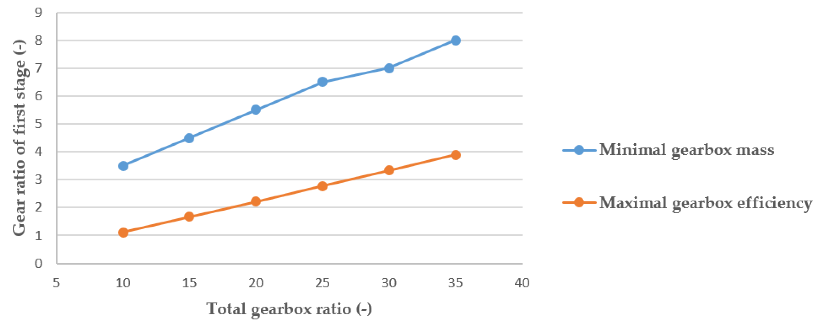
. Figure 8 depicts the optimal values of u₁ as determined by the traditional method (data from Table 10) and the new method (data from Table 9). This figure clearly shows that the optimal values of u₁ for the new method are easily determined and obey a very simple first-order function (Equation (52)). Furthermore, when determined by traditional methods, these values are distributed randomly rather than according to common rules (Figure 8), and they will almost certainly be less accurate than when determined by the new method.

6. Conclusions

The Taguchi method and the GRA are used in this paper to solve the multi-objective optimization problem in designing a two-stage helical gearbox. The goal of the study is to discover the optimal main design parameters that maximize gearbox efficiency while minimizing gearbox mass. To accomplish this, five major design factors were chosen: the CWFW for the first and second stages, the ACS for the first and second stages, and the first-stage gear ratio. In addition, the multi-objective optimization problem is solved in two stages. Phase 1 is concerned with solving the single-objective optimization problem of closing the gap between variable levels, while Phase 2 is concerned with determining the optimal main design factors. The following conclusions were proposed as a result of this work:

-

A novel approach to handling the multi-objective optimization problem in the gearbox design was presented by combining the Taguchi method and the GRA in a two-stage process. The distance between the values of the lower and upper bounds of the constants of u₁ is shortened as a result of this approach, which leads to an easier and a more accurate determination of optimal values.

-

The solution of the single-objective optimization problem bridges the gap between variable levels, making the solution of the multi-objective optimization problem easier and more accurate.

-

From the results of the study, optimal values for the five main design factors in the design of a two-stage helical gear gearbox were proposed (Equation (52) and Table 10).

-

The effect of the main design parameters on $\overline{\mathrm{y}}$ was analyzed using the ANOVA method. The results revealed that AS₂ had the highest influence on $\overline{\mathrm{y}}$ (57.35%), followed by u₁ (25.16%), X_ba1 (5.38%), X_ba2 (2.50%), and AS₁ (0.84%).

-

The proposed model of u₁ demonstrates a high level of consistency with the experimental data, validating their reliability. This model can be effectively utilized for multi-objective optimization of a two-stage helical gearbox, providing a valuable application.

References

1. Patil, M.; Ramkumar, P.; Shankar, K. Multi-objective optimization of the two-stage helical gearbox with tribological constraints. Mech. Mach. Theory 2019, 138, 38–57. [Google Scholar] [CrossRef]
2. Römhild, I.; Linke, H. Gezielte Auslegung Von Zahnradgetrieben mit minimaler Masse auf der Basis neuer Berechnungsverfahren. Konstruktion 1992, 44, 229–236. [Google Scholar]
3. Milou, G.; Dobre, G.; Visa, F.; Vitila, H. Optimal design of two step gear units, regarding the main parameters. VDI Ber. 1996, 1230, 227. [Google Scholar]
4. Pi, V.N. Optimal calculation of partial transmission ratios for four-step helical gearboxes with first and third step double gear-sets for minimal gearbox length. In Proceedings of the American Conference on Applied Mathematics, Cambridge MA, USA, 24–26 March 2008; pp. 29–32. [Google Scholar]
5. Pi, V.N. A new study on optimal calculation of partial transmission ratios of two-step helical gearboxes. In Proceedings of the 2nd WSEAS International Conference on Computer Engineering and Applications, CEA, Acapulco, Mexico, 25–27 January 2008; pp. 162–165. [Google Scholar]
6. Pi, V.N. A new study on the optimal prediction of partial transmission ratios of three-step helical gearboxes with second-step double gear-sets. WSEAS Trans. Appl. Theor. Mech 2007, 2, 156–163. [Google Scholar]
7. Danh, T.H.; Linh, N.H.; Danh, B.T.; Tan, T.M.; Van Trang, N.; Thao, T.T.P.; Cuong, N.M. Effect of Main Design Factors on Two-Stage Helical Gearbox Length. In Proceedings of the Advances in Engineering Research and Application: Proceedings of the International Conference on Engineering Research and Applications, ICERA, Thai Nguyen, Vietnam, 1–2 December 2022; pp. 924–932. [Google Scholar]
8. Pi, V.N. Optimal Calculation of Partial Transmission Ratios of Four-step Helical Gearboxes for Getting Minimal Cross Section Dimension. In Proceedings of the International MultiConference of Engineers and Computer Scientists, Hong Kong, China, 1 January 2008. [Google Scholar]
9. Pi, V.N. A study on optimal determination of partial transmission ratios of helical gearboxes with second-step double gear-sets. Int. J. Mech. Mechatron. Eng. 2008, 2, 26–29. [Google Scholar]
10. Khai, D.Q.; Danh, T.H.; Danh, B.T.; Tan, T.M.; Cuong, N.M.; Hung, L.X.; Pi, V.N.; Thao, T.T.P. Determination of Optimum Main Design Parameters of a Two-Stage Helical Gearbox for Minimum Gearbox Cross-Section Area. In Proceedings of the Advances in Engineering Research and Application: Proceedings of the International Conference on Engineering Research and Applications, ICERA, Thai Nguyen, Vietnam, 1–2 December 2022; pp. 345–353. [Google Scholar]
11. Pi, V.N. Optimal determination of partial transmission ratios for four-step helical gearboxes with first and third step double gear-sets for minimal mass of gears. In Proceedings of the WSEAS International Conference on Applied Computing Conference, Istanbul Turkey, 27–30 May 2008; pp. 53–57. [Google Scholar]
12. Danh, T.H.; Huy, T.Q.; Danh, B.T.; Van Trang, N.; Hung, L.X. Optimization of Main Design Parameters for a Two-Stage Helical Gearbox Based on Gearbox Volume Function. In Proceedings of the Advances in Engineering Research and Application: Proceedings of the International Conference on Engineering Research and Applications, ICERA, Thai Nguyen, Vietnam, 1–2 December 2022; pp. 771–779. [Google Scholar]
13. Vu, N.-P.; Nguyen, D.-N.; Luu, A.-T.; Tran, N.-G.; Tran, T.-H.; Nguyen, V.-C.; Bui, T.-D.; Nguyen, H.-L. The influence of main design parameters on the overall cost of a gearbox. Appl. Sci. 2020, 10, 2365. [Google Scholar] [CrossRef] [Green Version]
14. Quang, N.H.; Tu, N.T.; Linh, N.H.; Luan, N.H.; Anh, L.H.; Tuan, N.A.; Giang, T.N.; Pi, V.N. Determining Optimum Gear Ratios for a Four-Stage Helical Gearbox for Getting Minimum Gearbox Cost. In Proceedings of the Advances in Engineering Research and Application: Proceedings of the International Conference on Engineering Research and Applications, ICERA, Thai Nguyen, Vietnam, 1–2 December 2021; pp. 350–364. [Google Scholar]
15. Danh, T.H.; Huy, T.Q.; Danh, B.T.; Tan, T.M.; Van Trang, N.; Tung, L.A. Determining Partial Gear Ratios of a Two-Stage Helical Gearbox with First Stage Double Gear Sets for Minimizing Total Gearbox Cost. In Proceedings of the Advances in Engineering Research and Application: Proceedings of the International Conference on Engineering Research and Applications, ICERA, Thai Nguyen, Vietnam, 1–2 December 2022; pp. 376–388. [Google Scholar]
16. Anh, L.H.; Linh, N.H.; Quang, N.H.; Duc Lam, P.; Anh Tuan, N.; Khac Tuan, N.; Thi Thanh Nga, N.; Ngoc Pi, V. Cost optimization of two-stage helical gearboxes with second stage double gear-sets. EUREKA Phys. Eng. 2021, 89–101. [Google Scholar] [CrossRef]
17. Wu, Y.-R.; Tran, V.-T. Transmission and load analysis for a crowned helical gear pair with twist-free tooth flanks generated by an external gear honing machine. Mech. Mach. Theory 2016, 98, 36–47. [Google Scholar] [CrossRef]
18. Gologlu, C.; Zeyveli, M. A genetic approach to automate preliminary design of gear drives. Comput. Ind. Eng. 2009, 57, 1043–1051. [Google Scholar] [CrossRef]
19. Thompson, D.F.; Gupta, S.; Shukla, A. Tradeoff analysis in minimum volume design of multi-stage spur gear reduction units. Mech. Mach. Theory 2000, 35, 609–627. [Google Scholar] [CrossRef]
20. Maputi, E.S.; Arora, R. Multi-objective optimization of a 2-stage spur gearbox using NSGA-II and decision-making methods. J. Braz. Soc. Mech. Sci. Eng. 2020, 42, 477. [Google Scholar] [CrossRef]
21. Sanghvi, R.C.; Vashi, A.S.; Patolia, H.; Jivani, R.G. Multi-objective optimization of two-stage helical gear train using NSGA-II. J. Optim. 2014, 2014, 670297. [Google Scholar] [CrossRef] [Green Version]
22. Park, C.I. Multi-objective optimization of the tooth surface in helical gears using design of experiment and the response surface method. J. Mech. Sci. Technol. 2010, 24, 823–829. [Google Scholar] [CrossRef]
23. Chat, T.; Van Uyen, L. Design and Calculation of Mechanical Transmissions Systems; Educational Republishing House: Hanoi, Vietnam, 2007; Volume 1. [Google Scholar]
24. SKF Group, Roller Bearings. 2018. Available online: https://www.skf.com/binaries/pub12/Images/0901d196802809de-Rolling-bearings---17000_1-EN_tcm_12-121486.pdf (accessed on 24 May 2023).
25. Jelaska, D.T. Gears and Gear Drives; John Wiley & Sons: Hoboken, NJ, USA, 2012. [Google Scholar]
26. Buckingham, E. Analytical Mechanics of Gears; Dover Publications, Inc.: New York, NY, USA, 1988. [Google Scholar]
Figure 2. Diagram for determining shaft dimensions.
Applsci 13 07601 g002
Figure 3. The procedure for solving a multi-objective problem.
Applsci 13 07601 g003
Figure 4. Gear ratio of the first stage versus total gearbox ratio.
Applsci 13 07601 g004
Figure 5. Influence of main design factors on S/N ratios of y ¯ .
Applsci 13 07601 g005
Figure 6. Probability plot of y ¯ .
Applsci 13 07601 g006
Figure 7. Optimal gear ratio of the first stage versus total gearbox ratio.
Applsci 13 07601 g007
Figure 8. Optimal gear ratio of first stage of traditional and new method.
Applsci 13 07601 g008