

Development and Integration of a Workpiece-Based Calibration Method for an Optical Assistance System


Abstract
:1. Introduction
1.1. Motivation
1.2. Research Gap
1.3. Outline of This Work
2. State of the Art and Related Work
2.1. Assistance Systems
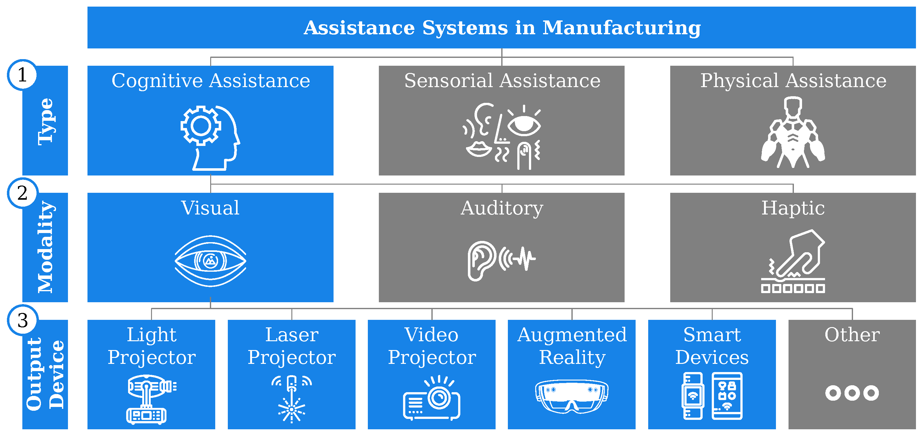
2.1.1. Classification of Assistance Systems in Manufacturing
2.1.2. Cognitive Assistance Systems
2.2. Commissioning of Visual Light Projectors
2.3. Workpiece-Based Referencing
3. Fundamentals: Workpiece and Moving Head Kinematics
3.1. Axis and Control of the Moving Head
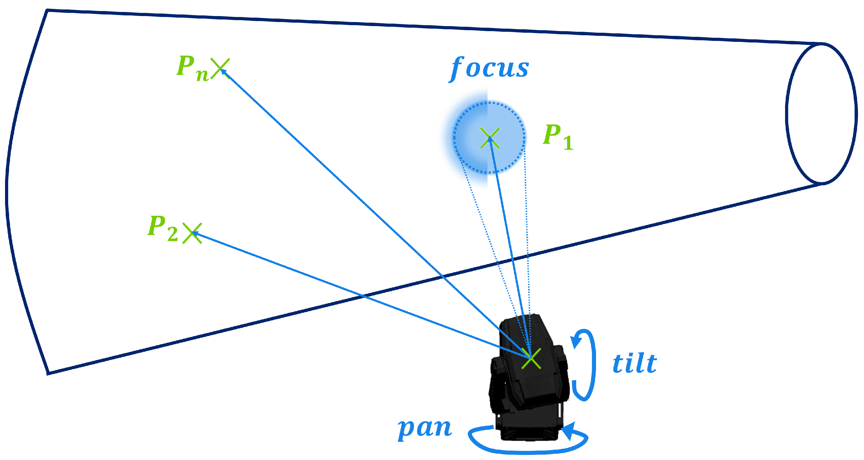
3.1.1. Pan and Tilt
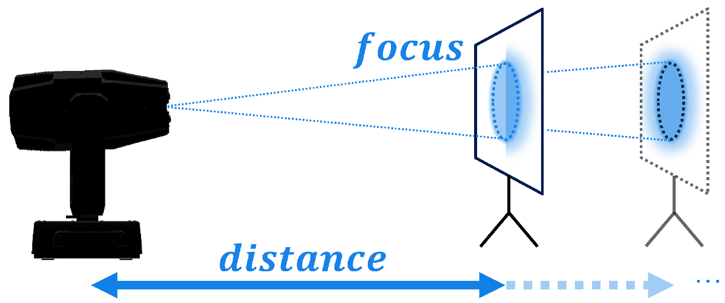
3.1.2. Focus
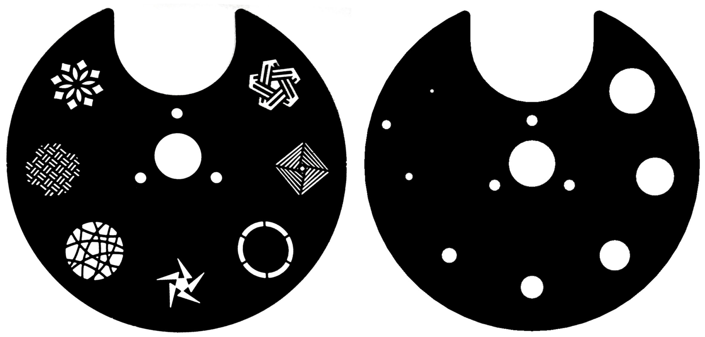
3.1.3. Gobo Wheels
3.2. Control with Cartesian Coordinates
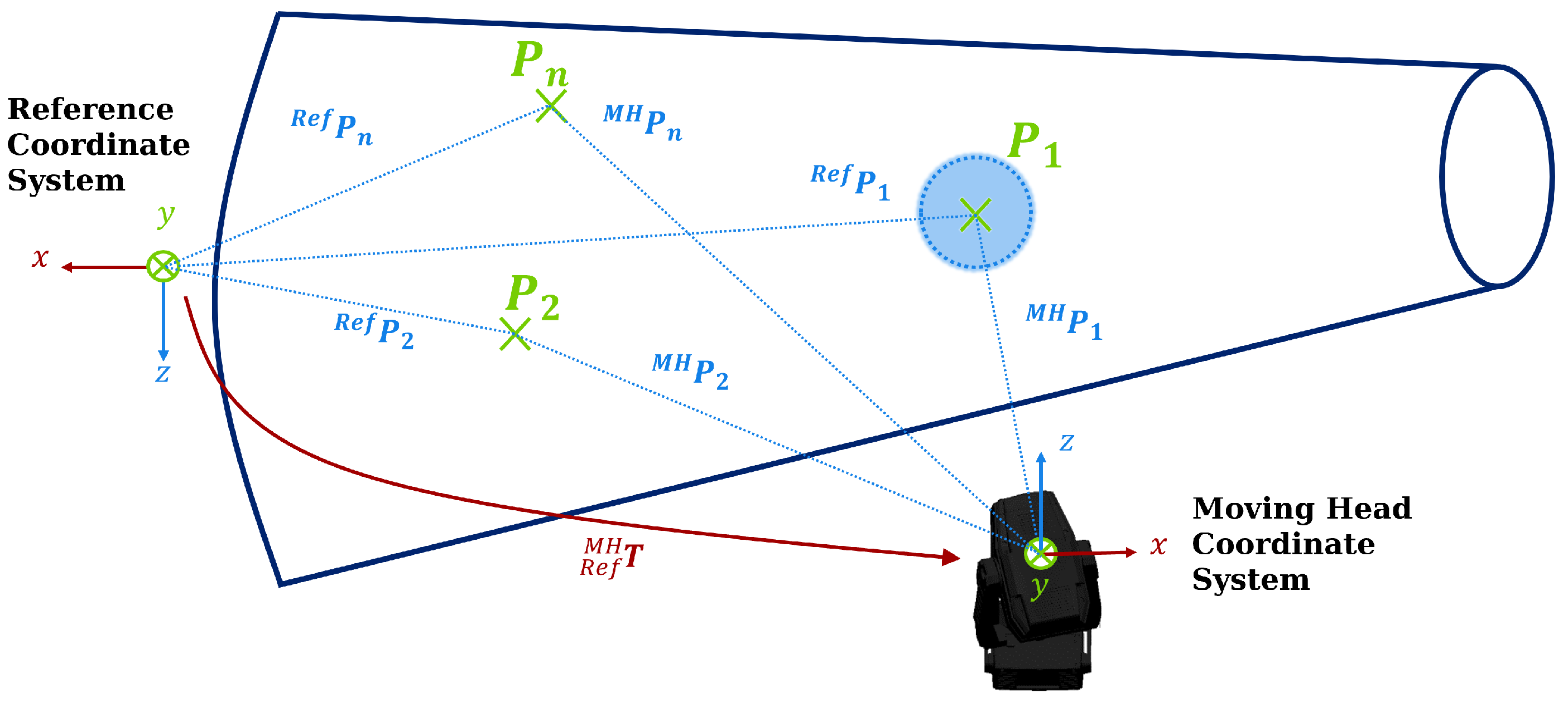
3.3. Coordinate Systems and Transformations
3.4. Usage of Non-Linear, Multidimensional Newton’s Method
- 1.
- The zero has been found with sufficient accuracy:This condition does not guarantee convergence but can be used if convergence is not a requirement.
- 2.
- The difference between two x values fell below a specified threshold:This condition signifies convergence but does not guarantee the zero has been found accurately.
- 3.
- The maximum iteration step count K has been reached without fulfilling one of the other criteria. This usually means the iteration did not converge, or that it oscillates around the zero.
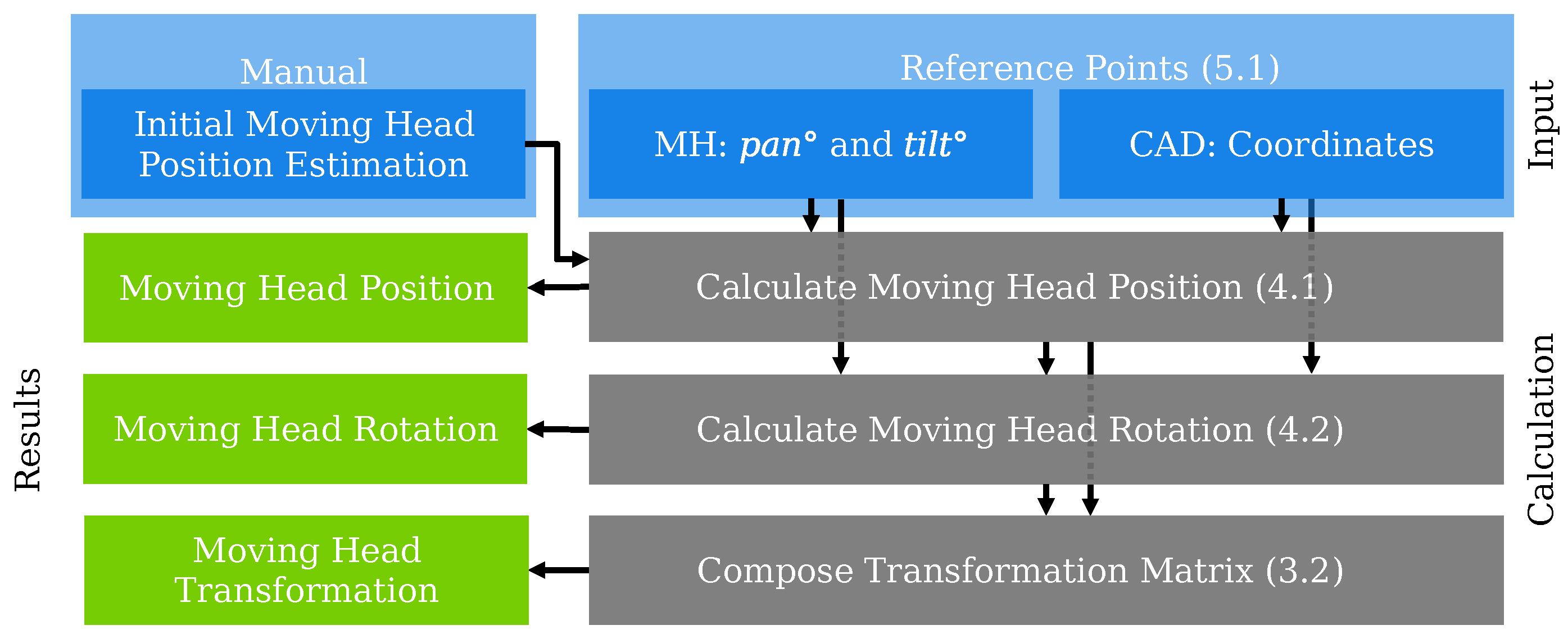
4. Moving Head Calibration
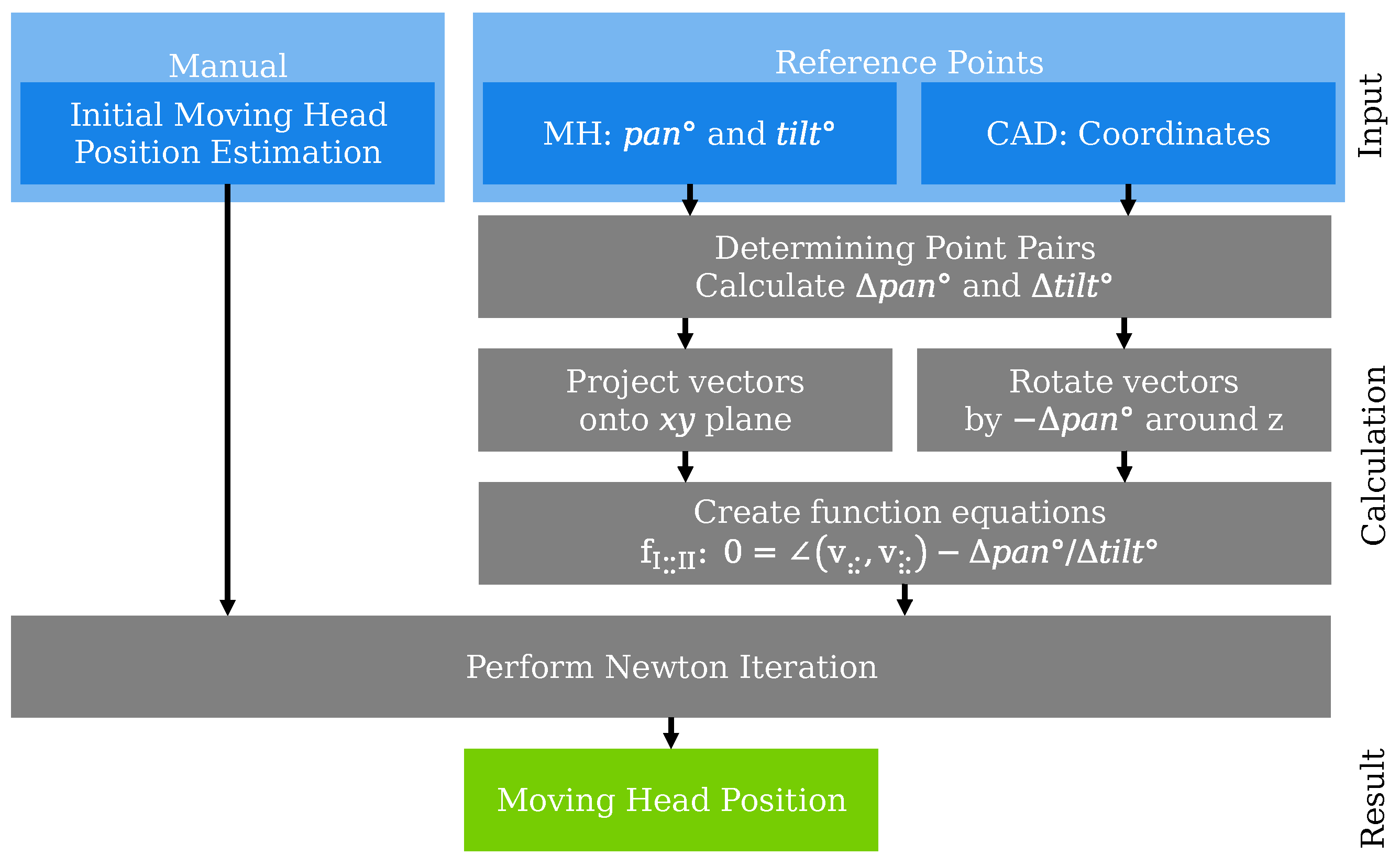
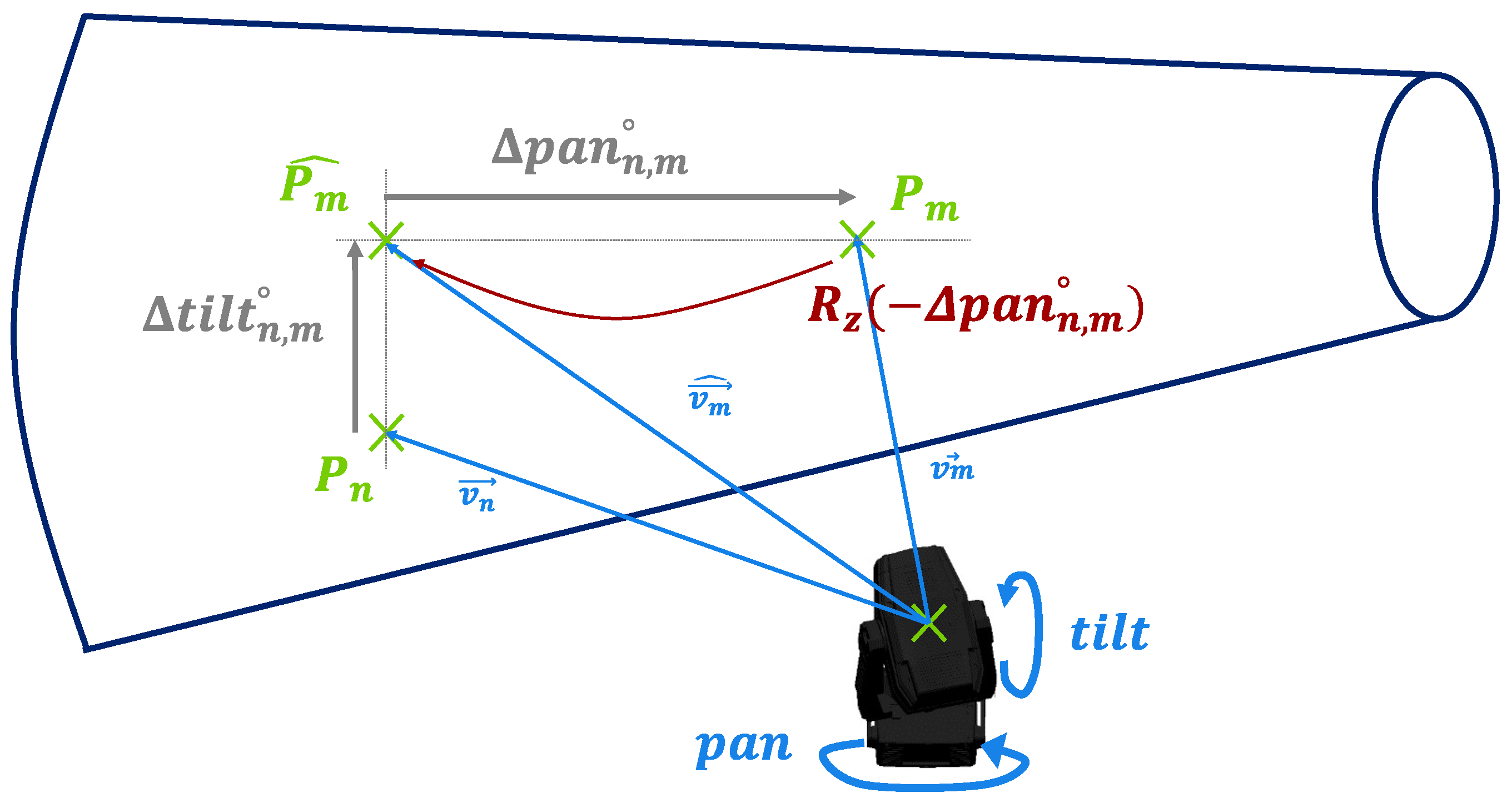
4.1. Determining the Moving Head Position
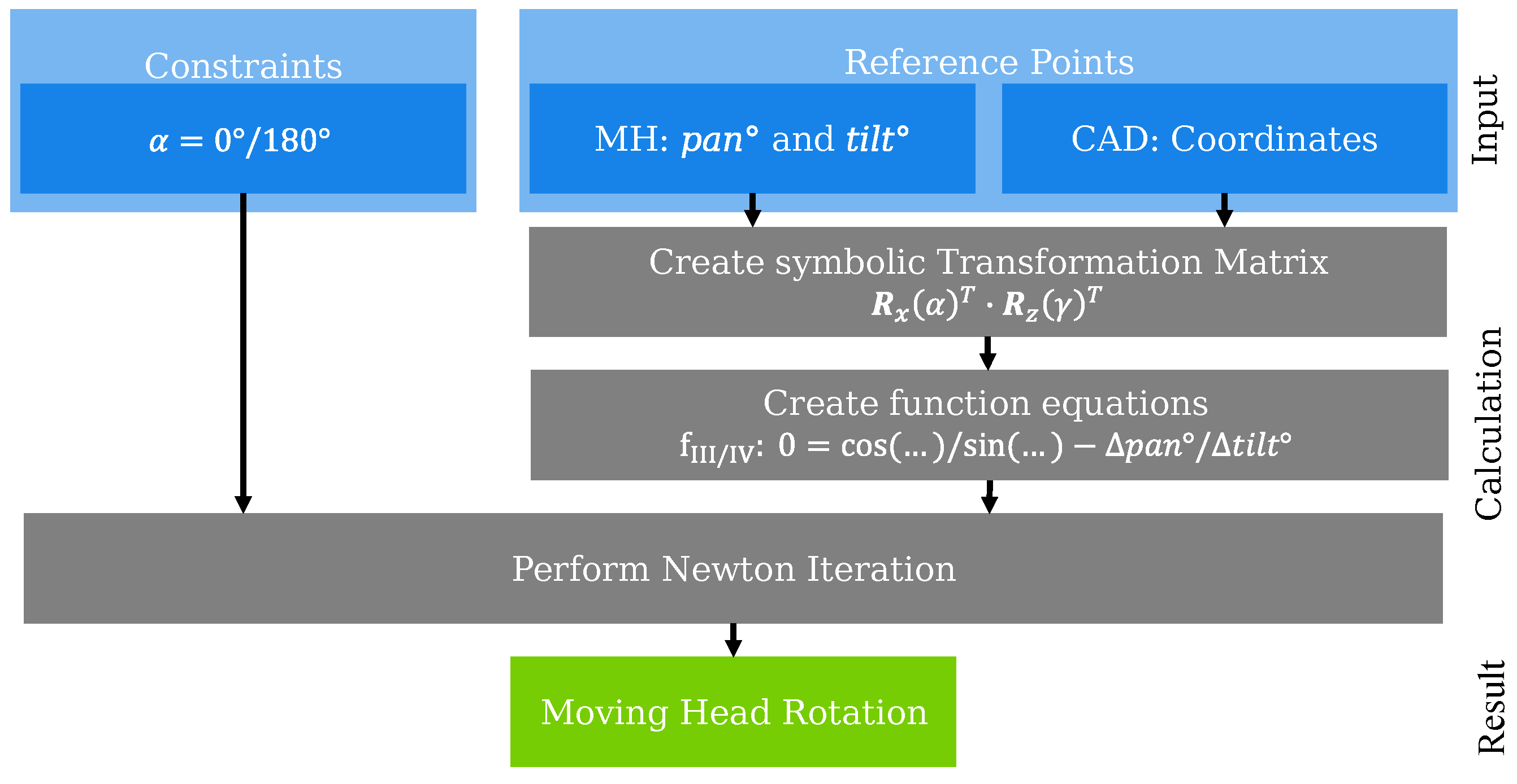
4.2. Determining the Moving Head Orientation
5. Validation
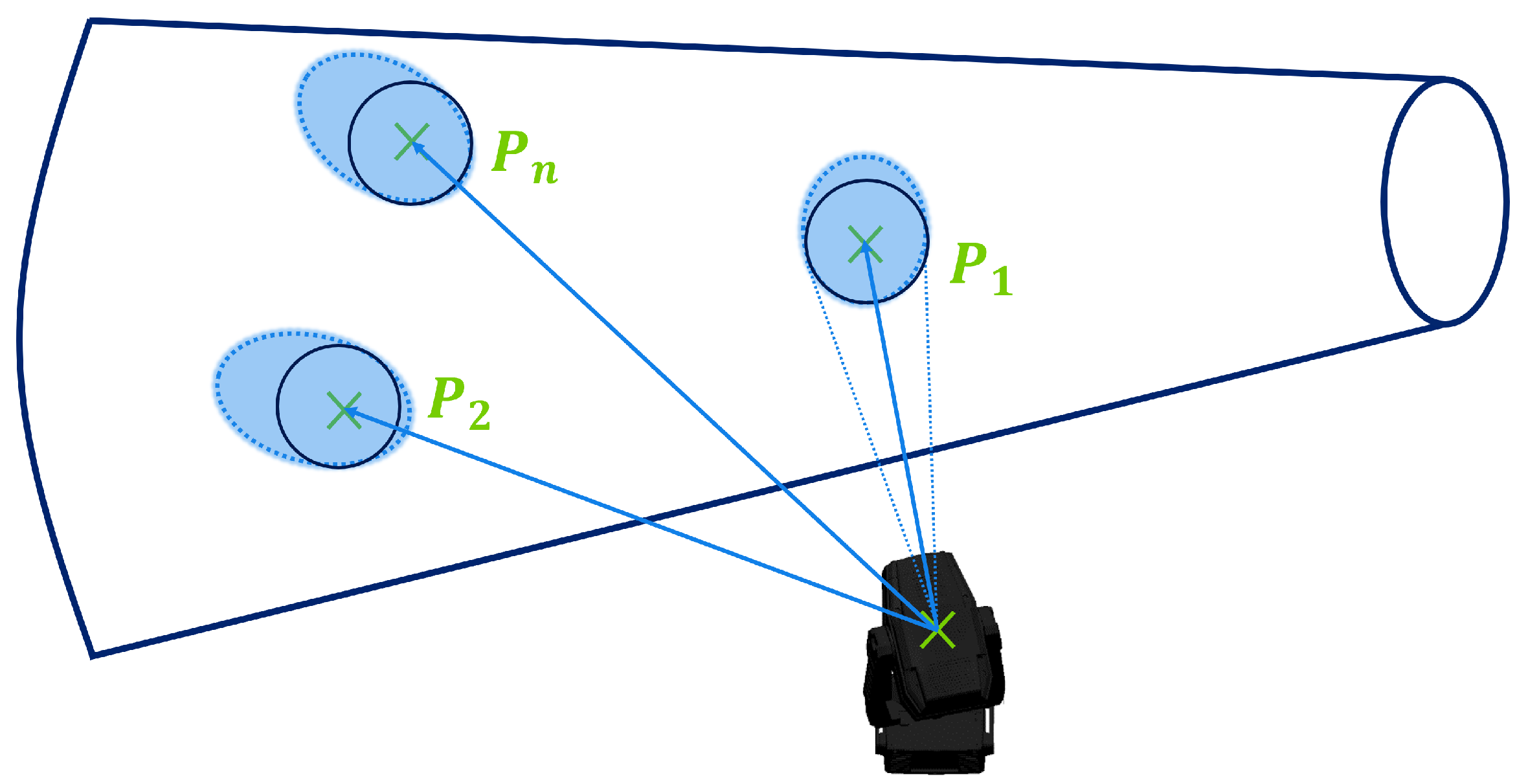
5.1. Capturing Reference Points
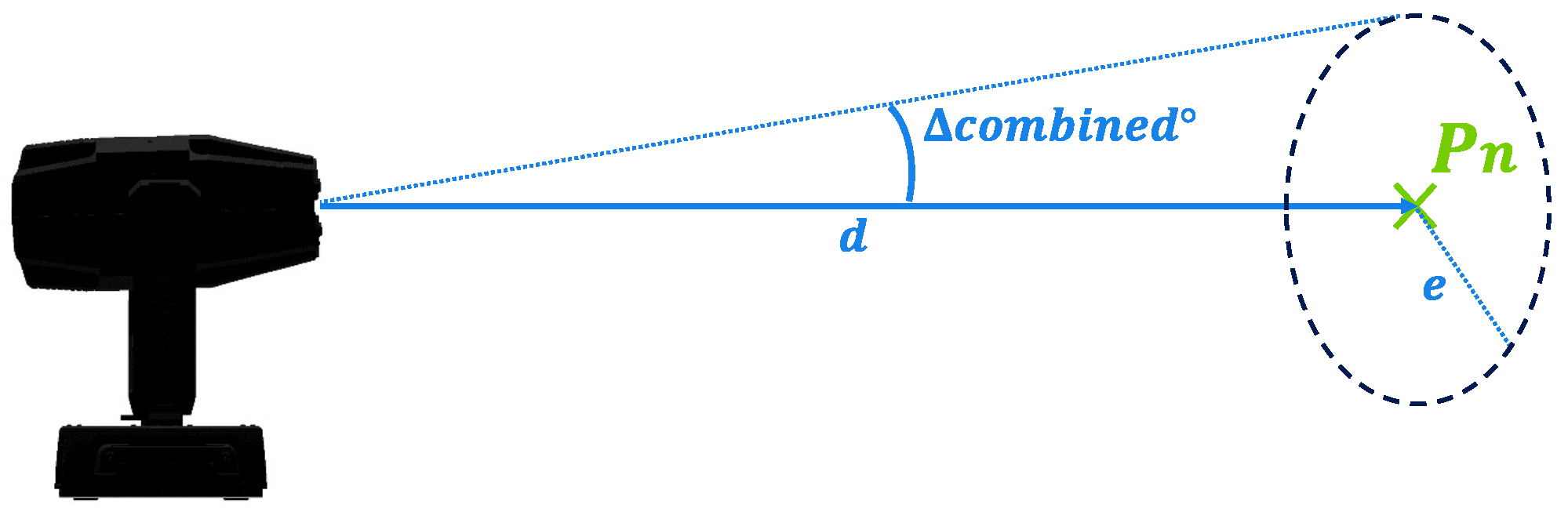
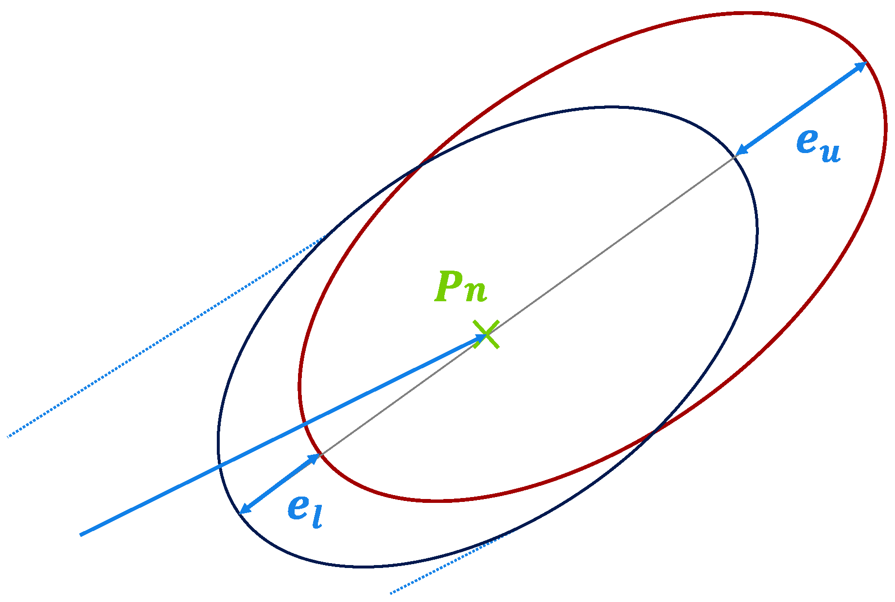
5.2. Theoretical and Mechanical Limits
5.3. Algorithmic Accuracy
5.4. Practical Validation
6. Discussion
7. Summary
8. Outlook and Future Work
Author Contributions
Funding
Institutional Review Board Statement
Informed Consent Statement
Data Availability Statement
Conflicts of Interest
Appendix A. Control of the Moving Head with Node-RED
Appendix A.1. Data Flow and Communication Overview

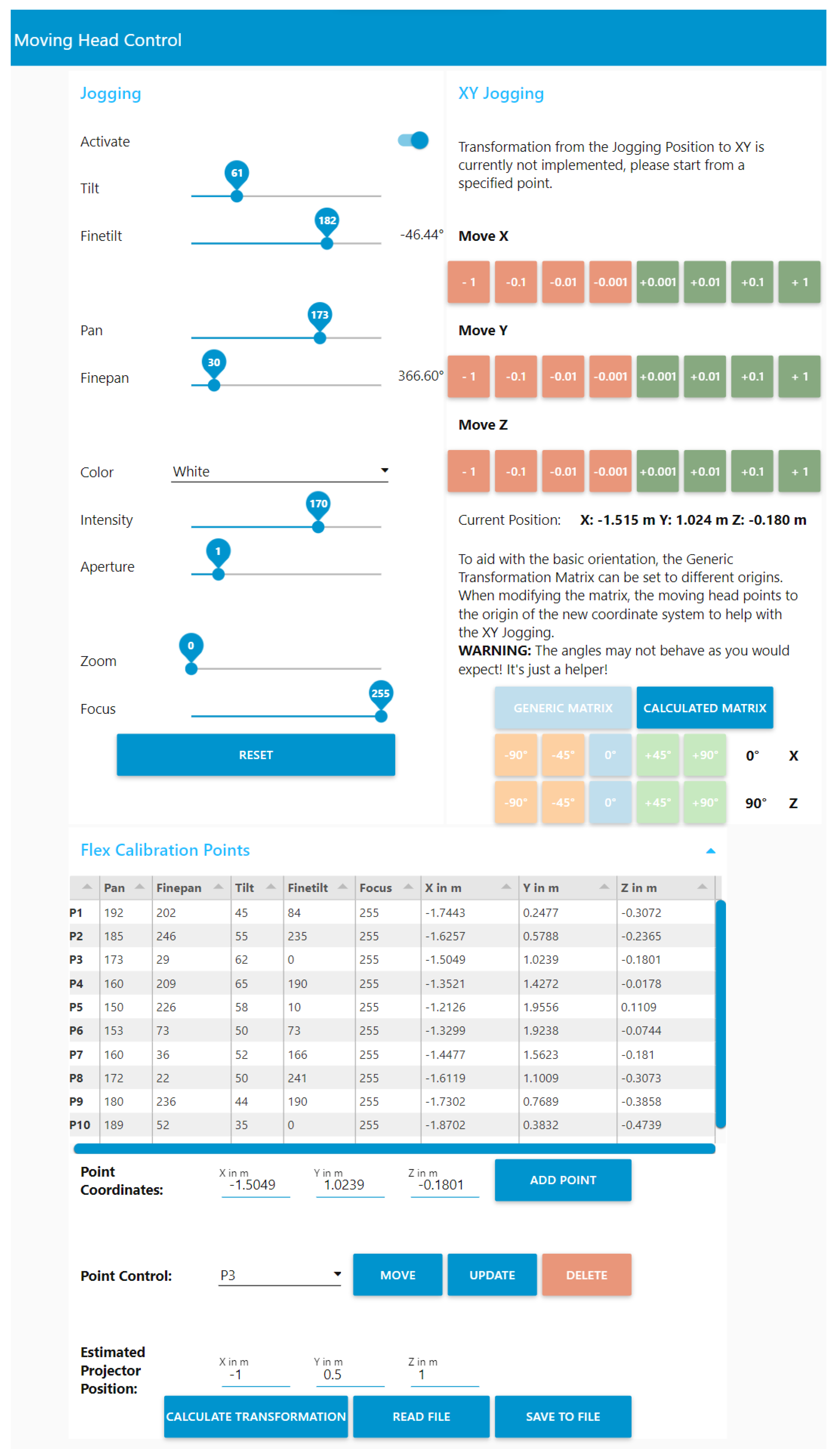
Appendix A.2. The Node-RED Dashboard

Appendix B. Special Remarks on the Moving Head
Appendix B.1. Control of the Pan and Tilt Axis
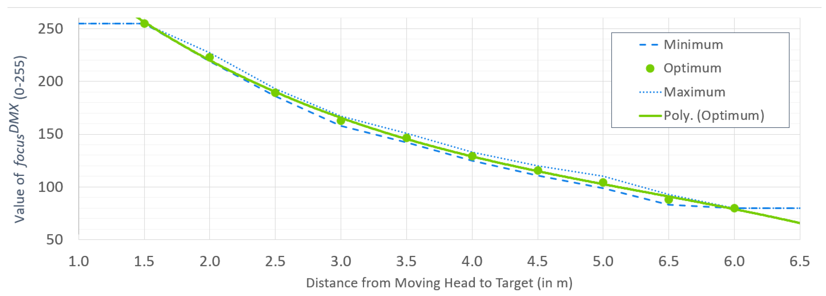
Appendix B.2. Control of the Focus


| Distance | Minimum | Optimum | Maximum |
|---|---|---|---|
| ≤1.0 | 255 | 255 | 255 |
| 1.5 | 255 | 255 | 255 |
| 2.0 | 219 | 223 | 227 |
| 2.5 | 186 | 189.5 | 193 |
| 3.0 | 158 | 162.5 | 167 |
| 3.5 | 142 | 146.5 | 151 |
| 4.0 | 125 | 129 | 133 |
| 4.5 | 111 | 115.5 | 120 |
| 5.0 | 99 | 104.5 | 110 |
| 6.5 | 83 | 88 | 93 |
| ≥6.0 | 80 | 80 | 80 |
Appendix B.3. Behaviour of the Gobo Wheel
Appendix C. Validation Data
Appendix C.1. Reference Points and Calibration Results
| Index | pan | finepan | tilt | finetilt | X in m | Y in m | Z in m | in mm | in mm |
|---|---|---|---|---|---|---|---|---|---|
| 1 | 192 | 202 | 45 | 84 | −1.7443 | 0.2477 | −0.3072 | 5 | 5 |
| 2 | 185 | 246 | 55 | 235 | −1.6257 | 0.5788 | −0.2365 | 3 | 6 |
| 3 | 173 | 29 | 62 | 0 | −1.5049 | 1.0239 | −0.1801 | 3 | 4 |
| 4 | 160 | 209 | 65 | 190 | −1.3521 | 1.4272 | −0.0178 | 3 | 3 |
| 5 | 150 | 226 | 58 | 10 | −1.2126 | 1.9556 | 0.1109 | 4 | 6 |
| 6 | 153 | 73 | 50 | 73 | −1.3299 | 1.9238 | −0.0744 | 3 | 6 |
| 7 | 160 | 36 | 52 | 166 | −1.4477 | 1.5623 | −0.1810 | 6 | 6 |
| 8 | 172 | 22 | 50 | 241 | −1.6119 | 1.1009 | −0.3073 | 5 | 6 |
| 9 | 180 | 236 | 44 | 190 | −1.7302 | 0.7689 | −0.3858 | 4 | 4 |
| 10 | 189 | 52 | 35 | 0 | −1.8702 | 0.3832 | −0.4739 | 5 | 5 |
| 11 | 160 | 170 | 45 | 225 | −1.5453 | 1.6221 | −0.2528 | 5 | 5 |
| 4.18 | 5.09 | ||||||||
| 4.64 | |||||||||
| 1.03 | 1.00 | ||||||||
| 0.83 |
Appendix C.2. Pose Repeatability Measurements
| Index | X in mm | Y in mm | Z in mm | in mm |
|---|---|---|---|---|
| 1 | −306.4154 | −2032.1464 | −972.1941 | 0.00188634 |
| 2 | −306.4316 | −2032.1124 | −972.2038 | 0.00220966 |
| 3 | −306.2175 | −2032.1691 | −971.9397 | 0.00263319 |
| 4 | −306.2847 | −2032.1653 | −971.9680 | 0.00199971 |
| 5 | −306.2746 | −2032.1472 | −971.9647 | 0.00221153 |
| 6 | −306.2349 | −2032.1175 | −971.9473 | 0.00211342 |
| 7 | −306.2486 | −2032.1570 | −971.9434 | 0.00228444 |
| 8 | −306.2201 | −2032.1406 | −971.9422 | 0.00236737 |
| −306.290925 | −2032.144438 | −972.0129 | 0.002213208 | |
| 0.079785928 | 0.019298765 | 0.107880628 | 0.000214366 |
Appendix C.3. Remarks on the Performance of Newton’s Method

References
- Froschauer, R.; Kurschl, W.; Wolfartsberger, J.; Pimminger, S.; Lindorfer, R.; Blattner, J. A Human-Centered Assembly Workplace For Industry: Challenges and Lessons Learned. Procedia Comput. Sci. 2021, 180, 290–300. [Google Scholar] [CrossRef]
- Maddikunta, P.K.R.; Pham, Q.V.; B, P.; Deepa, N.; Dev, K.; Gadekallu, T.R.; Ruby, R.; Liyanage, M. Industry 5.0: A survey on enabling technologies and potential applications. J. Ind. Inf. Integr. 2022, 26, 100257. [Google Scholar] [CrossRef]
- Bornewasser, M.; Hinrichsen, S. (Eds.) Informatorische Assistenzsysteme in der Variantenreichen Montage: Theorie und Praxis; Springer: Berlin/Heidelberg, Germany, 2020. [Google Scholar] [CrossRef]
- Mark, B.G.; Rauch, E.; Matt, D.T. Industrial Assistance Systems to Enhance Human–Machine Interaction and Operator’s Capabilities in Assembly. In Implementing Industry 4.0 in SMEs: Concepts, Examples and Applications; Matt, D.T., Modrák, V., Zsifkovits, H., Eds.; Springer: Cham, Switzerland, 2021; pp. 129–161. [Google Scholar] [CrossRef]
- Kalscheuer, F.; Eschen, H.; Schüppstuhl, T. Towards Semi Automated Pre-assembly for Aircraft Interior Production. In Annals of Scientific Society for Assembly, Handling and Industrial Robotics 2021; Schüppstuhl, T., Ed.; Springer: Cham, Switzerland, 2022; pp. 203–213. [Google Scholar] [CrossRef]
- Mark, B.G.; Rauch, E.; Matt, D.T. Worker assistance systems in manufacturing: A review of the state of the art and future directions. J. Manuf. Syst. 2021, 59, 228–250. [Google Scholar] [CrossRef]
- Müller, R.; Hörauf, L.; Vette-Steinkamp, M.; Kanso, A.; Koch, J. The Assist-By-X system: Calibration and application of a modular production equipment for visual assistance. Procedia CIRP 2019, 86, 179–184. [Google Scholar] [CrossRef]
- Schoepflin, D.; Koch, J.; Gomse, M.; Schüppstuhl, T. Smart Material Delivery Unit for the Production Supplying Logistics of Aircraft. Procedia Manuf. 2021, 55, 455–462. [Google Scholar] [CrossRef]
- Hinrichsen, S.; Adrian, B.; Bornewasser, M. Information Management Strategies in Manual Assembly. In Human Interaction, Emerging Technologies and Future Applications II, Proceedings of the 2nd International Conference on Human Interaction and Emerging Technologies: Future Applications (IHIET—AI 2020), Lausanne, Switzerland, 23–25 April 2020; Ahram, T., Taiar, R., Gremeaux-Bader, V., Aminian, K., Eds.; Advances in Intelligent Systems and Computing; Springer: Cham, Switzerland, 2020; Volume 1152, pp. 520–525. [Google Scholar] [CrossRef]
- Romero, D.; Bernus, P.; Noran, O.; Stahre, J.; Fast-Berglund, Å. The Operator 4.0: Human Cyber-Physical Systems & Adaptive Automation Towards Human-Automation Symbiosis Work Systems. In Advances in Production Management Systems. Initiatives for a Sustainable World, Proceedings of the IFIP WG 5.7 International Conference, APMS 2016, Iguassu Falls, Brazil, 3–7 September 2016; Nääs, I.A., Vendrametto, O., Mendes Reis, J., Gonçalves, R.F., Terra Silva, M., von Cieminski, G., Kiritsis, D., Eds.; IFIP Advances in Information and Communication Technology; Springer: Cham, Switzerland, 2016; Volume 488, pp. 677–686. [Google Scholar] [CrossRef] [Green Version]
- Müller, R.; Vette-Steinkamp, M.; Hörauf, L.; Speicher, C.; Bashir, A. Worker centered cognitive assistance for dynamically created repairing jobs in rework area. Procedia CIRP 2018, 72, 141–146. [Google Scholar] [CrossRef]
- Koch, J.; Büsch, L.; Gomse, M.; Schüppstuhl, T. A Methods-Time-Measurement based Approach to enable Action Recognition for Multi-Variant Assembly in Human-Robot Collaboration. Procedia CIRP 2022, 106, 233–238. [Google Scholar] [CrossRef]
- Keller, T.; Bayer, C.; Bausch, P.; Metternich, J. Benefit evaluation of digital assistance systems for assembly workstations. Procedia CIRP 2019, 81, 441–446. [Google Scholar] [CrossRef]
- Petzoldt, C.; Keiser, D.; Beinke, T.; Freitag, M. Functionalities and Implementation of Future Informational Assistance Systems for Manual Assembly. In Subject-Oriented Business Process Management. The Digital Workplace—Nucleus of Transformation, Proceedings of the 12th International Conference, S-BPM ONE 2020, Bremen, Germany, 2–3 December 2020; Freitag, M., Kinra, A., Kotzab, H., Kreowski, H.J., Thoben, K.D., Eds.; Springer: Cham, Switzerland, 2020; Volume 1278, pp. 88–109. [Google Scholar] [CrossRef]
- Weidner, R.; Karafillidis, A.; Wulfsberg, J.P. Individual Support in Industrial Production—Outline of a Theory of Support-Systems. In Proceedings of the 49th Annual Hawaii International Conference on System Sciences (HICSS), Koloa, HI, USA, 5–8 January 2016; Bui, T.X., Sprague, R.H., Eds.; IEEE: Piscataway, NJ, USA, 2016; pp. 569–578. [Google Scholar] [CrossRef]
- Gualtieri, L.; Palomba, I.; Wehrle, E.J.; Vidoni, R. The Opportunities and Challenges of SME Manufacturing Automation: Safety and Ergonomics in Human–Robot Collaboration. In Industry 4.0 for SMEs: Challenges, Opportunities and Requirements; Matt, D., Modrak, V., Zsifkovits, H.E., Eds.; Palgrave Macmillan: Cham, Switzerland, 2020; pp. 105–144. [Google Scholar] [CrossRef] [Green Version]
- Masiak, T. Entwicklung eines Mensch-Roboter-kollaborationsfähigen Nietprozesses unter Verwendung von KI-Algorithmen und Blockchain-Technologien: Unter Randbedingungen der Flugzeugstrukturmontage. Ph.D. Thesis, Saarland University, Saarbrücken, Germany, 2020. [Google Scholar] [CrossRef]
- Neßelrath, R. SiAM-dp: An open development platform for massively multimodal dialogue systems in cyber-physical environments. Ph.D. Thesis, Saarland University, Saarbrücken, Germany, 2015. [Google Scholar] [CrossRef]
- Neumann, A.; Strenge, B.; Uhlich, J.C.; Schlicher, K.D.; Maier, G.W.; Schalkwijk, L.; Waßmuth, J.; Essig, K.; Schack, T. AVIKOM—Towards a Mobile Audiovisual Cognitive Assistance System for Modern Manufacturing and Logistics. In Proceedings of the 13th ACM International Conference on PErvasive Technologies Related to Assistive Environments, Corfu, Greece, 30 June–3 July 2020; Makedon, F., Ed.; Association for Computing Machinery: New York, NY, USA, 2020; pp. 1–8. [Google Scholar] [CrossRef]
- Borisov, N.; Weyers, B.; Kluge, A. Designing a Human Machine Interface for Quality Assurance in Car Manufacturing: An Attempt to Address the “Functionality versus User Experience Contradiction” in Professional Production Environments. Adv. Hum.-Comput. Interact. 2018, 2018, 1–18. [Google Scholar] [CrossRef]
- Hold, P.; Erol, S.; Reisinger, G.; Sihn, W. Planning and Evaluation of Digital Assistance Systems. Procedia Manuf. 2017, 9, 143–150. [Google Scholar] [CrossRef]
- Sochor, R.; Kraus, L.; Merkel, L.; Braunreuther, S.; Reinhart, G. Approach to Increase Worker Acceptance of Cognitive Assistance Systems in Manual Assembly. Procedia CIRP 2019, 81, 926–931. [Google Scholar] [CrossRef]
- Hinrichsen, S.; Riediger, D.; Unrau, A. Development of a projection-based assistance system for maintaining injection molding tools. In Proceedings of the 2017 IEEE International Conference on Industrial Engineering & Engineering Management (IEEM), Singapore, Singapore, 10–13 December 2017; pp. 1571–1575. [Google Scholar] [CrossRef]
- Eversberg, L.; Ebrahimi, P.; Pape, M.; Lambrecht, J. A cognitive assistance system with augmented reality for manual repair tasks with high variability based on the digital twin. Manuf. Lett. 2022, 34, 49–52. [Google Scholar] [CrossRef]
- Deneke, C.; Moenck, K.; Schueppstuhl, T. Augmented Reality Based Data Improvement for the Planning of Aircraft Cabin Conversions. In Proceedings of the 2021 The 8th International Conference on Industrial Engineering and Applications (Europe), Barcelona, Spain, 8–11 January 2021; Association for Computing Machinery: New York, NY, USA, 2021; pp. 37–45. [Google Scholar] [CrossRef]
- Sidiropoulos, V.; Bechtsis, D.; Vlachos, D. An Augmented Reality Symbiosis Software Tool for Sustainable Logistics Activities. Sustainability 2021, 13, 10929. [Google Scholar] [CrossRef]
- Dolgov, O.S.; Kolosov, A.I.; Safoklov, B.B. Study of the Effectiveness of the Introduction of Laser Projection System in the Process of Technological Preparation of the Production of Aircraft Structures From Polymer Composite Materials. In Proceedings of the 2021 International Ural Conference on Electrical Power Engineering (UralCon), Magnitogorsk, Russia, 24–26 September 2021; pp. 639–643. [Google Scholar] [CrossRef]
- Rupprecht, P.; Kueffner-Mccauley, H.; Schlund, S. Information provision utilizing a dynamic projection system in industrial site assembly. Procedia CIRP 2020, 93, 1182–1187. [Google Scholar] [CrossRef]
- Bertram, P. Entwicklung Eines Kontextsensitiven, Modularen Assistenzsystems für Manuelle Tätigkeiten, 1st ed.; Mensch-Maschine-Systeme Series; VDI Verlag: Düsseldorf, Germany, 2020; Volume 40. [Google Scholar] [CrossRef]
- Eschen, H.; Kötter, T.; Rodeck, R.; Harnisch, M.; Schüppstuhl, T. Augmented and Virtual Reality for Inspection and Maintenance Processes in the Aviation Industry. Procedia Manuf. 2018, 19, 156–163. [Google Scholar] [CrossRef]
- Wang, X.; Ong, S.K.; Nee, A.Y.C. A comprehensive survey of augmented reality assembly research. Adv. Manuf. 2016, 4, 1–22. [Google Scholar] [CrossRef]
- Martin, P.; Marchand, E.; Houlier, P.; Marchal, I. Mapping and re-localization for mobile augmented reality. In Proceedings of the 2014 IEEE International Conference on Image Processing (ICIP 2014), Paris, France, 27–30 October 2014; pp. 3352–3356. [Google Scholar] [CrossRef] [Green Version]
- Vovk, A.; Wild, F.; Guest, W.; Kuula, T. Simulator Sickness in Augmented Reality Training Using the Microsoft HoloLens. In Proceedings of the 2018 CHI Conference on Human Factors in Computing Systems, Montreal, QC, Canada, 21–26 April 2018; Mandryk, R., Ed.; Association for Computing Machinery: New York, NY, USA, 2018; pp. 1–9. [Google Scholar] [CrossRef]
- Hinrichsen, S.; Bornewasser, M. How to Design Assembly Assistance Systems. In Intelligent Human Systems Integration 2019, Proceedings of the 2nd International Conference on Intelligent Human Systems Integration (IHSI 2019): Integrating People and Intelligent Systems, San Diego, CA, USA, 7–10 February 2019; Advances in Intelligent Systems and Computing; Karwowski, W., Ahram, T., Eds.; Springer: Cham, Switzerland, 2019; Volume 903, pp. 286–292. [Google Scholar] [CrossRef]
- Pokorni, B.; Popescu, D.; Constantinescu, C. Design of Cognitive Assistance Systems in Manual Assembly Based on Quality Function Deployment. Appl. Sci. 2022, 12, 3887. [Google Scholar] [CrossRef]
- Denavit, J.; Hartenberg, R.S. A Kinematic Notation for Lower-Pair Mechanisms Based on Matrices. J. Appl. Mech. 1955, 22, 215–221. [Google Scholar] [CrossRef]
- Yongguo, Z.; Xiang, H.; Wei, F.; Shuanggao, L. Trajectory Planning Algorithm Based on Quaternion for 6-DOF Aircraft Wing Automatic Position and Pose Adjustment Method. Chin. J. Aeronaut. 2010, 23, 707–714. [Google Scholar] [CrossRef] [Green Version]
- Sutton, B. Chapter 31: Newton’s method. In Numerical Analysis: Theory and Experiments; Sutton, B., Ed.; Society for Industrial and Applied Mathematics: Philadelphia, PA, USA, 2019; pp. 347–359. [Google Scholar] [CrossRef]
- Higham, N.J. Chapter 25: Nonlinear Systems and Newton’s Method. In Accuracy and Stability of Numerical Algorithms; Higham, N.J., Ed.; Society for Industrial and Applied Mathematics: Philadelphia, PA, USA, 2002; pp. 459–469. [Google Scholar] [CrossRef]
- Leica Geosystems AG. Leica Laser Tracker for Hand-Tools: Superior by Any Measure—LT(D)800: Document 731 982—III. 2003. Available online: https://www.sigma3d.de/fileadmin/Webseiten-Daten/Dokumente/VermietungProduktPDFs/Vermietung_Lasertracker_Leica_LT_D_800.pdf (accessed on 20 April 2023).
- ISO 9283:1998; Manipulating Industrial Robots: Performance Criteria and Related Test Methods. International Organization for Standardization: Geneva, Switzerland, 1998.
- Highlite International B.V. Showtec Phantom 130 Spot V1 Manual. Available online: https://www.highlite.com/media/attachments/MANUAL/40073_MANUAL_GB_V1.pdf (accessed on 4 June 2023).
- ENTTEC Ltd. Open DMX Ethernet Mk2—RDM Compliant DMX Over Ethernet Gateway. Available online: https://support.enttec.com/helpdesk/attachments/101026597782 (accessed on 6 June 2023).
- Thomann GmbH. Showtec Phantom 130 Spot. Available online: https://www.thomann.de/intl/showtec_phantom_130_spot.htm (accessed on 4 June 2023).
- Sensor Partners, B.V. Laser Projectors. Available online: https://sensorpartners.com/en/products/laser/laserprojectoren/ (accessed on 4 June 2023).
- Trefethen, L.N.; Bau, D., III. Numerical Linear Algebra; Society for Industrial and Applied Mathematics (SIAM): Philadelphia, PA, USA, 1997; pp. 346–348. [Google Scholar]


| Equation | Angle | ||||
|---|---|---|---|---|---|
| (16): | −0.01492 | 0.1557 | 1.80 | 18.82 | |
| (19): | 0.01748 | 0.2026 | 6.36 | 73.75 | |
| (23): | pan | 0.05552 | 0.1056 | 6.71 | 12.77 |
| (24): | tilt | −1.0343 | 0.1406 | −376.52 | 51.18 |
| (26): e | Combined | 0.02640 m | 0.00482 m | - | - |
Disclaimer/Publisher’s Note: The statements, opinions and data contained in all publications are solely those of the individual author(s) and contributor(s) and not of MDPI and/or the editor(s). MDPI and/or the editor(s) disclaim responsibility for any injury to people or property resulting from any ideas, methods, instructions or products referred to in the content. |
© 2023 by the authors. Licensee MDPI, Basel, Switzerland. This article is an open access article distributed under the terms and conditions of the Creative Commons Attribution (CC BY) license (https://creativecommons.org/licenses/by/4.0/).
Share and Cite
Koch, J.; Büchse, C.; Schüppstuhl, T. Development and Integration of a Workpiece-Based Calibration Method for an Optical Assistance System. Appl. Sci. 2023, 13, 7369. https://doi.org/10.3390/app13137369
Koch J, Büchse C, Schüppstuhl T. Development and Integration of a Workpiece-Based Calibration Method for an Optical Assistance System. Applied Sciences. 2023; 13(13):7369. https://doi.org/10.3390/app13137369
Chicago/Turabian StyleKoch, Julian, Christopher Büchse, and Thorsten Schüppstuhl. 2023. "Development and Integration of a Workpiece-Based Calibration Method for an Optical Assistance System" Applied Sciences 13, no. 13: 7369. https://doi.org/10.3390/app13137369