Dynamic Graph Convolutional Crowd Flow Prediction Model Based on Residual Network Structure

Abstract

Accurate crowd flow prediction is essential for traffic guidance and traffic control. However, the high nonlinearity, temporal complexity, and spatial complexity that crowd flow data have makes this problem challenging. This research proposes a dynamic graph convolutional network model (Res-DGCN) based on the residual network structure for crowd inflow and outflow prediction in urban areas. Firstly, as the attention layer, the spatio-temporal attention module (SA) is employed for capturing the spatial relationship between the target node and the multi-order adjacent nodes by processing the features of the human flow data. Secondly, a conditional convolution module (SCondConv) is used to enhance the model’s capacity for learning about the shifting characteristics of crowd flow to obtain spatial dependence. Finally, we train the model with the Huber loss function to lower the model’s sensitivity to outliers and achieve optimal convergence. In two public datasets, the mean absolute error (MAE) of the proposed model is improved by 5.2% and 9.4%, respectively, compared to the baseline models, and the root mean square error (RMSE) is improved by 4.8% and 8.8%, confirming the model’s usefulness for crowd flow prediction tasks.

1. Introduction

Urban area crowd flow prediction is a very challenging research work. The crowd flow in various places reflects the travel demands of city residents. The foundation for precise vehicle scheduling and public transportation system optimization, which helps to reduce urban traffic congestion and enhance urban traffic efficiency, is an accurate and effective prediction of the crowd flow in various areas. This is a requirement for fostering the collaborative development of intelligent transportation and smart cities. Traffic police departments can undertake prompt traffic diversion operations based on the accurate traffic flow prediction data to relieve congestion caused by an excessive amount of traffic flow. Companies such as taxies, online cars, and shared bikes can dispatch vehicles to guarantee the public’s demand for vehicles [1]. The proper use of information regarding the prediction of crowd flow in urban areas can even prevent safety accidents. On 29 October 2022, a mass stampede occurred in Itaewon, Yongsan-gu, Seoul, South Korea, which caused major casualties due to insufficient prevention preparation, poor site management, and improper response handling. Therefore, it is significant and challenging to make accurate and timely prediction of crowd flow in future moments, which can scientifically help government departments to promptly deploy additional security personnel to crowded areas and to take measures such as temporary crowd control and evacuation in order to minimize the probability of trampling accidents caused by excessive crowd flow and avoid tragedies.

The primary foundation for the crowd flow prediction is the correlation between origin-destination (OD) and the historical crowd inflow and outflow data for the area in order to forecast future crowd inflow and outflow and thus better alleviate the traffic congestion issue. Where the crowd flow of a region is the aggregated outcome of various positioning flows inside the region, and the OD flow denotes the travel volume between irregular regions.

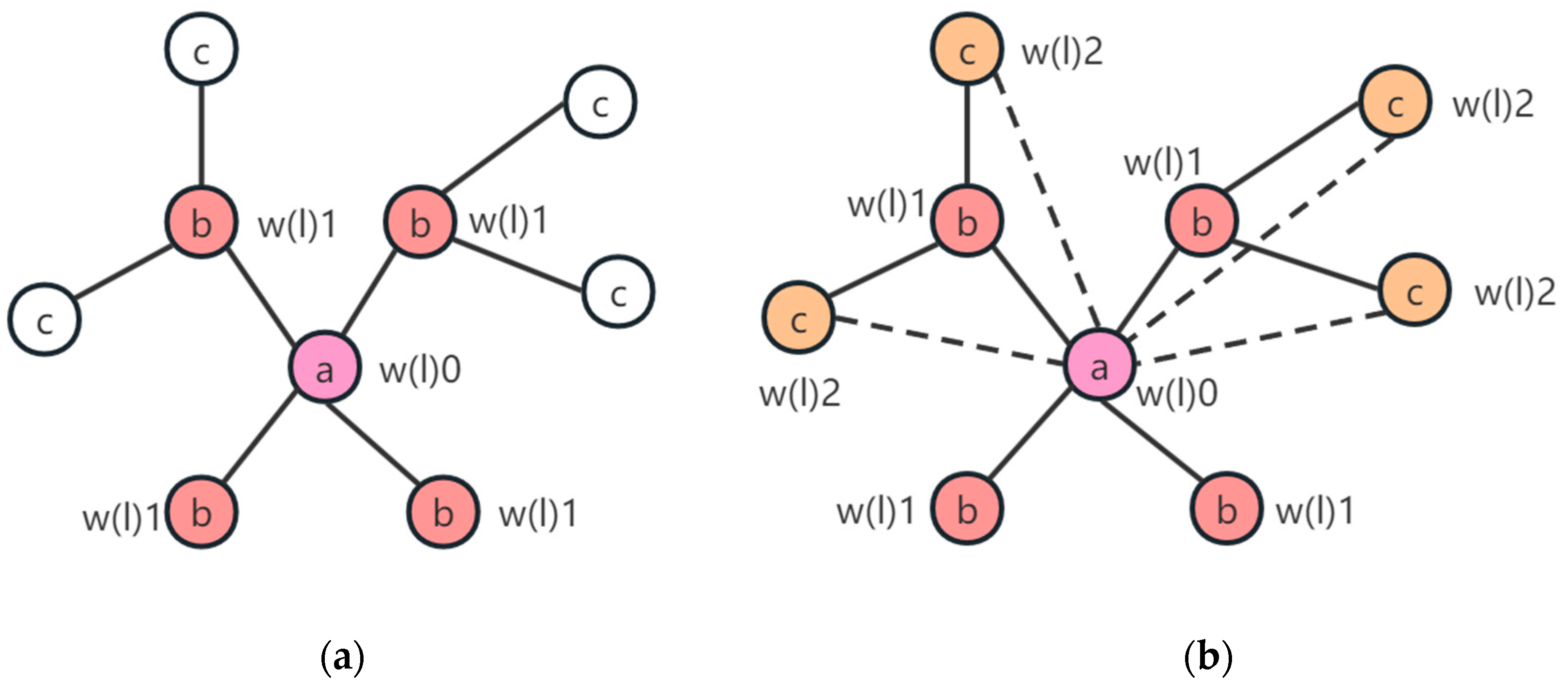
Figure 1a represents an example of OD flow, where inflow is the total number of people entering a region from other regions at a specific time, and outflow is the total number of people traveling from a region to other regions at a specified As shown in Figure 1b, the total OD flow in the central region is 9, with inflows and outflows of 5 and 4, respectively.

For historical data on crowd flow, the spatio-temporal dependence is complicated; the crowd flow of an area depends on its surrounding area, i.e., spatial dependence; and at a specific time, it depends on the relationship of crowd flow in the time period before and after it, i.e., temporal dependence.

Crowd flow prediction methods have been extensively studied. Traditional time-series prediction methods such as HA and ARIMA [2,3] have difficulty in capturing both temporal correlation and spatial dependence in historical data. Numerous deep learning models have arisen in the field of crowd flow prediction as a result of deep learning’s successful use in a number of fields. For instance, Zhang et al. [4] proposed ST-ResNet, predicting citywide crowd flows using deep spatio-temporal residual networks. Yao et al. [5] proposed a deep multi-view spatio-temporal network (DMVST-Net) based on a convolutional network (CNN) and a long- and short-term memory module (LSTM) for taxi demand prediction, which uses a CNN module to extract spatial correlation and an LSTM module to extract temporal dependence. Although the CNN method can extract features of the input data well, it can only be used for Euclidean data, i.e., regular spatial networks, which are not realistic and cannot model feature correlation at the same time.

Yu et al. [6] proposed a new deep learning framework combining graph convolution and 1D convolution to address the spatio-temporal data prediction problem in the traffic domain on the basis of spatio-temporal graph convolution (STGCN). Based on the previous study, Guo and Lin et al. [7] proposed an attention-based spatial-temporal graph convolutional network (ASTGCN) for traffic flow forecasting, which first inputs the traffic data into the attention mechanism to capture spatio-temporal relationships and then inputs them into the graph convolution structure to enhance the ability to model the dynamic spatio-temporal correlation of data. The model has a significant improvement in computational efficiency compared to the RNN model; however, these models share a common drawback. They train the model through static spatial graphs, ignoring the dynamic spatial changes of the crowd traffic network, and there is an obvious deficiency in the learning ability of spatial dependence.

Song et al. [8] argued that existing models typically use separate components to capture spatial and temporal correlations, and ignore the heterogeneity in spatio-temporal data. Therefore, they proposed to incorporate a synchronization mechanism based on previous studies and generated a new spatio-temporal synchronized graph convolutional network (STSGCN). Li and Zhu et al. [9] argued that the prioritized representation of a given spatial graph structure with imperfect adjacency connections may limit the effective spatio-temporal correlation learning of the model, the spatio-temporal fusion graph neural network (STFGNN), which can fuse different spatio-temporal graphs to improve the model prediction accuracy. Sun et al. [10] proposed the use of spatial graph convolution to create a multi-view graph convolution network (MVGCN) for the crowd flow problem by describing the crowd flow prediction in irregular regions as a spatio-temporal graph (STG) prediction problem, where each node represents a region with the time-varying flow. Xia et al. [11] proposed a three-dimensional graph convolution network (3D-DGCN) with point-of-interest (POIs) distribution as an additional feature, and used the K-mean algorithm to cluster N regions into K partitions for crowd flow prediction of irregular regions with POIs as features. Because similar functions in urban areas frequently have similar crowd flow patterns, similar functions are usually determined by similar POIs, which can significantly increase forecast accuracy [12]. Although urban area functions influence population flow patterns, POI features cannot adequately reflect urban area functions since they are inherently complex and dynamic. Although existing GCN methods have been used for crowd flow prediction with excellent results, they ignore the global spatial dependence. This is because it only focuses on the effect of direct neighboring nodes and ignores multi-order neighboring nodes [13]. Therefore, there is a deficiency in the model’s expressiveness due to interactions between the inflow and outflow of nodes. Moreover, there is a correlation between the flows in the adjacent time slots of the target node in the crowd flow data. A dense crowd flow at 9:00 a.m. in a location will affect the crowd flow at 10:00 a.m. because the flow in the previous time slice will correlate with the flow in the subsequent time slice.

In view of the above challenges and research implications, we propose a residual structure-based dynamic graph convolution model (Res-DGCN) on the basis of a deep understanding of crowd traffic data using the New York shared bicycle dataset and the New York yellow taxicab dataset, and improving the original model 3D-DGCN [11]. The following is a summary of this paper’s contributions:

• A new spatial attention module (SA) has been designed and integrated into the model. It obtains the dependencies between the current node and its indirect neighbors by learning the spatial correlations in the dynamic spatio-temporal graph in order to enable the coverage of the model by the indirect neighbors of the current node.
• In this paper, we propose an improved conditional convolution module (SCondConv), which can perform deep convolution to extract noise-uncorrelated features with high efficiency. This convolution layer extracts the trend of crowd flow within the neighboring time slices, filters the data noise, and enhances the correlation between the neighboring time slice data and the prediction results.
• Finally, the above modules are integrated with the dynamic graph convolution module to generate a traffic prediction model. Extensive experiments were run on two real datasets, and the results demonstrate that the model works better than existing baseline prediction methods.

The remainder of the paper is structured as follows. In Section 2, we introduce the current state of national and international research in the field of crowd flow prediction, as well as graph convolution and attention mechanisms. Section 3 gives a description of the prediction problem and the details of the model implementation. In Section 4, we introduce the data sources, and then analyze the experimental results and compare their performance with other baseline models. This paper is summarized in Section 5.

2. Methods

2.1. Graph Convolutional Network

Although urban area functions influence population flow patterns, POI features cannot adequately reflect urban area functions since they are inherently complex and dynamic. Despite the great success of CNNs in dealing with Euclidean data, researchers have recently attempted to apply CNNs to non-Euclidean data with mixed results. Right now, the most successful deep learning approach to solve this issue is graph convolutional.

Spectral and spatial methods are the two most popular strategies for graph convolution. The spectral method GCN is defined in the spectrum domain, and research into such methods were mostly based on [14]. After that, Defferrard et al. [15] proposed the ChebNet variant method, which represents a new stride in the development of GCNs and uses Chebyshev extensions to reduce the complexity of Laplace computation. Kipf et al. [16] transformed ChebNet into a simpler version that showed the best performance in various settings. Subsequently, Veličković et al. [17] introduced the attention mechanism into GCN and proposed the graph attention network (GAT), which achieves improved prediction accuracy by assigning different weights to neighboring nodes. The spatial approach’s goal is to map nodes in the sensory field to a fixed set, allowing convolution to be performed on various nodes with shared parameters. Niepert et al. [18] mapped nodes to a vector representation in which related nodes are placed similarly in space. However, GCNs are only weakly expressive since they do not consider neighboring nodes in the spatio-temporal graph.

2.2. Attentional Mechanisms

The attention mechanism is a popular neural network technique used in natural language processing, computer vision, and speech recognition.

The objective of the attention mechanism is to concentrate the incoming data on the information that is most pertinent to the subsequent processing step. The attention mechanism in neural networks is typically employed to choose input features or hidden states in order to efficiently complete various tasks. To enable the model to concentrate on the most relevant areas of the image and produce better descriptions, Xu et al. [19] presented two attention techniques. A graph neural network model based on attention mechanisms was proposed by Velickovic et al. [17] and employs a self-attentive mechanism to analyze graph structure data. In order to better understand the spatial and temporal information in geo-aware time series data, A multi-level attention network model for geo-aware time series prediction was put forth by Liang et al. [20]. This model uses multiple levels of attention mechanisms to capture various temporal dependencies.

We apply graph convolution and attention methods for modeling, accounting for the same high spatio-temporal correlation in crowd flow data, as inspired by the aforementioned.

3. Proposed Method

3.1. Problem Definition

The crowd flow problem is a typical time series prediction problem. In this study, we learn from the observation of historical crowd flow data to achieve the prediction of future crowd inflow and outflow at each node of the dynamic space-time graph (DSTG).

Definition: The DSTG is defined as an undirected graph $G=\left[V,A\right]$, $V$ is the set of nodes, $\left|V\right|=N$ is the number of nodes, which can be described as $V=\left\{v_i\right|i=\mathrm{1,2},3,\dots ,N\}$, $A$ denotes the dynamic adjacency matrix of nodes, $A_t\in R^{N\ast N}$. In any time interval $t$, the historical data can be described as $X_t\in R^{N\ast 2}$, where 2 is the inflow and outflow attributes.

Problem description: Let there be a graph $G=\left[V,A\right]$, and node history data ${\{X}_{t,i,j}\left|t=\mathrm{1,2},3,\dots ,t\right|i=\mathrm{1,2},3,\dots ,N|j=\mathrm{1,2},3,\dots ,N\}$, to forecast the result of the next step ${\{X}_{t+1,i,j}|i=\mathrm{1,2},3,\dots ,N|j=\mathrm{1,2},3,\dots ,N\}$, where $v_i\in V$ denotes an outflow node and _ $v_j\in V$ denotes an inflow node. The crowd flow prediction algorithm is formulated as function $Y=f\left(x\right)$, i.e.,

$${\widehat{X}}_{t+1,i,j}=f\left(X_{t,i,j}\left|t=\mathrm{1,2},3,\dots ,t\right|i=\mathrm{1,2},3,\dots ,N|j=\mathrm{1,2},3,\dots ,N\right)$$

(1)

In building the DSTG, this paper treats the historical OD flows as the edges of the DSTG, as shown on the left side of Figure 2a. The paper divides days into two categories: workdays and holidays, and divides each day into several time intervals. A spatio-temporal graph needs to be built for each time interval to form dynamic OD flows at different times. Afterwards, the average values of the OD flows obtained directly within the same time period for workdays and weekends are taken as the OD flow patterns X, respectively [11]. The normalized adjacency matrix at time interval t can be obtained with the following Equation (2):

$$A^t={\widehat{D}}^{-\frac{1}{2}}{X}_t{\widehat{D}}^{-\frac{1}{2}}$$

(2)

within it, ${\widehat{D}}^{i,i}={\sum }_j{X}_{t,i,j}$, we further add a self-loop to $A^t$, forming ${\widehat{A}}^t$, as shown in Equation (3):

$${\widehat{A}}^t=I+A^t$$

(3)

where $I$ is the identity matrix, $\widehat{A}\in R^{V\ast V}$ is the normalized adjacency matrix with self-loops at time interval t. Although the edges are for time intervals, the graph structure remains dynamic within each day, with a topology that changes over time. At the same time, we obtain the node attributes through the inflows and outflows $X_n$ within each time interval. Based on the above operations, the construction of the DSTG with dynamic graph structure and node attributes is completed.

3.2. Method Overview

The structure of the crowd flow prediction algorithm proposed in this paper is shown in Figure 2a. The algorithm can be decomposed into five steps: (1) spatio-temporal graph construction, where each node in the DSTG is represented by the OD flow of that node since the dependence between regions is changing dynamically over time; (2) feature modeling including spatio-temporal dependence on urban area crowd flow data and also point-of-interest (POI) and holiday information; (3) construction of dynamic graph convolutional layers, where the DSTG’s temporal and spatial characteristics are extracted using a continuous DGCN module, and a layer of convolutional layers is then added to scale the features and create output results with the required dimensions; (4) temporal correlation extraction, where in order to obtain the temporal correlation within consecutive time slices, we enhance the connection of neighboring time slices by aggregating the temporal features at the previous time slice of the prediction result through the SCondConv module; (5) model training, considering that the prediction structure is affected by the complex city-region function as well as the spatio-temporal dependence. To train both tasks at the same time, we employ the Huber loss function in conjunction with the cross-entropy loss function.

Among these five parts, three parts are improvements made based on the original model (3D-DGCN) (shown in the dashed boxes in Figure 2a), namely the SA module, SCondConv module, and loss function. They are further described in this section.

3.3. Spatial Attention Module

There may be some problems in using GCN alone to model the adjacency relationships between nodes in each irregular region (node). For instance, in a large city, there may be several indirect nodes between adjacent nodes, but the traditional GCN cannot capture the relationship between these indirect nodes. This paper proposes a spatial attention module (Figure 2b) to capture the spatial dependence of second-order and higher-order neighboring nodes, where the attention mechanism adaptively assigns different weight information to learn node spatial correlations, and the SA module improves the model’s ability to perceive spatial information.

Figure 3 is a schematic of node weight assignment. The multi-order surrounding nodes of the target node cannot be covered by graph convolution alone, but when used in combination with the spatial attention module, weights can be applied to the multi-order adjacent nodes to achieve coverage of the multi-order nearby nodes. The feature matrix $A\in R^{N\ast N\ast K}$ in Figure 2b was generated by fusing the crowd flow path matrix with POI features, which was obtained after node partitioning. The value of the matrix represents not only the correlation between two nodes, but also the strength of that correlation. Due to the certain discreteness of OD data, there are large differences in the influence factors between target nodes and different adjacent nodes. Therefore, it is first necessary to focus on key spatial features. Inspired by the above, SA firstly does the maximum and mean operations on the first dimension of the feature matrix, respectively, through which the mean and maximum values of each node on the dynamic changes of the human flow of the remaining N nodes (including its own node) can be obtained, which can make the model pay more attention to those neighboring nodes that are more relevant and important to the prediction results of the target node. Secondly, the two are combined to obtain the feature matrix after the focusing process and use it for the convolution operation. The reason for combining the two here is that the combination can generate connections that do not exist in the first place, and thus assign weights to the indirect neighbor nodes of the target node. In this paper, adaptive weight learning is performed through a convolution layer, which is the equivalent to using a convolution kernel for each node in the graph to extract the weights of nodes of order 0 to 3 centered on that node and rescaling the features by convolving the layer to produce a feature matrix of the specified dimension. The result is then added to the LeakyRelu activation function, which outputs non-zero values in the negative region and can retain the negatively correlated features in the feature matrix. Finally, a residual connection is applied, which enables the model to better learn the differences in the feature matrix before and after being processed by the SA module. The entire process can be summarized by Equation (4):

$${\widehat{A}}_t=LeakyRelu\left(f^{\mathrm{y}\ast \mathrm{y}}\left(\left[Max\left(A_t\right);Avg\left(A_t\right)\right]\right)\right)+A_t$$

(4)

where $A_t\in R^{N\ast N\ast K}$ represents the feature matrix, and $Max$ and $Avg$ denote the operations of taking the maximum and average values along the first dimension of the matrix, respectively. The function $f^{\mathrm{y}\ast \mathrm{y}}$ corresponds to a convolutional layer with a kernel size of y $\ast$ y, in this experiment, y is 9.

In the original model, the DGCN module captures the spatio-temporal dependencies between nodes, while the SA module enhances the node features for each time period to improve the model’s perception of multi-order neighboring nodes. Additionally, the spatial attention module helps the model handle spatial noise and irregularities present in the spatio-temporal graph, thereby further enhancing the model’s stability and robustness.

3.4. Improved Conditional Convolution Module

This paper proposes the SCondConv module, as shown in Figure 2c, which is an improvement upon the conditional convolution (CondConv) [21]. Since there is always a high similarity and correlation of OD data within neighboring time slices in the crowd flow prediction problem, the model needs to learn and exploit the contextual relationships between different locations and time steps in the spatio-temporal graph. Inspired by this, this paper captures the temporal dependence of crowd flow within neighboring time slices through the SCondConv module to enhance the correlation between the neighboring time slice data and the prediction results. The SCondConv module can dynamically adjust the size and shape of the convolutional kernel by inputting the content and contextual information of the spatio-temporal map so that the model has a more flexible perceptual field size to accommodate the extraction of feature requirements at different spatial locations and time steps, thus learning contextual relationships in the spatial and temporal information of neighboring time slices.

In order to alleviate the problem of gradient disappearance caused by the deepening of the network structure, the activation function Relu in the original CondConv module is replaced by Swish to generate a new conditional convolution module in this paper. Swish is not only nonlinear but also has a smoother curve near zero, which helps alleviate the issue of gradient vanishing. Additionally, the Swish function exhibits a certain level of saturation, which can help mitigate the overfitting of the model. The Swish activation function is defined by Equation (5):

$$Swis\mathrm{h}\left(x\right)=x\cdot Sigmoid\left(x\right)$$

(5)

The execution process of the SCondConv module, as described in Equation (6):

$$SCondConv\left(X_t\right)=Swish\left(\left({\alpha }_1{W}_1+\dots +{\alpha }_n{W}_n\right)\ast X_t\right)$$

(6)

where $X_t\in R^{B\ast C\ast 1\ast N}$ represents the crowd flow data at time t, and each ${\alpha }_i=r_i\left(x\right)$ is a scalar weight associated with the sample, learned through gradient descent. Each convolutional kernel $W_i$ has the same dimensions as regular convolution parameters. The variable $n$ represents the number of experts, and $Swish$ corresponds to the activation function defined in Equation (5).

The weighted parameters ${\alpha }_i=r_i\left(x\right)$, learned through backpropagation, exhibit data dependency. They allow the module to obtain different input functions based on different input samples. These parameters are obtained through Equation (7):

$$r_i\left(x\right)=Sigmoid\left(GAP\left(x\right)R\right)$$

(7)

where R represents the weight mapping matrix that combines the inputs to the n experts.

In the context of predicting crowd flow in urban areas, most existing studies [8,22,23] grid the urban regions, transforming the time series data into a spatio-temporal graph structure to be trained by graph convolutional models. However, due to the limitations of convolutional kernels, each layer’s ability to extract spatio-temporal correlations is often limited. Moreover, when the network structure of the model is deeper, the deeper layers are more prone to gradient disappearance and gradient explosion during training, resulting in poor convergence [24]. To address this challenge, He et al. [25] proposed a residual neural network. Therefore, this paper proposes a deeper network architecture to extract features from the spatio-temporal graph and incorporates residual connections into the network. As shown in Figure 2a, the model’s prediction results are connected with the SCondConv results using a residual connection.

First of all, while the ScondConv module can learn contextual relationships, it can also reduce the number of parameters of the model by sharing parameters, which can speed up the training and inference of the model and make it more practical in real life. Secondly, because the ScondConv module can adjust the weights of the convolution kernel according to the trend of human traffic within the neighboring time slices, placing the ScondConv module in the place of the residual connection can make the model better capture the time dependence and thus improve the modeling ability for the time series.

3.5. Loss Function

To facilitate the training of the model, this paper combines prediction training with region segmentation training to achieve better solutions. We shall introduce the two tasks successively in this section.

Prediction Training Task. Since the SA module and ScondConv module are added to the original model in this paper, it increases the complexity of the model, which will lead to overfitting. Secondly, the analysis of the dataset used for this experiment using the 3-Sigma criterion shows (see Section 4.1) that there are a large number of outliers in it. Therefore, in this paper, Huber loss is chosen as the loss function to replace the mean square error (MSE) loss function used in the original model, which outperforms the MSE loss function in both problems mentioned above. The Huber loss function has the following advantages: (1) Strong Robustness: Compared to the Mean Squared Error (MSE) function, the Huber loss is less sensitive to outliers. It can better adapt to data with a higher presence of noise or outliers. (2) Continuously Differentiable: The Huber loss is continuously differentiable for the majority of points, which allows it to be used in conjunction with other continuously differentiable optimization methods such as backpropagation and the Adam optimizer. This facilitates the process of solving model parameters. (3) Parameter Control: During the parameter estimation process, the Huber loss can balance the convergence speed and robustness to outliers through the parameter α. Compared to more traditional approaches for handling outliers, it provides a better balance. Equation (8) depicts the loss function for the prediction task:

$$L_{Huber}\left(Y,\widehat{Y}\right)=\left\{\begin{array}{c}\frac{1}{2}{(Y-\widehat{Y})}^2,\left|Y-\widehat{Y}\right|\le \alpha \\ \alpha \left|Y-\widehat{Y}\right|-\frac{1}{2}{\alpha }^2,\left|Y-\widehat{Y}\right|>\alpha \end{array}\right.$$

(8)

where $Y$ represents the historical ground truth data, $\widehat{Y}$ denotes the model’s predicted results, and $\alpha$ is the hyperparameter that controls the range of the mean squared error loss.

For the region segmentation training task, the city region network graph divides different areas in the city into irregular regions based on the city road network. Each region may have different functions in the city, such as residential or commercial areas. Different regions exhibit similar temporal trends during the same time intervals on workdays or holidays. Therefore, using the traffic road network to perform irregular segmentation of regions is more suitable for data analysis and learning spatial-temporal correlations.

To solve the aforementioned issues, Xia et al. [11] proposed a method in which nodes are partitioned into separate subsets, and different parameter weights are assigned to each partition. The number of partitions is fixed, while the number of nodes within each partition varies. They utilized POI (Point of Interest) data to aggregate the attributes of each region, transforming nodes into regions with POI attributes. The original model used K-means clustering to group the POI features $f$ of $N$ regions into K partitions. The partition of region $v_i$ is represented as $\left\{{\mathsf{\Omega }}_i\right|i=\mathrm{1,2},3,\dots ,K\}$. Spatial GCN layers were employed for node partitioning, with node features $F\in R^{N\ast \left|C\right|}$ as the input. The expression for the output Z is given by Equation (9):

$$Z=Softmax\left(\stackrel{-}{A}\sigma \left(\stackrel{-}{A}F{W}_{\left(1\right)}^s\right)W_{\left(2\right)}^s\right)$$

(9)

where $W_{\left(1\right)}^s\in R^{\left|C\right|\ast C^{\prime }}$ and $W_{\left(2\right)}^s\in R^{C^{\prime }\ast K}$ are the parameters for each layer, where $C^{\prime }$ represents the number of channels in the hidden layer. Since the GCN model in this study does not consider the temporal relationship of the data, the average of ${\widehat{A}}_t$ is used as the adjacency matrix. The average is computed as $\stackrel{-}{A}=\frac{1}{T}\sum _{t=0}^T{\widehat{A}}_t$, where ${\widehat{A}}_t$ is the normalized adjacency matrix with self-loops at time t, and T is the total number of time slices in the dataset. Based on the partitioning scheme, the original model calculates the adjacency matrix $A_k^{i,j}$ for the GCN used in prediction, as shown in Equation (10):

$$A_k^{i,j}=A^{i,j}·Z^{j,k}$$

(10)

By merging the region attributes based on the POI features, we obtain the adjacency matrix $A_k^{i,j}$ that captures the similar patterns of city functionalities, taking into account the impact of complex urban functional structures on population flow. This adjacency matrix is derived using Equations (9) and (10), and it enables the model to achieve better performance by considering the influence of urban functional structures on population movement. Equation (11) illustrates how the original model uses the cross-entropy loss on labeled nodes as the loss function for semi-supervised learning:

$$L_s=-\sum _{v_i\in V_L}\frac{\ln \left(Z^{i,{\varphi }_i}\right)}{\left|V_L^{{\varphi }_i}\right|}$$

(11)

where ${\varphi }_i\in \{1,\dots ,K\}$ represents the partition of node $v_i$, $V_L$ is the set of all labeled nodes, and the subset $V_L^{{\varphi }_i}$ contains all labeled nodes within partition ${\varphi }_i$. Since the sizes of each partition are not uniform, the term $\frac{1}{2}\left|V_L^{{\varphi }_i}\right|$ is used as a normalization factor.

We combined the above two training tasks and defined a multi-task learning loss function as in Equation (12):

$$L=L_{Huber}+\beta L_s$$

(12)

where the Huber loss function, which calculates the model’s error in predicting node flow, is represented by the first term $L_{Huber}$. The cross-entropy loss function for semi-supervised node classification is the second term, $L_s$, which the error of the model in predicting node flow categories. $\beta$ is the weight that balances these two loss functions. The model is adjusted to produce reliable output results by taking advantage of the association between population flow patterns and urban area structure.

The Huber loss function Is suitable for regression problems, while the cross-entropy loss function is commonly used for classification problems. In the task of predicting population flow, the flow of nodes is typically influenced by various factors such as weather, time, and geographic location. These factors can result in complex variations in node flow, making it challenging to accurately capture them using a single loss function. By incorporating both the Huber loss and the cross-entropy loss, the model can take into account the diverse nature of node flow changes more comprehensively. This enables more accurate prediction of population flow, enhancing the model’s performance and robustness in handling the complexities of the task.

4. Experiments and Analysis

4.1. Datasets

In this experiment, all the data used are real-world datasets. To evaluate the performance of the model, the study conducted validation on two datasets: TaxiNYC and BikeNYC.

TaxiNYC dataset consists of taxi trip records in New York City, provided by the New York City Taxi and Limousine Commission. The experiment used a subset of the dataset from 1 July 2017 to 30 September 2017. It includes detailed information such as the pickup time and location, drop-off time and location, fare, passenger count, payment method, and more for each taxi trip.

BikeNYC dataset is an open dataset provided by the NYC Transportation Department, containing data from a bike-sharing system. The experiment used a subset of the dataset from 1 October 2014 to 31 December 2014. The dataset includes information such as the start time, start and end locations, trip duration, distance, user type, and additional derived data such as latitude and longitude of each station, station names, capacity, and usage information.

Since both datasets are collected in New York City, it is possible to use the same irregular spatial partitioning and Points of Interest (POI) [11] for both datasets. The total number of irregular partitions in this case is 82. As shown in Figure 4, the 82 irregular partitioned areas of New York City are illustrated.

We mapped the mobility data from both datasets to the irregular regions representing the crowd movement. The sampling interval was set to 1 h, resulting in OD (Origin-Destination) flow as shown in Figure 1. There were a total of 26,202 Points of Interest (POIs) categorized into 9 types: Food, Residential, Shop and Service, University, Nightlife, Tourist and Transport, Arts and Entertainment, Professional Places, and Outdoor & Recreation.

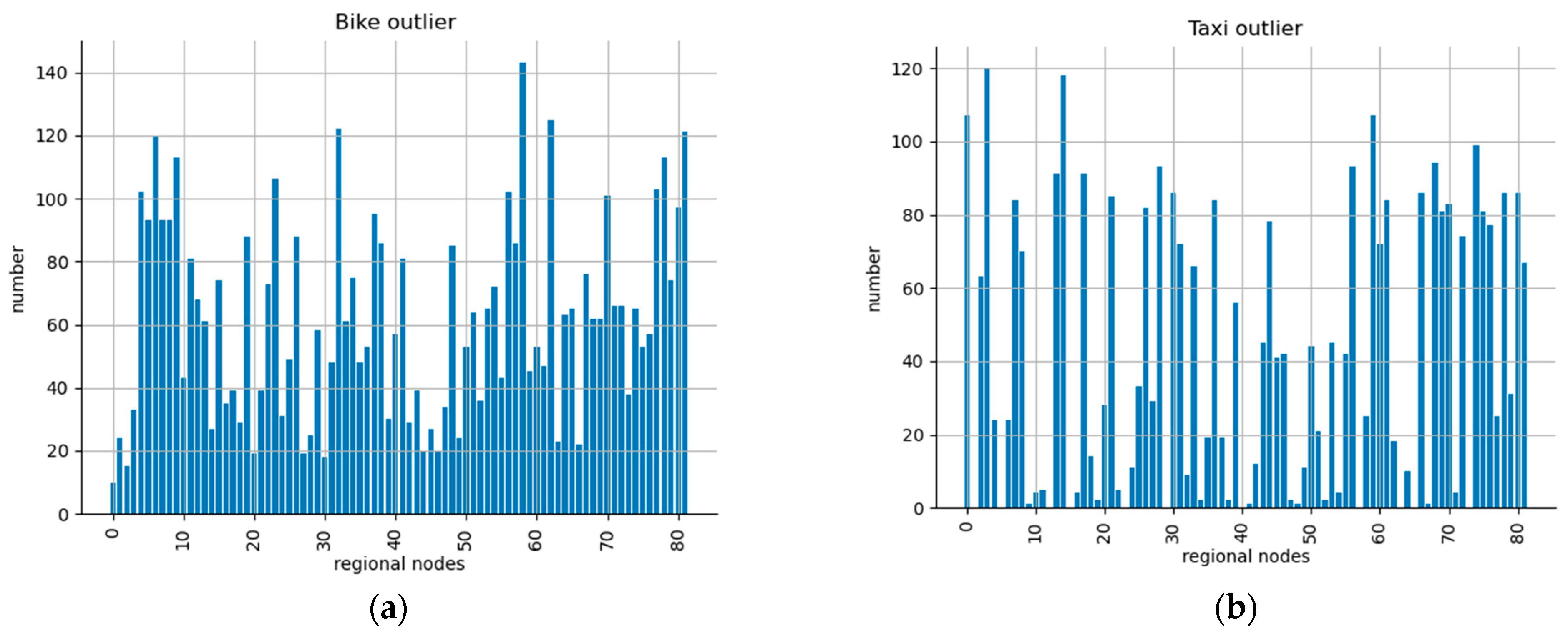
Detecting and handling outliers is crucial to improve the quality and reliability of crowd flow data and reduce errors and uncertainties caused by outliers, thus providing better support for relevant decisions. In this study, we employed the 3-Sigma criterion to detect outliers in both datasets. According to the 3-Sigma criterion, a data point is considered an outlier if its value exceeds the mean plus or minus three times the standard deviation. The experimental results are presented in Figure 5a,b, showing the presence of outliers in both datasets. There are noticeable deviations from the average value in OD flow during certain periods such as severe weather conditions or weekends and holidays. For example, during severe weather, people tend to take taxis instead of walking or cycling, while on weekends and holidays, people prefer to ride bicycles or walk instead of taking taxis.

4.2. Experimental Environment and Parameter Settings

The NVIDIA Tesla T4 graphics card was used for the experiments in this study.

To assess the effectiveness of the experimental models, we followed the commonly used methods in the field of crowd flow prediction. The Root Mean Square Error (RMSE) and Mean Absolute Error (MAE) were adopted to assess the errors between the predicted values and the ground truth values. The equations for RMSE and MAE are shown in Equations (13) and (14), respectively:

$$RMSE=\sqrt{\frac{1}{n}\sum _{i=0}^n{(Y_i-\widehat{Y_i})}^2}$$

(13)

$$MAE=\frac{1}{n}\sum _{i=0}^n{|Y}_i-\widehat{Y_i}|$$

(14)

where $n$ is the number of samples, $Y_i$ is the ground truth value, and $\widehat{Y_i}$ is the predicted result of the model:

Based on the grid search method, the optimal parameters for crowd flow prediction using Res-DGCN are determined and presented in

Table 1. Model parameter settings.

Parameter	TaxiNYC	BikeNYC
Number of historical time intervals	5	5
Loss function weights β	5	70
Huber function parameter α	15	30
Number of DGCN layers	4	4

.

The historical time interval of 5 indicates that the model uses the past five hours of historical data to predict the result for the next hour, which is a single-step prediction. For instance, to predict the crowd flow data at time step 5, the input consists of the crowd flow data at time steps 0, 1, 2, 3, and 4. For the experiment, the dataset is split into three sections: the training set, validation set, and test set, with corresponding temporal fractions of 80%, 10%, and 10%.

4.3. Baseline Methods and Comparative Experiments

To assess the practical performance of Res-DGCN, we compared it with traditional time series forecasting methods as well as some excellent graph convolutional networks.

• HA [4]: This model refers to the Historical Average model, which predicts based on the historical average values.
• ARIMA [26]: This model refers to the AutoRegressive Integrated Moving Average model, which is a forecasting model based on time series analysis.
• STGCN [13]: This model is a neural network model based on spatio-temporal graph convolutions. It solely relies on historical inflow and outflow data for prediction and does not take into account OD flow and POI data.
• DCRNN [27]: This model is based on a combination of recurrent neural networks and diffusion convolutional neural networks. Similar to STGCN, it only utilizes historical crowd flow data for prediction.
• STGNN [28]: This model is another type of network model based on spatio-temporal graph convolutions. Unlike STGCN with gated convolutions, STGNN utilizes GRU and Transformer to capture short-term and global temporal dependencies for prediction.
• MVGCN [10]: This model is a crowd flow prediction model based on multi-view graph convolutional neural networks. Unlike traditional single-view graph convolutional neural networks, MVGCN utilizes multiple views of spatio-temporal data to improve prediction accuracy.
• 3D-DGCN [11]: This model is a crowd flow prediction model based on three-dimensional graph convolutional neural networks. It serves as the baseline model for the proposed model in this paper.

The results of the comparative experiments in this paper are presented in

Table 2. Model performance comparison.

	BikeNYC		TaxiNYC		Training Time/s	Number of Parameters
	MAE	RMSE	MAE	RMSE
HA [4]	9.97	17.05	47.33	88.98	0	0
ARIMA [26]	10.41	19.14	46.78	85.25	0	0
STGCN [13]	6.49	11.73	42.58	75.47	272	454,000
DCRNN [27]	5.88	9.85	39.64	67.57	10756	372,353
STGNN [28]	5.79	9.80	37.30	65.12	2995	617,985
MVGCN [10]	5.65	9.64	-	-	-	-
3D-DGCN [11]	4.81	7.76	33.06	60.23	3130	145,677
Res-DGCN	4.55	7.38	29.93	54.92	6321	149,867
Δ	5.2%	4.8%	9.4%	8.8%	-	-

and

Table 3. Results of ablation experiments.

SA	sCondConv	Huber	BikeNYC		TaxiNYC
			RMSE	Δ	RMSE	Δ
-	-	-	7.76	0	60.23	0
√	-	-	7.64	1.5%	56.4	6%
-	√	-	7.52	3%	58.11	3.5%
-	-	√	7.68	1%	58.3	3.2%
√	√	-	7.58	2.3%	57.93	3.8%
√	-	√	7.58	2.3%	55.76	7.4%
-	√	√	7.43	4.2%	56.51	6.1%
√	√	√	7.38	4.8%	54.92	9.4%

. In these tables, Δ represents the percentage improvement in performance compared to the 3D-DGCN model.

Table 2 shows that Res-DGCN performs better than the baseline methods and obtains the best results on both datasets. Traditional time series analysis methods exhibit lower predictive accuracy as they can only handle simple time series data and are unable to capture complex patterns and non-linear trends in time series, making it challenging to deal with the complex variations and noise interference in real-world applications. The deep learning-based methods, however, exhibit substantial advancements as they are all founded on graph neural networks for crowd flow prediction. What they have in common is that they all use graph neural networks to model spatial relationships and temporal relationships. In terms of the computational complexity of the model, Res-DGCN has a deeper network structure compared to 3D-DCGN, so the training time of the model becomes longer, but there is a greater improvement in prediction accuracy. Compared with the remaining baseline models, Res-DGCN has a greater advantage in terms of the number of parameters, which indicates that the model is feasible to be deployed in practical program applications.

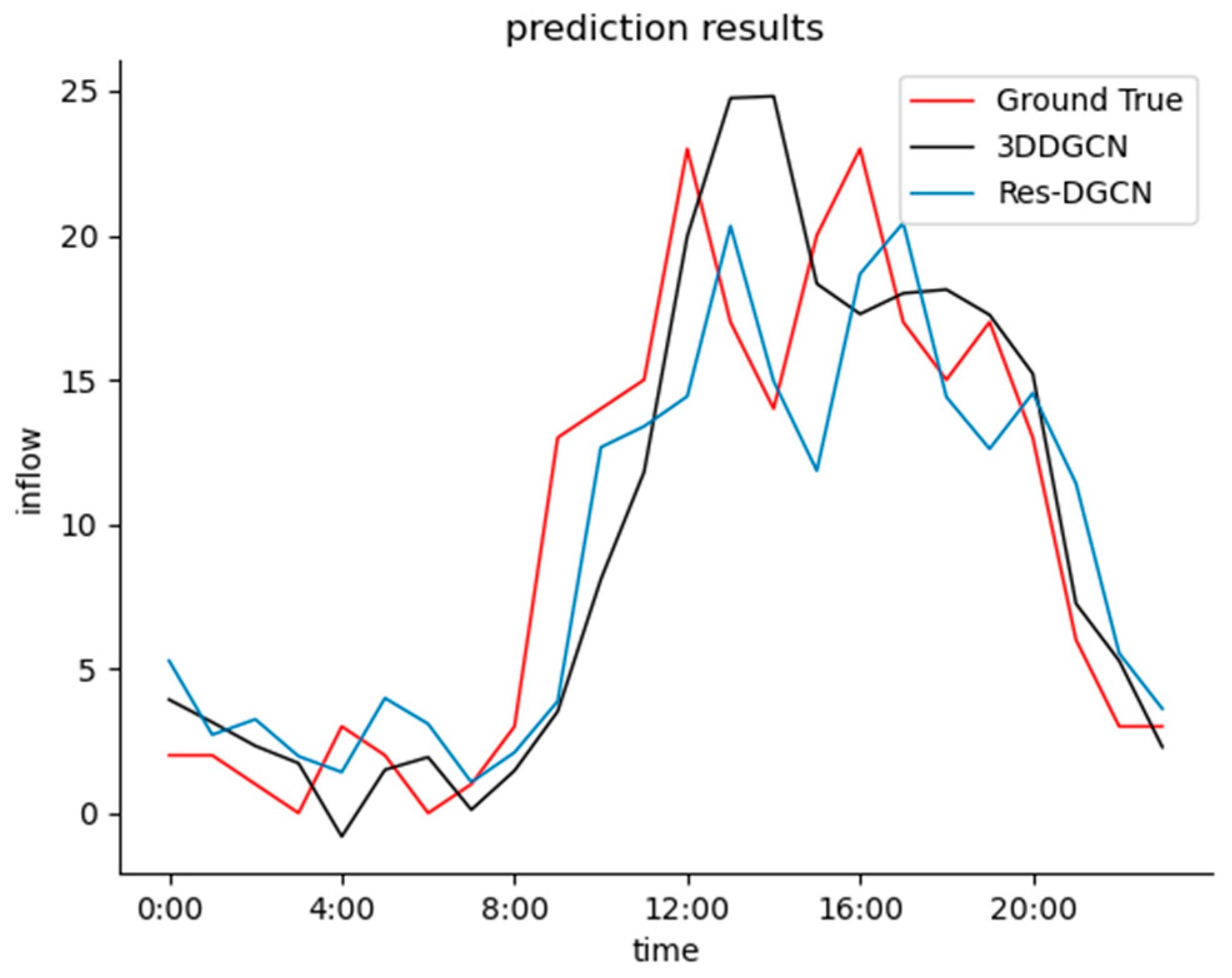
The comparison between our model’s predicted values and the historical ground truth data is shown in Figure 6. It is clear from the graph that our model is sensitive to changes in the historical data. Although the predicted curve lags behind the true values to some extent, it effectively fits the true value curve in a timely manner. The predicted results of our model are closer to the historical ground truth values compared to the 3D-DGCN model. During the time points of 12:00 and 16:00, the real data exhibit peak periods corresponding to commuting hours, but the predicted curve of the 3D-DGCN model fails to capture this characteristic and does not show significant upward and downward trends. In contrast, the performance of Res-DGCN is better. This is because the proposed conditional convolutional module in this paper can effectively learn the temporal correlations among neighboring time steps. It can dynamically generate convolutional kernels based on the input conditions, enabling the model to adaptively learn feature representations under different input conditions.

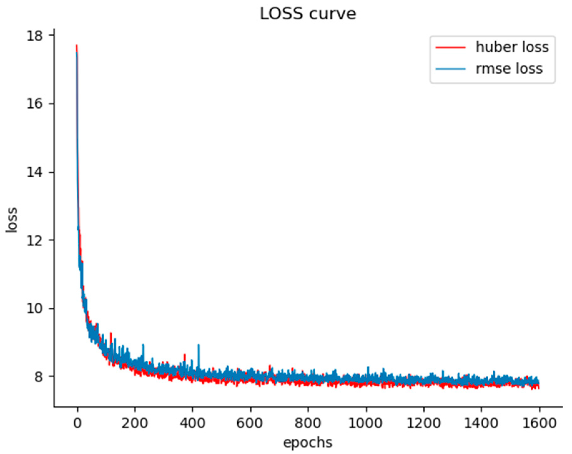
Figure 7 shows the loss curves of two loss functions generated during the training of the BikeNYC dataset. It depicts a comparison of our model’s Huber loss function and RMSE loss function’s loss variation. It is evident that the Huber loss function achieves the lowest and most stable loss curve. In terms of the obtained loss values, the Huber loss function outperforms the RMSE loss function in terms of model performance.

4.4. Ablation Experiments

This section performs ablation experiments to assess each component’s impact on the model’s accuracy in order to show the effectiveness of the components designed in this paper. The component units used in the experiments include SA, sCondConv, and Huber. By combining these units in different ways, six variants of Res-DGCN are designed to understand the roles and contributions of each component in the model, providing guidance for further optimization of the model.

As shown in Table 3 (Δ indicates percentage of performance improvement), the three components proposed in this paper have significantly enhanced the model’s prediction accuracy. Removing any of these components would increase the prediction error. In the TaxiNYC dataset, considering the spatial dependency between the target node and multi-order neighboring nodes appears to be more important, indicating the crucial role of the SA module. On the other hand, in the BikeNYC dataset, considering the temporal trend of nearby time steps seems to be more important, highlighting the significance of the sCondConv module. Since the proposed model needs to simultaneously consider both spatial and temporal information along with input features, the SA module and sCondConv are used in combination.

However, in this ablation experiment, the SA+sCondConv variant showed a 2.2% decrease in prediction accuracy compared to the SA variant in the Taxi dataset. Similarly, in the Bike dataset, the SA+sCondConv variant showed a 0.7% decrease in prediction accuracy compared to the sCondConv variant. However, in the complete Res-DGCN model, the prediction accuracy improved by 1.8% to 6.2% compared to the single-module variants. The experiment demonstrates that the Huber loss function can reduce the model’s sensitivity to outliers, leading to improved prediction accuracy. Whether used alone or in combination, the Huber loss function contributes to varying degrees of enhancement in the model’s accuracy.

5. Conclusions

This paper proposes a novel Dynamic Graph Convolutional Network (Res-DGCN) based on residual structures for predicting the inflow and outflow of populations in irregular urban areas. The model combines spatial attention mechanism and spatio-temporal convolution including graph convolution in the spatial dimension and conditional convolution in the temporal dimension to effectively capture the spatio-temporal correlations in population flow data. Extensive experiments were run on two real-world datasets, and the outcomes show that the proposed model performs better than the baseline models. Our model is a general model from the perspective of traffic prediction. In this paper, we propose the spatial attention module, which can extract multi-order neighbor node features and can be applied to the fields of visual detection and image segmentation. The improved conditional convolution module can capture the connection of proximity time slices with downward perception capability, which can be extended to apply to image super-resolution and natural language processing fields. Res-DGCN also has the limitation that it requires crowd flow data to have both temporal and latitudinal information of origin and destination, two features that cannot be easily transferred to other tasks dealing with spatio-temporal data. Currently, the work in this paper focuses on single-step crowd flow prediction. In future work, we will consider implementing multi-step prediction and studying the heterogeneity of crowd flow data to make the prediction model more interpretable, and we plan to combine the Res-DGCN model with other deep learning methods to better learn the spatio-temporal features hidden in the crowd flow data.