Risk Propagation Mechanism and Prediction Model for the Highway Merging Area

Abstract

The merging area is one of the most accident-prone areas on highways. After an accident occurs, the risk will propagate along the main road over a certain range and time. Therefore, the study of the propagation mechanism of accident risk will help to quantify the driving risk in this region. An effective risk prediction model is important for improving traffic control measures in this specific area. In this study, simulation experiments were conducted in SUMO (Simulation of Urban Mobility) to obtain the accident and risk propagation data in merging areas. Firstly, the Gaussian plume model was optimized for the merging area situation to determine and divide the impact range of the accidents. Then, different accident scenarios in the merging area and downstream were simulated with different input flow rates to study the time and speed of risk propagation in the three-level affected areas. Finally, LSTM (long short-term memory) and RNN (recurrent neural network) models were built to predict the accident risk in the merging area. The results showed that the LSTM model had higher accuracy. This study provides an innovative insight into the propagation process of merging area accidents. It is of benefit to the development of post-accident control measures.

1. Introduction

The merging area is a black spot for traffic accidents due to conflicts between merging vehicles and mainline vehicles. However, the impact of traffic accidents is not a static factor. Their risks can affect other system elements in space and time. Therefore, when analyzing traffic accidents, it is necessary to study the interactions between various elements and their impact on the mechanism of risk propagation.

1.1. Mechanism of Traffic Accident Risk Propagation

Past research has mainly focused on analyzing the queuing phenomenon that occurs after an accident and assessing the level of impact on the surrounding road network. Michalopoulos [1] established a method to simulate traffic flow density variation using fluid mechanics. This method considered traffic flow fluctuations as waves in water and studied the propagation characteristics of traffic waves during the congestion–dispersion process in traffic jams. Sheu et al. [2] calculated accident delay value, vehicle queue length, and congestion duration based on arrival–departure curves using a queuing model for congested vehicles on highways. However, the model could not predict real-time traffic states. Deo et al. [3] considered various factors such as incident location, queue length, weather conditions, and lane closures. They established a survival model based on severity parameters to estimate the duration of the event and its impact. Lawson et al. [4] improved the cumulative arrival–departure graph by describing the number of queued vehicles as a function of time. They determined the impact range of upstream congestion on bottleneck sections. However, the model was only suitable for studying unsaturated situations. R. Smid [5] provided a spatial impact calculation method for highway accidents based on basic traffic flow analysis principles. The method considered the imbalance between traffic demand and supply as the cause of traffic accidents. Khattak et al. [6] predicted the duration of accidents on highways using an integrated accident online management tool based on rigorous statistics and queuing models.

Chung et al. [7] used the BIP algorithm to quantify the delay caused by highway accidents. They identified factors that caused such delays by predicting the reliability of random accident events with circular detectors. Zhang et al. [8] proposed a prediction method for the spatial impact propagation of traffic events on highways. They improved the application method of the traditional traffic flow fluctuation theory by quantifying the traffic flow operation characteristics. Hu et al. [9] developed a method for predicting the range of accident impact by determining the traffic flow redistribution on surrounding diversion routes. They used the inverse calculation of the OD matrix and estimated the total travel time under induced conditions to provide guidance for traffic diversion measures. Li et al. [10] established a prediction model for the impact range of sudden events by using the index of the variation index and deviation of the total travel time of vehicles in the region as a criterion. Yu et al. [11] calculated the traffic wave speed and queue length to study the diffusion range of traffic accidents in different time periods. Li et al. [12] established an estimate model for the radiation range of traffic flow under accident conditions based on TransModeler simulation. Ma [13] constructed a staged model to predict the duration of highway traffic accidents. They extensively used historical traffic data to predict the time of accident reporting and handling. Lin et al. [14] predicted the scope of accident impact based on the delay time of the accident-generated queue length and the recovery time of the queue length. They proposed several post-accident traffic organization measures. Jin et al. [15] quantitatively determined the accident impact area in three levels (point, line, and surface) based on maintenance requirements, traffic flow theory, and travel times.

The above studies show that various approaches and models have been employed to analyze the effects of traffic accidents and predict their duration and spatial impact. These methods include simulating traffic flow density variations using fluid mechanics, queuing models for congested vehicles on highways, survival models based on severity parameters, and spatial impact calculation methods. Additionally, predictive techniques based on statistical analysis, queuing models, traffic flow theory, and historical data have been proposed. These studies have contributed to understanding queuing behavior and the impact of accidents on traffic. However, these models and methods have certain limitations and areas for improvement, such as poor data quality and difficulty in determining critical parameters at the microscopic level.

1.2. Study on Traffic Accident Risk Prediction

Generally, predicting the risk of traffic accidents requires a large amount of traffic flow data. By mining and extracting the characteristics of traffic accidents and establishing prediction models, it is possible to predict traffic accident risks in a certain area over a period. Traditional methods usually adopt parameter modeling methods. For example, Hossain et al. [16] comprehensively used a random multinomial logit model and Bayesian belief network to predict the risks of highway traffic accidents in real time. Zhai et al. [17] used the Bayesian logistic model to predict the risks of highway traffic accidents under heavy fog conditions. Sun et al. [18] proposed an accident probability prediction model based on a dynamic Bayesian network using speed-time series data. In recent years, some researchers have also built some non-parametric machine learning models [19]. For example, Yang et al. [20] explored the application of support vector machines in the real-time risk division of traffic flow. Zhang et al. [21] proposed a real-time traffic accident prediction method based on the AdaBoost classifier by selecting the standard deviation features of traffic flow characteristics. Qu et al. [22] used support vector machines to evaluate the risks of rear-end accidents on highways. Fu et al. [23] constructed a highway accident risk model based on the random forest algorithm. With the continuous development of deep learning technology, many researchers have also applied deep neural network models in the field of risk assessment. Zhou et al. [24] constructed a model based on a differential time-varying graph convolutional network and used multi-task learning methods to predict both traffic flow and accident risks. Yuan et al. [25] proposed the Hetero-Conv LSTM model, which collected multi-source heterogeneous data to predict the number of traffic accidents occurring in the next time step. Yu et al. [26] constructed a traffic accident prediction model based on a deep spatiotemporal graph convolutional network based on traffic flow speed, weather conditions, and POI (point of interest) hotspots. Ren et al. [27] used traffic flow, weather, and air data to predict the trend of regional traffic accidents through the LSTM model. Their approach showed significant improvements compared with SAE (sparse autoencoder) and SVM (support vector machine) models. Chen et al. [28] established a stacked autoencoder model to study the impact of pedestrian flow on traffic accident risks.

The above studies have identified the applications of traffic flow data and historical accident data in real-time accident risk prediction. However, most of these studies focused on ordinary sections of highways and urban roads. Most of these results neglected the spatial characteristics of accidents and the impact of potential factors on accidents.

1.3. Summary

Many past studies have focused on the macroscopic factors affecting accident risk propagation and utilized machine learning methods for prediction. However, these studies also faced significant challenges such as poor data quality and difficulty in determining critical parameters at the microscopic level. In this study, we aimed to address some of these limitations by utilizing a simulation approach to investigate risk propagation patterns in highway merging areas. Specifically, our research includes building a detailed simulation dataset and improving the Gaussian plume model for microscopic accident risk prediction in such areas. The contribution of our study is the consideration of both macroscopic and microscopic factors when investigating accident risk propagation patterns. Through our proposed model, the complex mechanism of such phenomenon can be better understood. The detailed simulation dataset and an improved Gaussian plume model were built for the microscopic accident risk prediction in such areas.

The rest of this paper is organized as follows. Section 2 proposes the concept of accident risk propagation in merging areas and defines the regional risk index. Section 3 establishes a Gaussian plume model of the accident impact, which classifies the accident’s impact range. Section 4 studies the accident impact propagation mechanism in merging areas through simulation experiments. Section 5 builds and compares two traffic accident risk prediction models for merging areas. Finally, Section 6 concludes the contribution of this paper and future work for this research.

2. Concept of Accident Risk Propagation

The merging area of highways is a high-risk area due to the interaction between main road vehicles and ramp vehicles. When a traffic accident occurs, rapid changes in traffic speed and competition for right-of-way among vehicles will change the risk level of upstream sections. Additionally, the driver’s non-standard operations, unsuitable road design, and traffic environment interference also increase the accident risks. These risks will accumulate along the traffic flow and spread through congestion and dissipation waves, as shown in Figure 1. After an accident occurs, the following vehicles need to brake to avoid colliding with the accident vehicles. At the same time, the vehicles on the fast lane will also be affected by the lane-changing behavior of the vehicles on the ramp. Therefore, the closer the vehicle is to the accident site, the more likely it is to be affected. Its driving risk increases accordingly. The farther the vehicle is from the accident site, the less affected it is. If the vehicle is far enough away, its driving risk will almost be unchanged.

However, risk propagation is a dynamic process, as shown in Figure 2. In the early stage of an accident, the risk of collision increases due to the high likelihood of secondary accidents caused by the sudden braking of vehicles. After a period, the traffic flow near the accident position gradually slows down, and the risk between vehicles decreases. At the same time, the risk caused by sudden brakes propagates to the upstream of the traffic flow, resulting in high risk in the upstream area. The collision risk within the traffic flow dissipates when the traffic flow stabilizes.

2.1. Risk Indicators

Time-to-collision (TTC) is used to evaluate the potential collision risk between two vehicles. It is defined as the time it takes for two vehicles to collide if they continue to move in their current direction at their current speed. The equation of this index is as follows:

$$TT{C}_i(t)=\frac{S}{V}=\frac{x_{i-1}(t)-x_i(t)-l_{i-1}}{v_i(t)-v_{i-1}(t)}$$

(1)

where $TT{C}_i(t)$ represents the time-to-collision between vehicle $i$ and the preceding vehicle, where $t$ is the time at which the distance between vehicle $i$ and vehicle $i-1$ will become 0. $S$ represents the headway distance between vehicle $i-1$ and vehicle $i$; $V$ represents the relative velocity between vehicle $i-1$ and vehicle $i$; $x_i(t)$ and $x_{i-1}(t)$ are the head positions of vehicle $i$ and vehicle $i-1$, respectively; $v_i(t)$ and $v_{i-1}(t)$ are the instantaneous velocities of vehicle $i$ and vehicle $i-1$, respectively; and $l_{i-1}$ is the length of the preceding vehicle $i-1$.

2.2. Accident Severity Assessment

To define the accident severity, a threshold needs to be determined. Currently, most studies use the cumulative frequency curve method to determine the threshold. Here, the 15% and 85% percentile values of the TTC cumulative frequency curve were chosen as the thresholds for severe and general accidents. According to previous research [29], the threshold for severe accidents is usually between 1.5 and 4 s, while the threshold for general accidents is between 3 and 8 s. Therefore, severe accidents are defined as TTC < 3 s, general accidents are defined as 3 s < TTC < 5 s, and minor accidents are defined as 5 s < TTC < 8 s.

2.3. Regional Risk Index

To comprehensively evaluate the risks within the merging area, it is not enough to only focus on severe accidents. Therefore, three levels of traffic accidents are all considered in the risk evaluation. The regional risk index ($R$) represents the level of risk within a specific area. This index is calculated by weighing the frequencies of different levels of TTC, so its nature should be consistent with the TTC. This index means that as the regional risk index increases, the level of risk within the area decreases. In this study, the weight ($\omega$) of each risk index level is set as ${\omega }_1=\frac{1}{3}$, ${\omega }_2=\frac{2}{3}$, and ${\omega }_3=1$, so the codomain of the regional risk index is [0,1]. The closer the risk index value is to 0, the more dangerous the area is. Equation (2) shows the regional risk index definition:

$$R={\omega }_1\frac{r_1}{r_1+r_2+r_3}+{\omega }_2\frac{r_2}{r_1+r_2+r_3}+{\omega }_3\frac{r_3}{r_1+r_2+r_3}$$

(2)

where $R$ is the regional risk index for the merging area; $r_1$, $r_2$, and $r_3$ are the frequencies of three-level accidents within the time period; and ${\omega }_1$, ${\omega }_2$, and ${\omega }_3$ are weighting coefficients.

3. Highway Merging Area Accident Impact Range Model

3.1. Gaussian Plume Model

To investigate the mechanism of accident risk propagation in the merging area, it is necessary to determine the impact range first. In this study, the Gaussian plume model was applied to describe the spread of accident risk. The accident position was regarded as the diffusion source in the Gaussian plume model, and a risk propagation model based on the Gaussian plume model was established.

The Gaussian plume model [30] is a mathematical model used to describe the transport and diffusion of air pollutants in the atmosphere. Various factors must be considered in constructing the Gaussian plume model, such as diffusion properties, light intensity, temperature, and external wind force. The Gaussian plume model is described in Equation (3) [30]:

$$C^{\prime }(x^{\prime },y^{\prime },z^{\prime },H^{\prime })=\frac{q^{\prime }}{2\pi u^{\prime }{\sigma }_y^{\prime }{\sigma }_z^{\prime }}\exp (-\frac{{y^{\prime }}^2}{2{{\sigma }_y^{\prime }}^2})·\{\exp [-\frac{1}{2}\frac{{(z^{\prime }-H^{\prime })}^2}{{{\sigma }_z^{\prime }}^2}]+\exp [-\frac{1}{2}\frac{{(z^{\prime }+H^{\prime })}^2}{{{\sigma }_z^{\prime }}^2}]\}$$

(3)

where $C^{\prime }(x^{\prime },y^{\prime },z^{\prime },H^{\prime })$ represents the concentration of pollutant gas at point $(x^{\prime },y^{\prime },z^{\prime })$; $H^{\prime }$ represents the height of the diffusion source; $q^{\prime }$ represents the release rate of the diffusion source; u’ represents the average wind speed outside; ${\sigma }_y^{\prime }$ and ${\sigma }_z^{\prime }$ are the lateral and vertical diffusion parameters, respectively; x’ is the distance from the spatial point on the wind direction axis to the source; y’ is the distance from the spatial point to the source in the vertical direction of the wind direction axis; and z’ is the height of the spatial point.

In the field of pollutant diffusion research, the Gaussian plume model has high accuracy, and has achieved many valuable research results. Some researchers have successfully applied this model to predict the impact of traffic in both urban areas and mountainous highways. Yang et al. [31] proposed a plume diffusion model to account for the non-linear relationship between conflict points and the spread of traffic risks, enabling the creation of a detailed urban road intersection risk map for real-time analysis. Wang et al. [32] proposed an ellipse-like radiation range model for mountainous highways of road and intersection traffic accidents, based on the Gaussian plume model and considering cascading failures of the road network. They verified the accuracy and practicality of the 3D Gaussian plume model in low-dimensional situations.

3.2. Parameter Adjustment

When building a Gaussian plume model for analyzing the impact range of traffic accidents in highway merging areas, specific adjustments of variables should be made based on the real accidents. This optimization process can refine the Gaussian plume model and make it applicable to this research. The specific adjustments are as follows.

(1)

Adjustment of the source strength parameter

The release intensity of the pollutant diffusion source can be directly replaced with the impact of the accident diffusion source. This variable is used to characterize the radiation ability of the accident, which is the source strength $q$ reflecting the accident’s own strength. It is mainly related to the type of accident and the surrounding traffic conditions.

(2)

Adjustment of the average wind speed parameter

The average wind speed parameter in the plume model is not suitable for defining the accident impact range and cannot be directly replaced. However, the average wind speed is mainly related to the speed of pollutant propagation. The average traffic speed at the accident source reflects the initial spread speed of accident. It is related to the traffic conditions. If the average travel speed is high, the diffusion speed will be fast. Therefore, the parameter of average wind speed can be replaced with the average speed $u$ of the traffic flow at the accident position.

(3)

Adjustment of the diffusion coefficient parameters

The diffusion coefficients in the plume model characterize the relationship between the pollutant gas and the propagation area. These parameters have a significant impact on the diffusion effect and propagation range of accidents. The following two parameters characterize the relationship between the accident source and the diffusion area, which replaces the diffusion coefficient in the original plume model.

Let $y$ and $z$ be the distribution parameters of the traffic volume at the accident point in the $y$ and $z$ directions, respectively. $C(x,y,z)$ is defined as the affected degree of the merging area during an accident. $H^{\prime }$ is the source height of toxic gases in the original plume model and is taken as 0. Then, the improved plume model is as follows:

$$C(x,y,z)=\frac{q}{\pi u{\sigma }_y{\sigma }_{\mathrm{z}}}\exp \left[-\frac{1}{2}(\frac{y^2}{{\sigma }_y{}^2}+\frac{z^2}{{\sigma }_z{}^2})\right]$$

(4)

Based on the deduction in the literature [32], a model for the accident impact range for the highway merging area was obtained after adjustment, as shown in Equation (5):

$$X_i=\sqrt[3]{\frac{\xi Pa{b}_i}{4\sqrt{\pi }{C}_d}}$$

(5)

In Equation (5), $X$ represents the impact range of an accident; $\xi$ represents the diffusion traffic ratio (between 0 and 1) of the accident, which depends on the type of accident; $P$ represents the potential energy of the accident source point; $a$ is related to the proportion of road occupied by the accident; $C_d$ represents the degree to which the maximum range of the accident is affected by traffic, which is close to 0; $b$ is an adjusting parameter, which can be divided by different impact degrees; and $i$ represents the level of impact areas.

4. Analysis of the Accident Risk Propagation Mechanism in the Highway Merging Area

To investigate the risk propagation mechanism of traffic accidents in the merging area of highways, simulation experiments were conducted to simulate accident scenarios in such areas. By using the regional risk index in Equation (2) and the accident impact areas in Equation (5), this section analyzes the variation of risk within different impact areas to reveal the risk propagation mechanism of traffic accidents in the merging areas.

4.1. Simulation Scenario

This study utilized SUMO to simulate traffic accident scenarios in the merging area. SUMO is open-source microscopic traffic simulation software used to simulate and evaluate different types of traffic systems such as roads, highways, railways, pedestrians, and bicycles. It helps to realize various traffic management measures and simulate dangerous situations.

In this study, a scenario was constructed which consisted of three lanes on the main road and a 200 m acceleration lane. Two types of accidents, side collisions and rear-end collisions, were simulated in the merging areas and the downstream area, respectively. The location of the accident is shown in Figure 3.

The impact range of the accidents was calculated using the accident impact range model presented in Equation (5). Based on multiple experiments and in conjunction with a literature reference [33], the accident impact range and parameters in this scenario are presented in

Table 1. Accident impact range and parameters.

Accident Type	$\mathit{a}$	$\mathit{P}$ N × m	${\mathit{C}}_{\mathit{d}}(\mathbf{N}/{\mathbf{m}}^2)$	$\mathit{\xi }$	${\mathit{b}}_{\mathit{i}}$	Impact Range (m)
Side collision	0.5	1000	3e-7	1	(0.05, 0.3,1)	(227.3, 413.1, 617.1)
Rear-end collision	1/3					(198.6, 360.9, 539.1)

. The impact area was split into three adjacent areas (as shown in Figure 4).

Figure 4. Impact areas: (a) merging area and (b) downstream. Detectors were set at the boundaries of each level of impact range (as shown in Figure 4) to record the traffic flow and average speed passing through the section. Forty simulations were conducted with a 30 pcu/h interval in the traffic flow range of 3600 pcu/h to 4770 pcu/h to obtain the simulation results. Under a single traffic flow rate, 90 pieces of accident data were collected at 10 s intervals within a 15-min period. As shown in Table 2, the experiments were divided into 5 scenarios according to different lane occupations, with a total of 18,000 pieces of data.

Figure 4. Impact areas: (a) merging area and (b) downstream. Detectors were set at the boundaries of each level of impact range (as shown in Figure 4) to record the traffic flow and average speed passing through the section. Forty simulations were conducted with a 30 pcu/h interval in the traffic flow range of 3600 pcu/h to 4770 pcu/h to obtain the simulation results. Under a single traffic flow rate, 90 pieces of accident data were collected at 10 s intervals within a 15-min period. As shown in Table 2, the experiments were divided into 5 scenarios according to different lane occupations, with a total of 18,000 pieces of data.

Table 2. The lane occupied by different type of accidents.

Scenario	Accident Location	Accident Type	Lane 1	Lane 2	Lane 3	Lane 4
1	Merging area	Side collision	√	√
2				√	√
3					√	√
4	Downstream	Rear-end collision		√
5			√

Table 2. The lane occupied by different type of accidents.

Scenario	Accident Location	Accident Type	Lane 1	Lane 2	Lane 3	Lane 4
1	Merging area	Side collision	√	√
2				√	√
3					√	√
4	Downstream	Rear-end collision		√
5			√

4.2. Data Collection

The simulation outputs consisted of two parts: conflict event data and detector data. The detector data recorded the average speed and flow of vehicles passing through during the time period at a frequency of 10 s. The conflict event data recorded the coordinates, simulation time, and TTC (time-to-collision) values of events where the TTC value was less than eight. The TTC for each range was converted into a risk index using the risk index formula proposed in Equation (2). Finally, the flow, average speed, and risk index of each area level of every 10 s after the accident were obtained.

4.3. Experimental Results

As the results of the same section (the merging area and downstream area) tend to be relatively similar, we show the average data results for the same section.

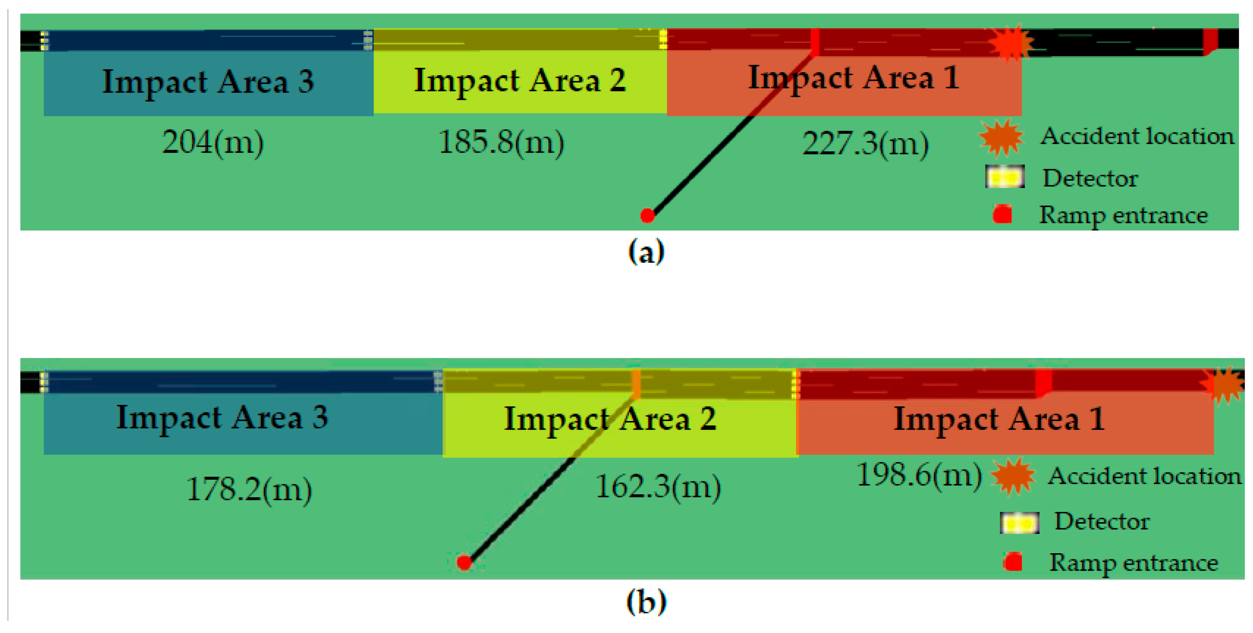
4.3.1. The Risk Propagation of Side Collision Accidents in the Merging Area

Figure 5 shows the changes in the regional risk index for high traffic flow (4770 pcu/h) and low traffic flow (3600 pcu/h) in this scenario. It can be observed that the first impact area, as the area closest to the accident site, always remains at a fluctuating risk level below 1. This indicates that this area is always in a high-risk state. The second impact area is not affected at the beginning of the accident due to its great distance from the accident site. However, with the decline in the regional risk index of the first impact area, the risk in the second impact area increases (see time $t_1$ in Figure 5). Similarly, the third impact area is affected by the risk increase in the second impact area. Its regional risk index starts to decline, which means an increase in risk (see time $t_2$ in Figure 5).

Due to the different input traffic volumes in the experimental scenarios, the beginning time of risk fluctuation in the second and third impact areas are also different. Figure 6 shows the experimental results of the beginning time of risk fluctuation in different traffic volumes. As the traffic volume increases, the fluctuation beginning time of the second impact area becomes earlier. When the input traffic volume is high (4770 pcu/h), the second impact area starts to be affected 200 s after the accident, indicating that the risk spread time from the first impact area to the second impact area is reduced. The third impact area follows a similar pattern. When the traffic volume is high, the risk fluctuation beginning time of the third impact area is affected by the second impact area. Its value is reduced from 600 s to 300 s. Additionally, due to the increase in the input traffic volume, the speed of risk propagation also varies. Figure 7 shows the risk spread speed from the first area to the second and third impact areas in different traffic volumes. The risk spread time from the first impact area to the second impact area is $t_1$. The risk spread time from the second impact area to the third impact area is the difference between $t_1$ and $t_2$. The equation for the speed of risk propagation is as follows:

$$v_1=\frac{s_1}{t_1},v_2=\frac{s_2}{t_2-t_1}$$

(6)

where $v_1$ is the risk spread time from the first impact area to the second impact area; $v_2$ is the risk spread time from the second impact area to the third impact area; $s_1$ is the length of the first impact area; and $s_2$ is the length of the second impact area. The other parameters have been described above.

When the traffic flow is larger than 3900 pcu/h, the risk spread time from the first to the second impact area is greater than that from the second to the third impact area. The propagation speed difference is between 0.2 m/s and 1.3 m/s, which is not significantly related to traffic volume (the Pearson coefficient is −0.11.).

4.3.2. The Risk Propagation of Rear-End Accidents in the Downstream Area

The situation in the first impact area is the same as that of side collision accidents occurring in the merging area. The risk of this area continuously exists after the accident happens. However, the risk levels of the second and third impact areas are different. When traffic flow is low, risk propagation only involves the second impact area. Then, it gradually spreads to the third impact area as the traffic volume increases. In this situation, although the number of lanes is reduced, the lane proportion occupied by accidents is lower in this scenario. Therefore, with the increase in the traffic volume, the second and third impact areas are affected more quickly. The risk exposure moment of the second impact area is relatively small (around 200 s; see Figure 8). However, the risk beginning moment of the third impact area is more obvious from 4000 pcu/h to 4350 pcu/h. It decreases from 900 s to 400 s. Although the traffic flow increases afterwards, the risk beginning moment does not decrease by much (see Figure 8). As shown in Figure 9, in all scenarios, the risk propagation speed from the first to the second impact area is greater than that from the second to the third impact area. The difference is greatest at 4000 pcu/h when the third impact area begins to be affected, and the speed of propagation decreases with the increasing traffic flow.

5. Traffic Accident Risk Prediction Model

In this section, an accident risk prediction model based on the LSTM is built to forecast the accident risk. The input for the model was obtained from the dataset obtained in Section 4, and the training and testing sets were selected based on this dataset. Firstly, the sample data were normalized to ensure the accuracy and stability of the model. Secondly, the LSTM algorithm was applied to train the model and the optimal model parameters were selected. After training, the test set was fed into the prediction model, and the test results were denormalized to obtain the actual predicted values. Finally, the error analysis was presented to verify its effectiveness and accuracy. The above process is shown in Figure 10.

5.1. Model

5.1.1. LSTM

Risk propagation is a dynamic process, where future risks may be influenced by past risks and have a cumulative effect over time. Traditional statistical models cannot accurately model this dynamic and complex nature, but LSTM (long short-term memory) model, as a deep learning model suitable for modeling sequence data, can effectively solve this problem. An LSTM model can store previous information and predict future risk trends, making it widely applicable in risk forecasting [34]. It is capable of modeling time series data and handling long-term dependencies in sequence data. This makes it particularly suitable for risk prediction, as the time accumulation effect of risk propagation requires a model that can identify and handle long-term dependencies in sequence data. Therefore, the memory and long-term dependency processing capabilities of LSTM models make them a highly suitable tool for risk prediction. An LSTM model introduces “gates” to control the flow of information, which allows the network to selectively remember or forget previous information.

The core of LSTM is the cell, which is controlled by three gates: the input gate, the forget gate, and the output gate. The input gate controls the input of new information, the forget gate controls the forgetting of old information, and the output gate controls the output of the cell state. The specific steps are as follows:

(1)

The input gate controls the input of new information by multiplying the input vector with the weight matrix through sigmoid function to produce a numerical vector between 0 and 1.

(2)

The forget gate controls the forgetting of old information by multiplying the input vector with the weight matrix through sigmoid function to produce a numerical vector between 0 and 1. This vector will be element-wise multiplied with the cell state vector to determine which old information should be forgotten.

(3)

The cell state is updated by element-wise multiplying the vector generated by the forget gate with the cell state from the previous time step to obtain the old information that needs to be retained and multiplying the vector generated by the input gate with the new information processed by a function element-wise to obtain the new information that needs to be added. These two vectors are added together to obtain the updated cell state.

(4)

The output gate controls the output of the cell state by multiplying the input vector with the weight matrix through sigmoid function to produce a numerical vector between 0 and 1. This vector is then element-wise multiplied with the cell state vector processed by a function to obtain the final output vector.

Assuming the current time series is $t$ and the data input is $x$, the predicted output is $h$, and $c$ is the memory cell. The network structure can be constructed as Figure 11.

In Figure 11, $\sigma$ represents the sigmoid activation function; $[h_{t-1},x_t]$ is the composite matrix of the previous prediction result $h_{t-1}$ and the input parameter $x_t$ in this round, which is the input parameter at time $t$; $W_t$ is the forget gate weight matrix; $W_c$ is the output weight matrix; and $W_o$ is the current state control matrix. The numerical expressions of the forget, input, control, and output gates can be represented by Equations (7)–(11):

$$f_t=\sigma (W_f[h_{t-1},x_t]+b_f)$$

(7)

$$i_t=\sigma (W_t[h_{t-1},x_t]+b_i)$$

(8)

$$c_t=f_t{c}_{t-1}+\tan (W_c[h_{t-1},x_t]+b_c)$$

(9)

$$o_t=\sigma (W_o[h_{t-1},x_t]+b_o)$$

(10)

$$h_t=o_t\tanh (c_t)$$

(11)

where $b_f$, $b_i$, $b_c$, and $b_o$ are bias vectors for the forget, input, control, and output gates, respectively. All other parameters have been described above.

5.1.2. RNN

In addition to the LSTM model, a recurrent neural network (RNN) model was also applied for comparison in this study. A RNN is a type of neural network that can handle time-dependent relationships in sequence data. Unlike traditional feedforward neural networks, RNN has a feedback loop that allows information to be passed from one step of the sequence to the next. This allows the model to capture information about the sequence’s history to make predictions.

RNNs are prone to the vanishing or exploding gradient problem when dealing with long-term dependencies in sequence data, which can limit their performance in certain scenarios [35]. In contrast, LSTM is designed to mitigate this issue by incorporating memory units and gating mechanisms, which allows the model to selectively remember or forget information as needed.

5.2. Dataset

The dataset used was derived from the simulation data in Section 4. Since the dataset did not include information about the accidents themselves, current traffic flow, the accident lane, the accident location in the merging area, and the type of accident as categorical variables were added to reflect the impact of the accident (as shown in

Table 3. Input variable and explanation.

Variable Name	Explanation
Traffic_flow_all	Initial traffic volume in the simulation scenario
Speed_1	Average speed of vehicles passing through the first impact area
Speed_2	Average speed of vehicles passing through the second impact area
Speed_3	Average speed of vehicles passing through the third impact area
Traffic_flow_1	Number of vehicles passing through the first impact area
Traffic_flow_2	Number of vehicles passing through the second impact area
Traffic_flow_3	Number of vehicles passing through the third impact area
RL1	Regional risk index for the first impact areas
RL2	Regional risk index for the second impact areas
RL3	Regional risk index for the third impact areas
Location	Categorical variable, 1 if the accident is in the merging areas, 0 otherwise
Lane1	Categorical variable, 1 if the accident occurred in lane 1, 0 otherwise
Lane2	Categorical variable, 1 if the accident occurred in lane 2, 0 otherwise
Lane3	Categorical variable, 1 if the accident occurred in lane 3, 0 otherwise
Lane4	Categorical variable, 1 if the accident occurred in lane 4, 0 otherwise

). These additional variables could reflect the situation of traffic accidents more specifically and help to improve the prediction accuracy of the model.

5.3. Model Parameters

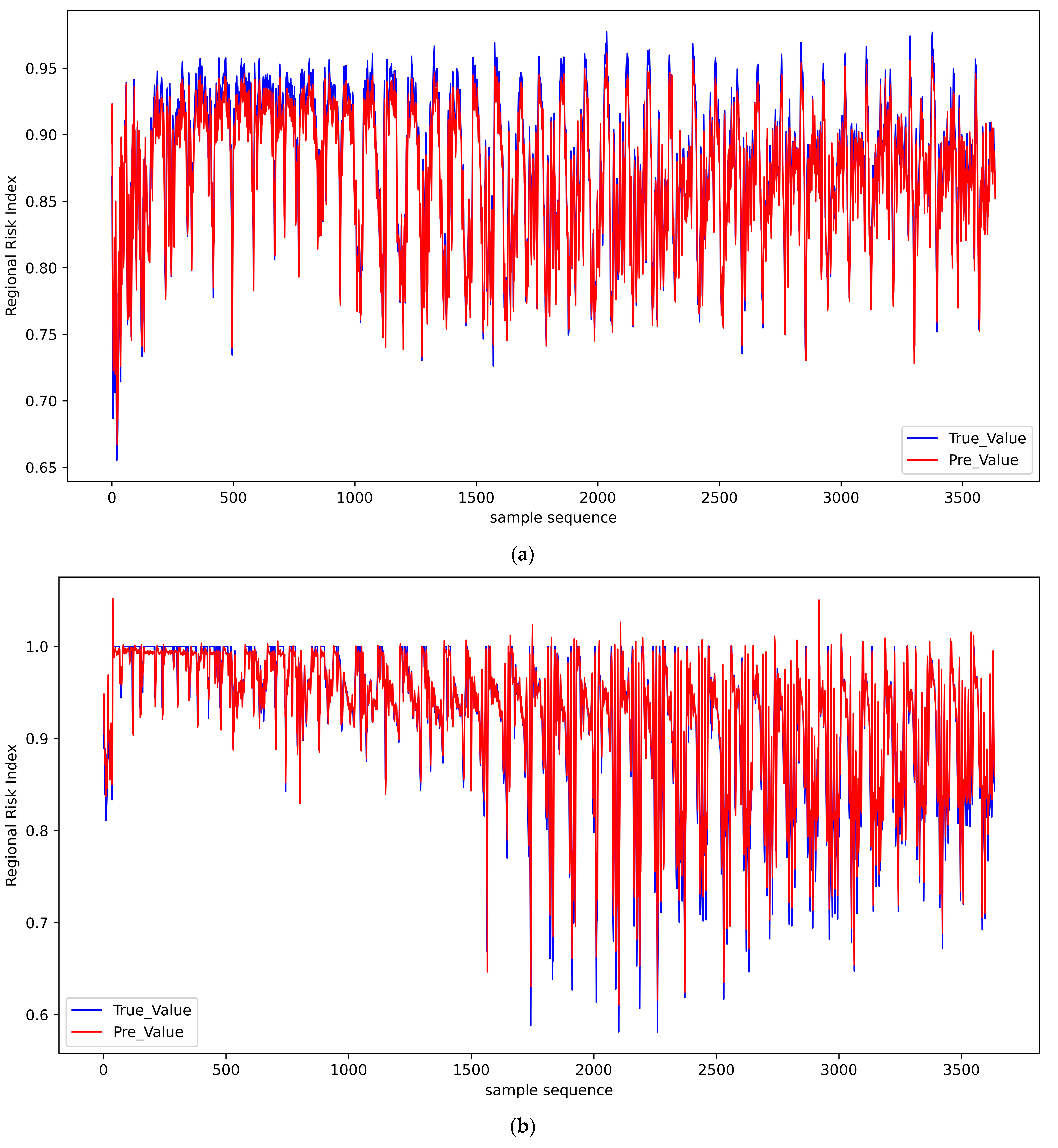
The dataset in Section 4 is split into a training set (80%) and a validation set (20%). The mean squared error (MSE) function was used as the loss function to measure the error between the predicted and true values during LSTM model training. In the deep learning algorithm, calculating the difference between the learning results and the sample labels is an important step. The smaller the difference, the better the learning effect. This difference is the loss value. In this study, the MSE function was used as the loss function, which was suitable for solving regression problems and to evaluate the predictive performance of the model on the training and validation sets. The grid search method was used to determine the super parameter values of the LSTM model. The super parameter values of the model are shown in

Table 4. Parameter values of the model.

Number of Neurons.	Optimizer	Activation Function	Learning Rate	Batch Size	Epoch	Dropout
50	ADAM	Sigmoid	0.01	120	50	0.2

.

This study uses root mean square error (RMSE), mean squared error (MSE), and mean absolute error (MAE) [36] to evaluate the accuracy of the model (see Equations (12)–(14)).

$$RMSE=\sqrt{\frac{1}{n}\sum _{i=1}^n{\left({\widehat{y}}_i-y_i\right)}^2}$$

(12)

$$MSE=\frac{1}{n}\sum _{i=1}^n{\left({\widehat{y}}_i-y_i\right)}^2$$

(13)

$$MAE=\frac{1}{n}{\displaystyle \sum _{i=1}^n|{\widehat{y}}_i-y_i|}$$

(14)

where $y_i$ is the true value and ${\widehat{y}}_i$ is the predicted value.

MSE, RMSE, and MAE are used in regression analysis to measure the difference between predicted and actual values. All three values fall into the interval [0, +∞), indicating that the difference cannot be negative, and a lower value indicates better model performance.

5.4. Model Results

The predicted values and actual values of the regional risk index for the first, second, and third impact areas are shown in Figure 12. It can be observed that in each experiment, there is a certain amount of fluctuation in the prediction results, which is the beginning and end of each experiment. In order to validate the performance of the proposed model, this study selected the RNN model and the LSTM model for training and testing the data samples and compared the risk prediction accuracy in the merging area.

Table 5. Prediction performance of the LSTM and RNN models for different impact areas.

Impact Area	Model	RMSE	MSE	MAE
1	LSTM	0.0153	0.0002	0.0122
	RNN	0.0212	0.0004	0.0189
2	LSTM	0.0219	0.0005	0.0136
	RNN	0.0337	0.0011	0.0215
3	LSTM	0.0158	0.0002	0.0146
	RNN	0.0241	0.0005	0.0198

presents a comparison of the prediction results between the RNN model and the LSTM model. It shows that the LSTM model outperforms the RNN model in all three evaluation indicators, with an improvement of over 20% in each indicator. It also suggests that the LSTM model is more suitable for traffic risk prediction tasks due to its ability to capture long-term dependencies in the data. Therefore, the LSTM model results in more accurate and reliable predictions.

Specifically, Table 5 presents the performance of two different models (LSTM and RNN) across three different impact areas. It can be observed that the LSTM model consistently outperforms the RNN model in all three impact areas, with significantly lower RMSE, MSE, and MAE values. Moreover, the performance of the two models varies across the different impact areas. For instance, in impact area 1, the RMSE, MSE, and MAE of LSTM are 27.8%, 50.0%, and 35.4% lower than those of the RNN model, respectively. Similarly, in impact area 2, the LSTM model performs better than the RNN model, with 35.0%, 54.5%, and 36.7%, respectively. In impact area 3, the LSTM model performs better with 34.4%, 60.0%, and 26.36%, respectively. In summary, these findings indicate that the LSTM model performs much better than the RNN model in predicting the regional risk index in all impact areas.

6. Conclusions

This study proposes the concept of risk propagation in highway merging areas. A Gaussian-plume-model-based accident impact range model is proposed, which clarifies the impact range of accidents and divides the impact area into three levels. In order to study the risk propagation of each level, a series of simulation experiments were conducted in the highway merging situation. The risk propagation speed was studied through the regional risk index. Therefore, the following conclusions can be drawn.

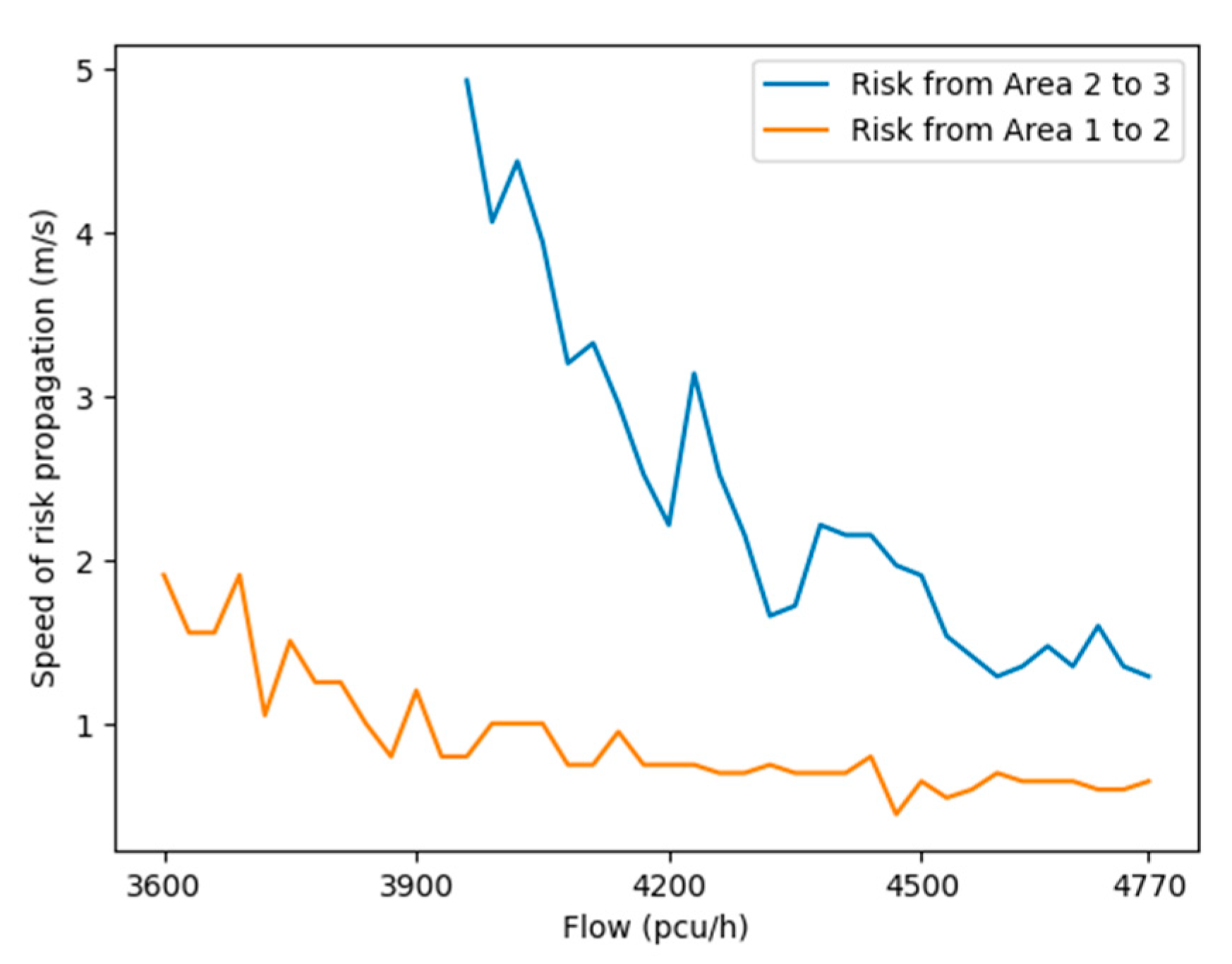
• The simulation results show that the risk of the first impact area remained high throughout the experiment. As the regional risk index in the first impact area decreased, the risk in the second and third impact areas increased. This means that the accident risk spreads from the first impact area to the following areas, which verifies the risk propagation phenomenon of accidents. The risk spreading time from one area to another was affected by traffic flow. Specifically, as traffic flow increases, the risk spread time from the first to second impact areas decreased. This indicates that accidents could spread more quickly in high traffic flow scenarios. The risk spread time from the second to third impact areas also decreased with increasing traffic flow. However, the speed of risk propagation between the second and third impact areas was generally faster than that between the first and second impact areas.
• The risk propagation speed of different impact levels is related to the accident location. Specifically, when the accident occurs downstream of the merging area, it takes longer for the risk to propagate from the first-level impact area to the second-level impact area compared to the spread time from the second-level impact area to the third-level impact area. However, when an accident occurs in the merging area, the situation is quite the opposite. This is because when the accident occurs downstream, part of the second-level impact area is in the merging area where there are fewer lanes and a higher likelihood of accidents. In contrast, the downstream area of the merging area has more lanes, larger vehicle gaps and lower vehicle speed. This makes it safer to drive. As a result, the risk takes more time to spread from the first-level to the second-level impact area.
• Furthermore, this study proposed a high-speed highway merging risk prediction model based on LSTM. The model performed well in predicting collision risk. It can be used by researchers and practitioners to predict and monitor highway merging risk accurately. Therefore, different control measures can be taken for different impact areas to achieve precise control and reduce the risk of traffic accidents.

However, this study has the following limitations, which need to be improved in future research. The traffic data used in this study were not collected from real highway segments, so the real driving behavior may differ from the simulation results. Therefore, the experiments in this study cannot fully reproduce the real merging situations. In addition, although rear-end and side collisions are the most common collision types in highway merging areas, other collision types should be considered in future research to improve the risk warning mechanism.

References

1. Michalopoulos, P.M.; Pisharody, V.B. Derivation of delays based on improved macroscopic traffic models. Transp. Res. Part B 1981, 15, 299–317. [Google Scholar] [CrossRef]
2. Sheu, J.; Chou, Y.; Chen, A. Stochastic modeling and real-time prediction of incident effects on surface street traffic congestion. Appl. Math. Model. 2004, 28, 445–468. [Google Scholar] [CrossRef]
3. Deo, C.; Boniphace, K.; Gary, O. Impact of Abandoned and Disabled Vehicles on Freeway Incident Duration. J. Transp. Eng. 2014, 140, 40130131. [Google Scholar]
4. Lawson, T.W.; Lovell, D.J.; Daganzo, C.F. Using Input-Output Diagram to Determine Spatial and Temporal Extents of a Queue Upstream of a Bottleneck. Transp. Res. Rec. 1996, 1572, 140–147. [Google Scholar] [CrossRef] [Green Version]
5. Smid, R.M. The Variability of Traffic in Congestion Forecasting. Master’s Thesis, Delft University of Technology, The Hague, The Netherlands, 2012. [Google Scholar]
6. Khattak, A.; Wang, X.; Zhang, H. Incident management integration tool: Dynamically predicting incident durations, secondary incident occurrence and incident delays. Intell. Transp. Syst. IET 2012, 6, 204–214. [Google Scholar] [CrossRef]
7. Chung, Y.; Recker, W.W. A Methodological Approach for Estimating Temporal and Spatial Extent of Delays Caused by Freeway Accidents. IEEE Trans. Intell. Transp. Syst. 2012, 13, 1454–1461. [Google Scholar] [CrossRef]
8. Zhang, J.; Zhang, L.; Dong, X. Forecasting Method of Traffic Accident Impact Sphere of Expressway Network. J. East China Jiaotong Univ. 2017, 34, 85–91. [Google Scholar]
9. Hu, X.; Wang, W. Determination impact of traffic accident. J. Southeast Univ. 2007, 5, 198–201. [Google Scholar]
10. Li, X. Determination Impact of Traffic Accident. Master’s Thesis, Chongqing Jiaotong University, Chongqing, China, 2015. [Google Scholar]
11. Yu, B.; Lu, J. Method to Determine the Influence Area of Street Accidents. Urban Transp. 2008, 3, 82–86. [Google Scholar]
12. Li, M.; Zhu, Y. Coverage Analysis and Simulation Study for Traffic Flow afterTraffic Accidents on Expressways. J. Highw. Transp. Res. Dev. 2012, 6, 109–111. [Google Scholar]
13. Ma, A. Study on the Freeway Traffic Accident Duration and Influence Range. Master’s Thesis, Chang’an University, Chang’an, China, 2013. [Google Scholar]
14. Lin, H. Study on Key Problems of Freeway Traffic Emergency Disposal. Master’s Thesis, Chang’an University, Chang’an, China, 2018. [Google Scholar]
15. Jin, S.; Wang, W. Traffic accident affected zone division and traffic guidance under regional highway network. J. Chang’an Univ. 2017, 37, 89–98. [Google Scholar]
16. Hossain, M.; Muromachi, Y. A Bayesian network based framework for real-time crash prediction on the basic freeway segments of urban expressways. Accid. Anal. Prev. 2012, 45, 373–381. [Google Scholar] [CrossRef]
17. Zhai, B.; Lu, J.; Wang, Y. Real-time prediction of crash risk on freeways under fog conditions. Int. J. Transp. Sci. Technol. 2020, 9, 287–298. [Google Scholar] [CrossRef]
18. Sun, J.; Sun, J. A dynamic Bayesian network model for real-time crash prediction using traffic speed conditions data. Transp. Res. Part C Emerg. Technol. 2015, 54, 176–186. [Google Scholar] [CrossRef]
19. Chen, X.; Wang, Z.; Hua, Q.; Shang, W. AI-Empowered Speed Extraction via Port-Like Videos for Vehicular Trajectory Analysis. IEEE Trans. Intell. Transp. Syst. 2023, 24, 4541–4552. [Google Scholar] [CrossRef]
20. Yang, K.; Zhao, W.; Antoniou, C. Utilizing Import Vector Machines to Identify Dangerous Pro-active Traffic Conditions. In Proceedings of the International Conference on Intelligent Transportation Systems (ITSC), Rhodes, Greece, 1–6 September 2020. [Google Scholar]
21. Zhang, J.; Hu, Z.; Zhu, X. Real-time traffic accident prediction based on AdaBoost classifier. J. Comput. Appl. 2017, 37, 284–288. [Google Scholar] [CrossRef]
22. Qu, X.; Wang, W.; Wang, W. Real-time rear-end crash potential prediction on freeways. J. Cent. South Univ. 2017, 24, 2664–2673. [Google Scholar] [CrossRef]
23. Fu, C.; Wang, J. A real-time accident risk model on freeways based on monitoring data. J. Transp. Inf. Saf. 2017, 35, 11–17. [Google Scholar]
24. Zhou, Z.; Wang, Y.; Xie, X.; Chen, L.; Liu, H. RiskOracle: A Minute-level Citywide Traffic Accident Forecasting Framework. In Proceedings of the AAAI Conference on Artificial Intelligence, New York, NY, USA, 7–12 February 2020. [Google Scholar]
25. Yuan, Z.; Zhou, X.; Yang, T. Hetero-ConvLSTM: Hetero-ConvLSTM: A Deep Learning Approach to Traffic Accident Prediction on Heterogeneous Spatio-Temporal Data. In Proceedings of the 24th ACM SIGKDD International Conference on Knowledge Discovery & Data Mining, London, UK, 19–23 August 2018. [Google Scholar]
26. Yu, L.; Du, B.; Hu, X.; Sun, L.; Han, L.; Lv, W. Deep spatio-temporal graph convolutional network for traffic accident prediction. Neurocomputing 2021, 423, 135–147. [Google Scholar] [CrossRef]
27. Ren, H.; Song, Y.; Wang, J.; Wang, J.; Lei, J. A Deep Learning Approach to the Citywide Traffic Accident Risk Prediction. In Proceedings of the 21st International Conference on Intelligent Transportation Systems (ITSC), Maui, HI, USA, 4–7 November 2018. [Google Scholar]
28. Chen, Q.; Song, H.; Yamada, H.; Shibasaki, R. Learning Deep Representation from Big and Heterogeneous Data for Traffic Accident Inference. In Proceedings of the 30th AAAI Conference on Artificial Intelligence, Phoenix, AZ, USA, 12–17 February 2016. [Google Scholar]
29. Zhu, S.; Jiang, R. Review of Research on Traffic Conflict Techniques. J. Highw. Transp. 2020, 33, 15–33. [Google Scholar]
30. Pasquill, F.; Smith, F.B. The Determination of the Dispersion of Windborne Material. Meteorol. Mag. 1961, 90, 33–49. [Google Scholar]
31. Yang, L.; Luo, X.; Zuo, Z.; Zhou, S.; Huang, T.; Luo, S. A novel approach for fine-grained traffic risk characterization and evaluation of urban road intersections. Accid. Anal. Prev. 2023, 181, 106934. [Google Scholar] [CrossRef] [PubMed]
32. Wang, J.; Wang, S.; Long, X.; Li, D.; Ma, C.; Li, P. Ellipse-Like Radiation Range Grading Method of Traffic Accident Influence on Mountain Highways. Sustainability 2022, 14, 13727. [Google Scholar] [CrossRef]
33. Yang, F. Accident Prediction and Safety Hazards Digging of Ordinary Arterial Highway in Mountain Area Based on Accident Scenario Classification. Doctor Thesis, Chang’an University, Chang’an, China, 2021. [Google Scholar]
34. Greff, K.; Srivastava, R.K.; Koutník, J.; Steunebrink, B.R.; Schmidhuber, J. LSTM: A search space odyssey. IEEE Trans. Neural Netw. Learn. Syst. 2016, 28, 2222–2232. [Google Scholar] [CrossRef] [Green Version]
35. Sutskever, I.; Martens, J.; Dahl, G.; Hinton, G. On the difficulty of training recurrent neural networks. In Proceedings of the 30th International Conference on Machine Learning (ICML-13), Atlanta, GA, USA, 16–21 June 2013. [Google Scholar]
36. Chen, X.; Wu, X.; Prasad, D.; Wu, B. Pixel-Wise Ship Identification From Maritime Images via a Semantic Segmentation Model. IEEE Sens. J. 2022, 22, 18180–18191. [Google Scholar] [CrossRef]
Figure 1. The accident impact illustration of the highway merging area.
Applsci 13 08014 g001
Figure 2. Schematic diagram of accident risk propagation.
Applsci 13 08014 g002
Figure 3. Simulation scenario: (a) merging area and (b) downstream.
Applsci 13 08014 g003
Figure 5. The risk values for first-, second-, and third-level impact areas. (a) Low traffic flow. (b) High traffic flow.
Applsci 13 08014 g005
Figure 6. The risk exposure moment of the second- and third-level impact areas (side collision).
Applsci 13 08014 g006
Figure 7. The speed of risk propagation in the second- and third-level impact areas (side collision).
Applsci 13 08014 g007
Figure 8. The risk exposure moment of the second- and third-level impact areas (rear-end collision).
Applsci 13 08014 g008
Figure 9. The speed of risk propagation in the second- and third-level impact areas (rear-end collision).
Applsci 13 08014 g009
Figure 10. Flowchart of the traffic accident risk prediction model.
Applsci 13 08014 g010
Figure 11. The structure of the LSTM model.
Applsci 13 08014 g011
Figure 12. The predicted values and actual values of the regional risk index as forecasted by the LSTM model. (a) The first impact area. (b) The second impact area. (c) The third impact area.
Applsci 13 08014 g012aApplsci 13 08014 g012b