DANet: Temporal Action Localization with Double Attention

Abstract

Temporal action localization (TAL) aims to predict action instance categories in videos and identify their start and end times. However, existing Transformer-based backbones focus only on global or local features, resulting in the loss of information. In addition, both global and local self-attention mechanisms tend to average embeddings, thereby reducing the preservation of critical features. To solve these two problems better, we propose two kinds of attention mechanisms, namely multi-headed local self-attention (MLSA) and max-average pooling attention (MA) to extract simultaneously local and global features. In MA, max-pooling is used to select the most critical information from local clip embeddings instead of averaging embeddings, and average-pooling is used to aggregate global features. We use MLSA for modeling local temporal context. In addition, to enhance collaboration between MA and MLSA, we propose the double attention block (DABlock), comprising MA and MLSA. Finally, we propose the final network double attention network (DANet), composed of DABlocks and other advanced blocks. To evaluate DANet’s performance, we conduct extensive experiments for the TAL task. Experimental results demonstrate that DANet outperforms the other state-of-the-art models on all datasets. Finally, ablation studies demonstrate the effectiveness of the proposed MLSA and MA. Compared with structures using backbone with convolution and global Transformer, DABlock consisting of MLSA and MA has a superior performance, achieving an 8% and 0.5% improvement on overall average mAP, respectively.

1. Introduction

With the rapid development of media, the amount of video data is increasing exponentially in real life. Therefore, the research topic of video understanding has received much attention [1,2,3], especially temporal action localization (TAL), which is a fundamental task in the field of video understanding. TAL aims to predict the semantic labels of actions and their corresponding start and end times, which provides convenience for the development of various applications such as video recommendation, security monitoring, and sports analysis.

To solve TAL tasks better, many two-stage and one-stage methods have been proposed [4,5,6,7,8,9,10,11,12,13,14,15,16]. The two-stage TAL methods [7,17] follow a proposal-then-classification paradigm, where generating high-quality action proposals is fundamental for their high-level performance. Different from two-stage methods, one-stage ones [8,18] aim to localize actions in a single shot without requiring any action proposals. Many one-stage methods are anchor-based and adjust predefined anchors to perform action localization [8]. However, because the anchors are fixed, the anchor-based approaches lack flexibility in adapting to various action classes. Recently, to capture semantic information better, many anchor-free methods [5,10] have been proposed to localize actions. Specifically, they classify each time step in videos and generate behavior boundaries. In addition, recently many anchor-free methods have adopted Transformer [19] as their backbone, because Transformer with self-attention mechanisms can better capture and model information for video sequences.

However, methods leveraging global self-attention (e.g., [9]) may ignore local variances, which may potentially result in poor performance. To solve this problem, local self-attention mechanisms have been employed in some methods (e.g., [10]), which may result in the loss of some global information. Additionally, both global and local self-attention methods have been found to conflate the embeddings of segments within a given attention range, and thereby may reduce the discriminative quality of these features [20]. To pursue high performance, preserving the most salient traits of local clip embeddings is crucial [21].

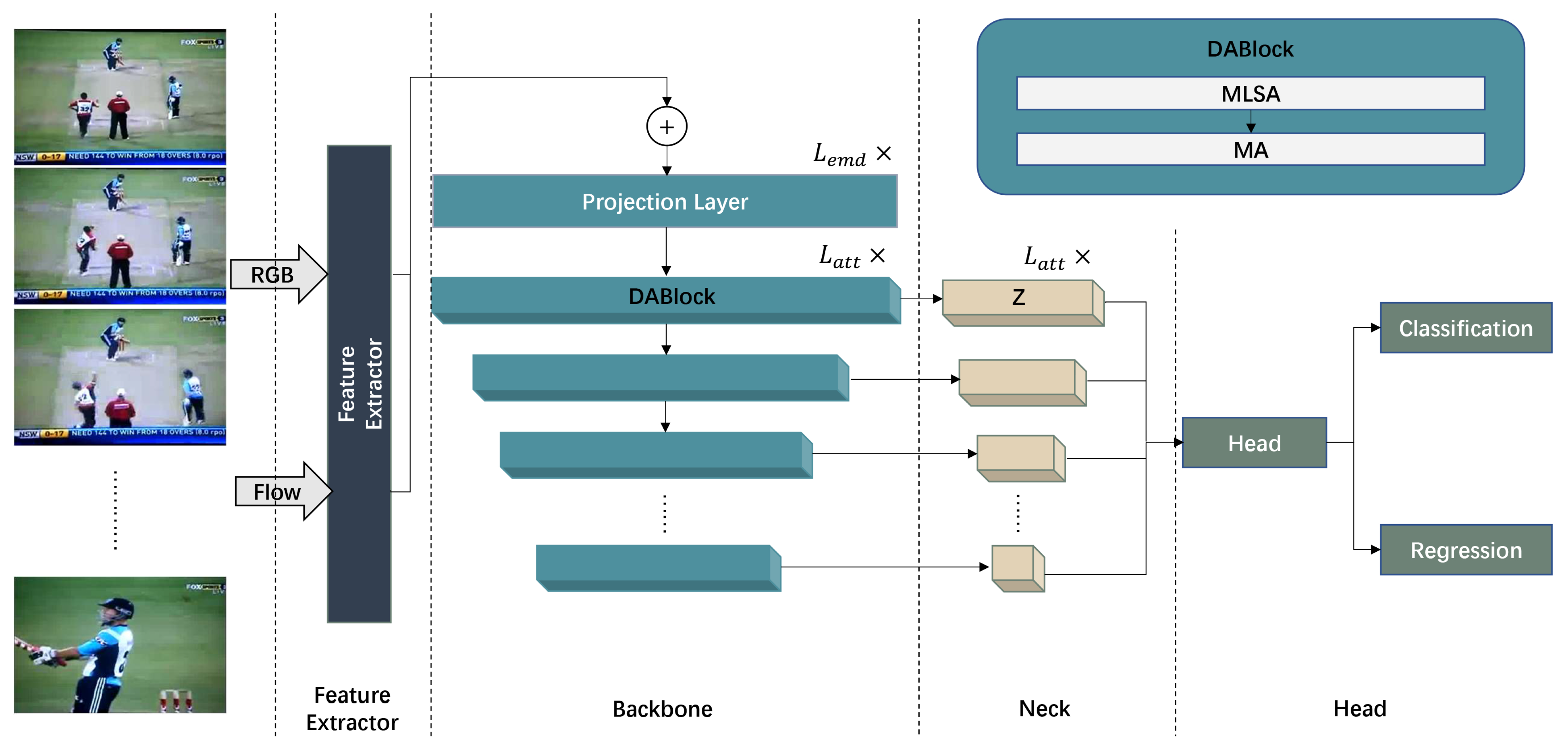
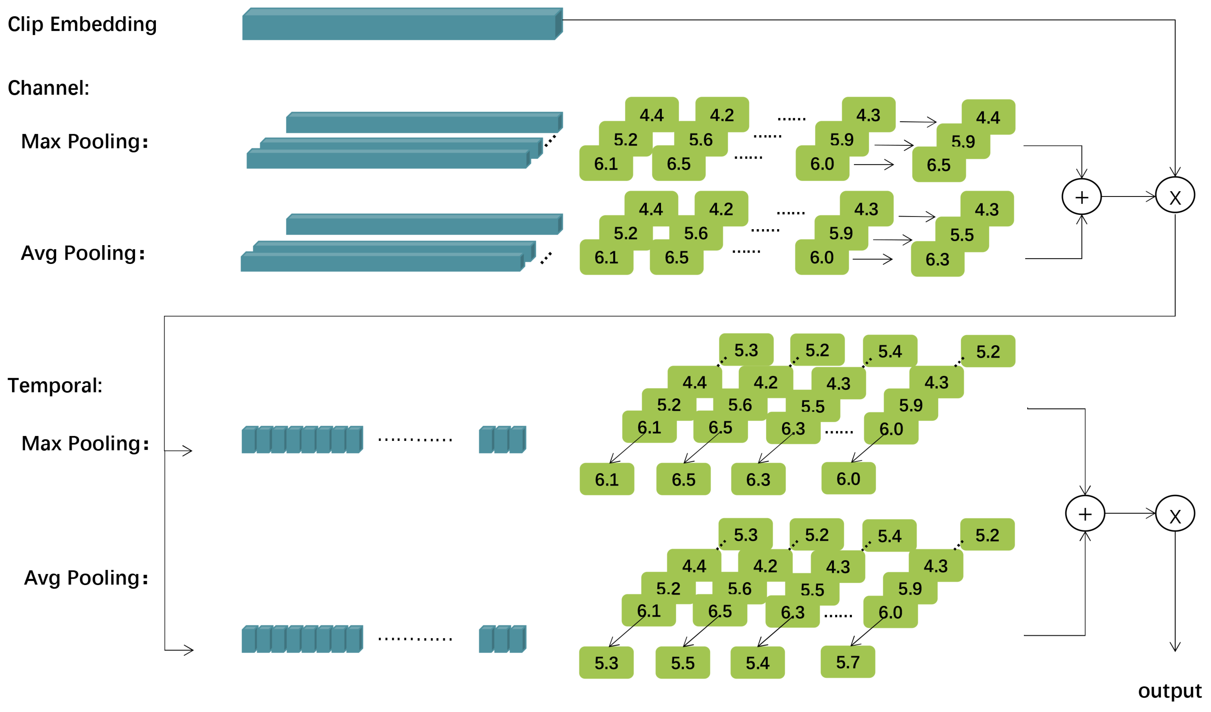
Therefore, to facilitate more comprehensive modeling of temporal information, we propose a model named the double attention network (DANet), comprising more advanced blocks, e.g., double attention block (DABlock), featurized image pyramid (FIP), and classification and regression head (CRHead). Specifically, to model both global and local information simultaneously and maintain the most salient traits of local clip embeddings, we design two attention mechanisms for DABlock, namely multi-headed local self-attention (MLSA) and max-average pooling attention (MA). Among these, MLSA only models local temporal context, while MA extracts information from local clip embeddings and aggregates global information. Specifically, MA retains the most critical features from local embeddings by using max-pooling and also aggregates global features by average-pooling and generates corresponding attention weights (see Section 3.2 for more details). Adopting these kind of attention mechanisms can help preserve all the discriminative information of local clip embeddings. In addition, we adopt the FIP as the neck of model to focus better local changes and use CRHead to predict the semantic labels of actions (see Section 3.3 and Section 3.4 for more details).

To assess the performance of DANet, we conduct extensive experiments on two TAL task datasets, namely THUMOS14 [22] and ActivityNet1.3 [23] datasets. On the THUMOS14 dataset, DANet achieves a mean average precision (mAP) of 66.56%, a mAP of 78.2% at the time Intersection over Union (tIoU) = 0.4, and a mAP of 58.7% at tIoU = 0.6. Compared with the state-of-the-art method ActionFormer [10], for average mAP and mAP at tIoU of 0.4 and 0.6, respectively, our method outperforms ActionFormer by over one percentage point. In addition, DANet also outperforms all two-stage methods such as AFSD [5], PBRNet [24], and GTAN [8], as well as the other one-stage methods such as RTD-Net [25], ContextLoc [26], BMN-CSA [27], and MUSES [6]. In addition, through conducting comprehensive ablation studies, we not only demonstrate the effectiveness of MLSA and MA, but also investigate the impact of some hyper-parameters on the experimental results, such as the number of projection layers, path aggregation, and the adopted normalization method (see Section 4.3).

The key contributions of this work are as follows:

• To enable comprehensive contextual modeling of temporal information, we propose a model named DANet comprising MLSA and MA. MLSA models temporal context by local self-attention. MA aggregates global feature information.
• To preserve the salient characteristics of local clip embeddings, MA returns discriminative features by using max-pooling in both channel and temporal dimensions as well as generates attention weights.
• Compared with other methods, DANet achieves the best performance on THUMOS14 and ActivityNet1.3 datasets. In addition, ablation studies demonstrate the effectiveness of MLSA and MA as well as the adopted hyper-parameters.

2. Related Work

In this section, we first introduce a brief overview of existing TAL methods. Then we give a concise introduction to the recently popular Vision Transformer [19] approaches applied in TAL.

2.1. Temporal Action Localization

Existing TAL methods can be broadly divided into two categories, i.e., two-stage methods [6,7,17] and one-stage methods [8,9,10,18]. The two-stage approaches [6,7,17] solve the TAL task by first proposing location proposals of action instances and subsequently using the location proposals to predict the semantic labels of actions and their corresponding start and end times. For example, BSN [4] first localizes the boundaries with a higher possibility, and then merges those boundaries to derive location proposals. Subsequently, BSN employs the temporal proposals to determine whether an action instance is present or not and computes the confidence of the temporal proposals. However, the efficiency of BSN is not high enough because feature extraction and confidence assessment are performed for each temporal proposal, leading to a potentially time-consuming process. To solve the corresponding limits, BMN [7] is proposed, which can simultaneously generate the probability of one-dimensional boundaries and the confidence maps. However, two-stage methods separate proposal and classification tasks, which may be inefficient and time-consuming [28].

Compared with two-stage approaches, one-stage ones [8,9,10,18] possess a more notable and simple pipeline, because one-stage methods eliminate the proposal generation process utilized in the two-stage methods. Furthermore, one-stage methods can be broadly divided into two categories, namely, anchor-based [8] and anchor-free methods [5]. For instance, SSAD [18] is a monolithic anchor-based network that directly predicts the timing boundaries and the confidence of actions. Conversely, the anchor-free approach is frame-level, wherein each time node is generally predicted, and eventually merged at the frame-level to generate the final prediction. For example, ActionFormer [10], an anchor-free approach, combines multi-scale feature representation with self-attention, uses a weighted decoder to classify each time step, and estimates the corresponding action boundaries. However, ActionFormer limits self-attention in a local window, which may be unable to integrate global information of a video effectively and capture all relevant time intervals (see Section 4.2).

Our model is a one-stage, anchor-free approach, which classifies each time step and generates behavior boundaries, followed by the merging of frame-level results to produce the final output. Specifically, we model temporal context at both local and global levels simultaneously.

2.2. Vision Transformer in Video Understanding

Transformer [19] has shown superior performance in the field of natural language processing (NLP), which is at the center stage of data-driven artificial intelligence. As the key component in Transformer, the self-attention mechanism enables the establishment of long-term context reliance on the input sequence. Subsequently, many researchers in NLP [29,30,31,32] incorporate Transformer into their methods to yield groundbreaking performance. Furthermore, to achieve better performance, many methods [33,34] incorporate Transformer into the field of computer vision (CV) (e.g., Vision Transformer (ViT) [33]). Specifically, ViT transforms the input image into a sequence of tokens for the input model by dividing the image into small pieces, adding extra learnable class embeddings, and feeding them into stacked Transformer blocks. In addition, many Transformer-based models [35,36] have been proposed to solve video understanding tasks.

However, most Transformer-based methods adopt the global self-attention mechanism, which may ignore local variations and thus affect the inference of the boundary timestamps for action instances. Therefore, some Transformer-based methods adopt the local self-attention mechanism, rather than the global self-attention mechanism. However, adopting the local self-attention mechanism cannot accurately capture all relevant time intervals and action instances. Obviously, capturing both global and local information simultaneously is key. To capture the most critical local features and model global contextual of temporal information, we propose two kinds of mechanisms (see Section 3.2 for more details).

3. Double Attention Network

We propose DANet to strive for better performance by extracting global and local information simultaneously and maintaining discriminative features. In this section, we first present the process of feature extraction. Then, we propose a novel block, named DABlock, consisting of dual-attention mechanisms named MLSA and MA to model temporal context. Subsequently, we introduce the design of neck and the structure of head. Finally, we present the loss function we used to supervise the training of DANet better. In Figure 1, we illustrate overview of the proposed DANet, which comprises four key components, namely feature extraction, backbone, neck, and head modules.

3.1. Feature Extraction

Let an untrimmed dataset be denoted as $\mathcal{T}$. For each video in the dataset $\mathcal{T}$, we extract a number of J RGB frames and a number of J optical flows, and then perform separate feedforward passes through a pre-trained 3D CNN network (e.g., I3D [37]) fine-tuned on kinetics. Subsequently, we merge the resulting RGB frames and optical flows into input feature vectors, denoted as $X=\{x_1,x_2,\dots ,x_T\}$, where $X\in {\mathbb{R}}^{T\times C_{\mathrm{org}}}$, $C_{\mathrm{org}}$ denotes the dimensions of the input feature vectors, and T depends on the video length.

3.2. Double Attention Block

The backbone module consists of a number of $L_{\mathrm{emd}}$ projection layers denoted as E and a number of $L_{\mathrm{att}}$ DABlock layers. Specifically, each projection layer contains a 1D convolutional neural network followed by layer normalization and RELU. Let the output of all projection layers be denoted by P, which is given by:

$$P=E\left(X\right),$$

(1)

where $P\in {\mathbb{R}}^{T\times C_{\mathrm{emd}}}$ and $C_{\mathrm{emd}}$ denotes the dimension of all projection layers. T varies depending on the video length. Subsequently, the output of all projection layers, P, is used as the input of the 0th DABlock $D^0$. In addition, let $D^i$ denote the input of the ith DABlock, where $i\in \{0,1,\dots ,L_{\mathrm{a}tt}-1\}$.

As shown in Figure 1, the DABlock comprises two attention modules that capture the local and global temporal relationships in an untrimmed video, named MLSA and MA. In MLSA, to focus on the local temporal context and enhance local awareness, we employ multi-headed self-attention to model temporal relationships, which is computed as follows:

$$S=\mathit{softmax}(Q{K}^T/\sqrt{D_q})V,$$

(2)

where $Q=D^i{W}_Q,K=D^i{W}_K,V=D^i{W}_V$, and are referred to as query, key, and value, respectively. $W_Q\in {\mathbb{R}}^{C_{\mathrm{emd}}\times C_q},W_K\in {\mathbb{R}}^{C_{\mathrm{emd}}\times C_k},W_V\in {\mathbb{R}}^{C_{\mathrm{emd}}\times C_v}$ denote the weight of query, key, and value, respectively. Multi-headed self-attention performs self-attention operations on $N_{\mathrm{head}}$ heads in parallel, and thus has $C_{\mathrm{emd}}/N_{\mathrm{head}}$ channels at each head. After calculation, let $h_m^i$ denote the output of the mth head. Therefore, the output of the ith MLSA is as follows:

$$M^i=\mathit{Concat}(h_1^i,h_2^i,\dots ,h_{N_{\mathrm{head}}}^i).$$

(3)

To preserve the most critical local features and aggregate global feature information, we propose MA, whose structure is illustrated in Figure 2. We apply MA to maintain the discriminative features from local embeddings through the use of max-pooling, while aggregating global feature information via average-pooling. In addition, we apply polling operations on both the channel and temporal dimensions and generate corresponding attention weights.

Specifically, for the channel-wise attention weights, we utilize max-pooling to preserve the most salient traits of local clip embeddings. We employ average-pooling to aggregate information for each channel. Subsequently, we utilize two fully connected layers, along with RELU and sigmoid functions, to calculate the channel-wise attention weights $W_c$. Finally, we upon multiplication of channel-wise weights with the original inputs, whose formula is as follows:

$$C^i=W_c\otimes M^i.$$

(4)

In addition, to focus on which part of each snippet is the most salient feature at time step t, we generate temporal-wise attention weights and use $C^i$ as input. We want to focus on which part of each snippet is the most salient feature at time step t. We also use average-pooling and max-pooling, but the pooling operation is performed on the temporal axis and concatenate them to generate an efficient feature descriptor without fully connected layers. Subsequently, $D^{i+1}$ is computed as follows:

$$D^{i+1}=W_t\otimes C^i.$$

(5)

Therefore, we successfully obtain the multi-scale representation input. Henceforth, the input of the $i+1$th layer is computed as follows:

$$D^{i+1}=\mathit{DABlock}\left(D^i\right),$$

(6)

where $0\le i\le L_{\mathrm{att}}-1$, $D^{i+1}\in {\mathbb{R}}^{\frac{T}{2\times i}\times C_{\mathrm{emd}}}$. Note that we use a downsampling factor of 2 between layers. After $L_{\mathrm{att}}$ layers, the output $D=\{D^0,D^1,\dots ,D^{L_{\mathrm{att}}-1}\}$ is obtained. Note that, as the receptive fields grow with depth increases, a local temporal window corresponds to a large region in the temporal dimension. Thus, in deep layers, we perform up-sampling between MLSA and MA.

3.3. Design of Neck

The neck of the model comprises a number of $L_{\mathrm{att}}$ feature pyramid layers. To focus better on local changes and achieve a more effective regression effect, we adopt the FIP as the neck of model. Specially, by adopting this design of neck, lower-level semantic information does not have an integration with high-level semantic information, and therefore some boundary information avoids being blurred (see Section 4.3.5 for the comparison of the adopted FIP and the other structure). For each layer of the feature pyramid, we adopt a layer normalization step, and then the output of each layer $N^i$ is computed as follows:

$$N^i=\mathit{LN}\left(D^i\right),$$

(7)

where $i\in \{0,1,\dots ,L_{\mathrm{att}}-1\}$. Then we transform the set of pyramid features $D=\{D^0,D^1,\dots ,D^{L_{\mathrm{att}}-1}\}$ to $N=\{N^0,N^1,\dots ,N^{L_{\mathrm{att}}-1}\}$.

3.4. Head

To predict the semantic labels of actions and corresponding start and end times, we introduce two heads, namely classification and regression heads. These heads are connected to corresponding layers of the neck, and are designed to be simpler and lighter by sharing parameters and weights. Specifically, both the classification and regression heads employ a three-layer 1D convolution structure with a kernel size of three, followed by layer normalization and RELU activation functions. The output of classification and regression heads is as follows:

$$\widehat{Y}=\{\widehat{y_1},\widehat{y_2},\dots ,\widehat{y_T}\},$$

(8)

where $\widehat{y_t}=\{c_t,v_t\}$ denotes the semantic label corresponding to tth time step and $t\in \{1,2,\dots ,T\}$. Variable $c_t$ denotes the classification information that is predicted by the model, reflecting the probability of belonging to each $C_{\mathrm{cls}}$ class. Finally, the predicted action instance at any given time step, t, is determined by the class with the highest probability, which can be expressed mathematically as $a_t=argmax{c}_t$. The variable $v_t=\{v_{\mathrm{ts}},v_{\mathrm{te}}\}$ denotes the intervals between the current time step, t, and the action boundaries, where $v_{\mathrm{ts}}>0$ and $v_{\mathrm{te}}>0$. The start time, $b_t$, and end time, $e_t$, of an action instance are derived by calculating: $b_t=t-v_{\mathrm{ts}}$ and $e_t=t+v_{\mathrm{te}}$.

3.5. Loss Function

To train the network, we adopt a supervised learning paradigm. Specifically, the loss function is defined as follows:

$${\mathcal{L}}_{\mathrm{total}}=\sum _t\frac{\left({\mathcal{L}}_{cls}+{\mathbb{1}}_{c_{\mathrm{t}}}{\mathcal{L}}_{reg}\right)}{T_{+}},$$

(9)

where ${\mathcal{L}}_{cls}$ denotes the classification loss, ${\mathcal{L}}_{reg}$ denotes the regression loss, ${\mathbb{1}}_{c_{\mathrm{t}}}$ denotes whether the current time step is within an action instance, and $T_{+}$ denotes the total number of positive samples. To supervise the classification training process, we utilize the widely adopted focal loss [38] as $L_{\mathrm{cls}}$, which is as follows:

$$\mathit{FL}\left(p_t\right)=-{\alpha }_t{(1-p_t)}^{\gamma }\log \left(p_t\right),$$

(10)

where $p_t$ is the probability that time step, t, belongs to an action instance, $\gamma$ denotes a predefined parameter, and ${\alpha }_t$ is used to adjust the ratio between the positive and negative sample losses. Given that TAL differs from other video comprehension tasks, primarily in localization, we conduct experimentation on $L_{\mathrm{reg}}$. To supervise the training of regression loss better, our model achieves optimal regression performance through Intersection over Union (IoU)-based DIoU regression loss (see Section 4.3.6), which is as follows:

$$DIoU=IoU-\frac{d^2}{c^2},$$

(11)

where $IoU$ denotes the degree of overlap between predicted results and ground truth.

The variable $v_t=\{v_{\mathrm{ts}},v_{\mathrm{te}}\}$ denotes the predicted intervals between the current time step, t, and the action boundaries, then let the variable $g_t=\{g_{\mathrm{ts}},g_{\mathrm{te}}\}$ denote the intervals of ground truth between the current time step, t, and the action boundaries. d is given by:

$$d=\lambda (v_{\mathrm{te}}-v_{\mathrm{ts}}-g_{\mathrm{te}}+g_{\mathrm{ts}}),$$

(12)

where $\lambda$ is a hyper-parameter, and c is given by:

$$c=max(v_{\mathrm{ts}},v_{\mathrm{te}})+max(g_{\mathrm{ts}},g_{\mathrm{te}}).$$

(13)

4. Experiments and Results

In this section, we first introduce the datasets used to assess the performance of DANet and the experimental setups in Section 4.1. Next, we compare DANet with existing state-of-the-art methods on THUMOS14 [22] and ActivityNet1.3 [23] datasets. Subsequently, we conduct extensive ablation studies to analyze the effectiveness of the proposed MLSA and MA, the number of projection layers, and the other hyper-parameters adopted in Section 4.3. Finally, in Section 4.4, we provide visualizations of our experimental results to gain a more comprehensive understanding of the effectiveness of the proposed approach.

4.1. Datasets and Experimental Setups

To assess the performance of the proposed DANet better, in this section, we adopt mean average precision (mAP) and time Intersection over Union (tIoU) as metrics, following the prior studies [9,10]. The time Intersection over Union (tIoU) measures the degree of overlap between two temporal windows using the 1D Jaccard index. Specifically, the mAP is commonly used to assess the effectiveness of methods at various temporal intersections across all datasets. In addition, the mAP metric computes the average precision across all action categories given a tIoU threshold, while the average mAP is obtained by averaging multiple tIoUs.

In addition, there are two datasets used in this section, namely THUMOS14 and ActivityNet1.3. The THUMOS14 and ActivityNet1.3 datasets are well-established benchmark datasets in the field of action recognition, renowned for their diverse and challenging video content. These datasets have garnered substantial recognition and have been extensively utilized in numerous prior research studies [5,9,10]. Specifically, the THUMOS14 dataset consists of 413 untrimmed videos and 20 action categories for our experimentation. The dataset is divided into a training set and a test set. The training set comprises 200 videos and the test set includes 213 videos, which contain 3007 and 3358 action instances, respectively. Notably, the average duration of an action instance is 5 s. To extract features from our videos, following [39], we employ a pre-trained 3D CNN network, e.g., I3D model [37]. Our process involves extracting a number of J RGB frames and a number of J optical flows from each video, and then feeding a number of 16 consecutive frames into I3D. Before the final fully connected layer, we extract 1024-dimensional RGB features and 1024-dimensional flow features, which are then merged into 2048-dimensional features and used as input of our model. In our experiment, the following hyper-parameters are used: the input dimension is set to 2048, the batch size is set to 1, and the maximum sequence length is set to 12,672. By conducting preliminary experiments, the level of the feature pyramid is set to 6, the training epoch is set to 30, and the linear warm-up epoch is set to 5 (see Section 4.3.7 for more details about warm-up). Finally, the initial learning rate is set to 1 × 10⁻⁴, and the weight decay is set to 0.05, following a prior study [10]. We use mAP@[0.3:0.1:0.7] to evaluate our model, referring to computing the corresponding mAP at each tIoU interval from 0.3 to 0.7 with an interval of 0.1.

ActivityNet1.3 is a vast action-oriented dataset comprising 200 activity categories and over 20,000 videos, totaling 600+ h. Following the prior studies [4,7,40], we train our model on the training set. Similar to THUMOS14, we utilize features extracted from the I3D model [37]. The features are extracted from non-overlapping clips of 16 frames and a stride of 16 frames. By conducting preliminary experiments, the training epoch is set to 15, the linear warm-up epoch is set to 5, the learning rate is set to $1\times {10}^{-3}$, the mini-batch size is set to 16, and the weight decay is set to $1\times {10}^{-4}$. We use mAP@[0.5:0.05:0.95] to evaluate our model, referring to computing the corresponding mAP at each tIoU interval from 0.5 to 0.95 with an interval of 0.05.

The experiments are conducted on a workstation with a single NVIDIA GeForce RTX 3090 card, and Intel(R) Xeon(R) Gold 6254 CPU @ 3.10 GHz.

4.2. Performance Comparison

To assess the performance of DANet comprehensively, we choose nineteen benchmarking models, including thirteen two-stage models (e.g., BMN [7], G-TAD [40], MUSES [6], VSGN [41]) and six one-stage methods (e.g., AFSD [5], TadTR [9], ActionFormer [10]).

As shown in

Table 1. Performance comparison of different algorithms on THUMOS14.

Type	Model	Feature	mAP@0.3	mAP@0.4	mAP@0.5	mAP@0.6	mAP@0.7	mAP@Avg
Two-Stage	BSN (2018) [4]	TSN [42]	53.5	45.2	36.8	28.5	20.2	36.9
	BMN (2019) [7]	TSN [42]	57.1	46.8	38.8	29.6	20.8	38.7
	P-GCN (2019) [43]	I3D [37]	64.1	57.4	50.1	—	—	—
	DBG (2020) [44]	TSN [42]	58.1	49.4	38.7	31.1	21.6	39.5
	G-TAD (2020) [40]	TSN [42]	54.7	48.0	40.5	31.2	24.2	40.0
	BC-GNN (2020) [45]	TSN [42]	57.2	49.5	40.1	31.5	23.2	40.3
	TAL-MR (2020) [46]	I3D [37]	54.1	51.0	45.3	38.6	28.1	43.3
	TSA-Net (2020) [47]	P3D [48]	61.3	56.1	47.2	36.1	25.3	45.5
	MUSES (2021) [6]	I3D [37]	68.7	64.3	56.4	47.2	31.1	53.6
	TCANet (2021) [17]	TSN [42]	61.1	54.2	44.2	36.7	27.2	48.1
	BMN-CSA (2021) [27]	TSN [42]	65.0	58.2	50.1	37.8	27.6	47.7
	ContextLoc (2021) [26]	I3D [37]	68.5	64.0	53.7	41.6	26.5	51.2
	RTD-Net (2021) [25]	I3D [37]	68.2	63.0	51.7	38.6	24.2	49.2
One-Stage	GTAN (2019) [8]	P3D [48]	57.9	47.2	39.1	—	—	—
	${\mathrm{A}}^2\mathrm{Net}$ (2020) [49]	I3D [37]	58.9	54.2	46.2	33.0	17.5	41.8
	PBRNet (2020) [24]	I3D [37]	58.4	54.9	51.5	41.6	29.8	—
	AFSD (2021) [5]	I3D [37]	67.1	63.2	55.1	44.2	30.9	51.9
	TadTR (2022) [9]	I3D [37]	74.8	69.1	59.8	47.6	33.1	56.9
	ActionFormer (2022) [10]	I3D [37]	81.0	76.6	69.2	56.9	43.5	65.4
	DANet (ours)	I3D [37]	81.5	78.2	70.3	58.7	44.0	66.5

, DANet achieves an average mAP of 66.5%, a mAP of 78.2% at tIoU = 0.4, and a mAP of 58.7% at tIoU = 0.6 on the THUMOS14 dataset. Compared with the state-of-the-art ActionFormer, DANet’s average mAP is more than 1% higher. In addition, there is an increase of over 1% at tIoU of 0.4 and 0.6, respectively. Compared with TadTR, DANet’s average mAP is more than 9% higher and has significant improvements at various tIoU levels. In addition, compared with the other existing two-stage methods and other one-stage methods, DANet outperforms all of them. The experimental results demonstrate the effectiveness of our proposed method.

In addition, we also assess the performance of all methods on the ActivityNet1.3 dataset, shown in

Table 2. Performance comparison of different algorithms on ActivityNet1.3.

Type	Model	mAP@0.5	mAP@0.75	mAP@0.95	mAP@Avg
Two-Stage	BSN (2018) [4]	46.6	30.0	8.1	30.0
	BMN (2019) [7]	50.2	34.9	8.5	33.9
	P-GCN (2019) [43]	48.5	33.4	3.5	31.2
	G-TAD (2020) [40]	50.5	34.7	9.2	34.2
	BC-GNN (2020) [45]	50.6	34.8	9.4	34.5
	TAL-MR (2020) [46]	43.6	34.1	9.4	30.4
	TSA-Net (2020) [47]	48.9	32.3	9.2	32.1
	MUSES (2021) [6]	50.2	34.9	6.7	34.2
	TCANet (2021) [17]	52.4	36.8	7.1	35.7
	BMN-CSA (2021) [27]	52.5	36.3	5.2	35.6
	ContextLoc (2021) [26]	56.0	34.9	3.7	34.1
	RTD-Net (2021) [25]	47.3	31.0	8.7	31.0
One-Stage	GTAN (2019) [8]	52.8	34.3	8.8	34.3
	${\mathrm{A}}^2\mathrm{Net}$ (2020) [49]	43.7	28.4	3.9	27.6
	PBRNet (2020) [24]	54.1	35.4	8.8	35.0
	AFSD (2021) [5]	52.4	35.5	6.1	34.5
	TadTR (2022) [9]	49.2	32.5	8.7	32.4
	ActionFormer (2022) [10]	54.5	37.7	8.2	36.4
	DANet (ours)	54.6	37.7	8.6	36.5

. Our model achieves an average mAP of 36.5, with a mAP of 54.6% at tIoU = 0.5, 37.7% at tIoU = 0.75, and 8.6% at tIoU = 0.95. Compared with existing methods, our model does not show significant improvements in mAP on the THUMOS14 dataset, but still produces competitive results. The variation in results between the THUMOS14 and ActivityNet1.3 datasets can be attributed to several factors. These datasets differ in terms of video content, annotation quality, duration, and the types of activities they contain. These variations pose different challenges for models, leading to differences in performance. Compared with ActionFormer, our model achieves a 0.4% increase in mAP at tIoU = 0.95, while, compared with TadTR, our model achieves a 4% increase in average mAP. Additionally, our model shows competitive results when compared with other one-stage and two-stage methods. Specifically, in both Table 1 and Table 2, all models share the exact same hyper-parameters and dataset divisions.

Our explanation for the superior performance of DANet is that we utilize our proposed DABlock to facilitate contextual modeling of temporal information at both local and global levels simultaneously and maintain the most crucial features from embeddings, which enables the model to predict the temporal boundaries of action instances with greater accuracy, thus improving the overall mAP of the model.

In addition, the computational complexity of DANet is a crucial aspect to consider in assessing its feasibility and scalability. In terms of computational complexity, DANet operates at an acceptable level, given its ability to effectively handle long-term dependencies. The primary computational burden arises from the temporal attention mechanisms, which involve calculating attention weights between each time step in the input sequence. To mitigate this computational overhead, we employ optimization techniques such as parallel computing and efficient data structures. By leveraging parallelization across multiple processors or GPUs, we distribute the attention calculations and reduce the overall runtime. In addition, we utilize optimized data structures, such as sparse matrices, to store and process attention weights efficiently.

4.3. Ablation Study

In this subsection, we conduct ablation studies to investigate the effectiveness of our proposed model and hyper-parameter settings on THUMOS14 using mAP.

4.3.1. The Effectiveness of MLSA and MA

In this subsection, we conduct the ablation study to investigate the impact of MLSA and MA. To establish a solid baseline, we initially employ a commonly used 1D convolutional network to model the temporal relationships of each backbone layer. Then we adopt the traditional Transformer Encoder with global self-attention to conduct modeling. Next, we use MLSA only for backbone without adopting MA. Finally, we adopt the final design, namely DABlock proposed in Section 3.2, which can extract both global and local features simultaneously.

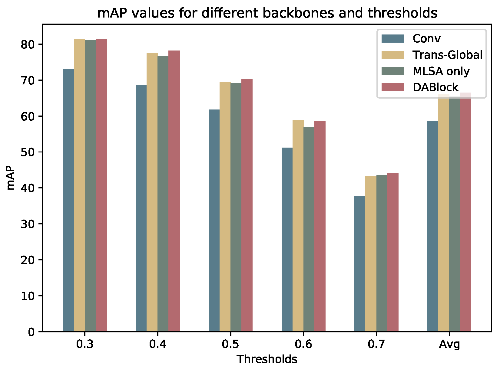
As shown in

Table 3. The ablation study on the effectiveness of MLSA and MA.

Backbone	mAP@0.3	mAP@0.4	mAP@0.5	mAP@0.6	mAP@0.7	mAP@Avg
Conv	73.1	68.5	61.8	51.2	37.8	58.5
Trans-Global	81.3	77.4	69.5	58.8	43.3	66.0
MLSA only	81.0	76.6	69.2	56.9	43.5	65.4
DABlock (adopted)	81.5	78.2	70.3	58.7	44.0	66.5

, DABlock consisting of MLSA and MA outperforms the other structures, achieving an overall average mAP of 66.5%. Figure 3 is the visualization of the effectiveness of MLSA and MA. In addition, convolution has the poorest performance, which demonstrates that Transformer is more suitable for TAL tasks, compared with convolution. In addition, compared with DANet, the global self-attention-based Transformer performs poorer. The plausible reason for this is that global self-attention makes the boundary blurred. When using MLSA only, the feature in time step, t, may discard the connection with the global background. The proposed structure simultaneously focuses on the local changes between adjacent frames and models the global temporal relationship. In addition, DABlock preserves the most informative feature in local clip embedding, which helps to solve the TAL task better.

4.3.2. The Effectiveness of the Number of Projection Layers

We conduct the ablation study to investigate the impact of the number of projection layers, $L_{\mathrm{emd}}$, whose results are presented in

Table 4. The ablation study on the numbers of projections.

${\mathit{L}}_{\mathbf{emd}}$	mAP@0.3	mAP@0.4	mAP@0.5	mAP@0.6	mAP@0.7	mAP@Avg
1	80.3	76.7	68.5	57.6	40.4	64.7
3	80.5	76.4	68.8	57.5	42.7	65.2
4	79.8	75.4	67.2	56.7	42.9	64.4
5	54.5	38.8	21.2	10.0	3.9	25.7
2 (adopted)	81.5	78.2	70.3	58.7	44.0	66.5

. We find an average mAP of 66.5% when the number of projection layers is set to two and observe stable mAP values when the number of layers is less than five. Notably, a poor performance of 25.7% mAP is attained when $L_{\mathrm{emd}}$ is set to five. Through analysis, we conclude that, starting from $L_{\mathrm{emd}}$ = 2, an increase in the number of convolution layers leads to a further transformation of features from local to global representations. Therefore, as the number of layers deepens, it becomes more challenging to process the local features further, resulting in decreased performance.

4.3.3. The Effectiveness of the Adopted Normalization

In this subsection, we investigate the effectiveness of different types of layer normalization on MLSA. Transformer architecture adopts the traditional Post-LN [50], which involves performing the layer normalization operation after multi-headed and residual connections within the Transformer block. Different Post-LN and Pre-LN [50] operations occur before multi-headed attention. Finally, DeepNorm [51] aims to achieve both superior performance and training stability by upscaling the residual connection before conducting the layer normalization process.

The results are presented in

Table 5. The ablation study on Pre-LN, Post-LN, and DeepNorm.

Method	mAP@0.3	mAP@0.4	mAP@0.5	mAP@0.6	mAP@0.7	mAP@Avg
Post-LN	80.4	76.5	68.8	58.1	42.6	65.3
DeepNorm	79.7	75.4	68.3	56.7	43.2	64.7
Pre-LN (adopted)	81.5	78.2	70.3	58.7	44.0	66.5

. It is evident that Pre-LN yields the highest average mAP of 66.5%, followed by Post-LN, which obtains an average mAP of 65.3%, while DeepNorm achieves an average mAP of 64.7%. Therefore, the adopted Pre-LN is reasonable.

4.3.4. The Effectiveness of the Number of Attention Layers

To investigate the effectiveness of the number of DABlock layers, $L_{\mathrm{att}}$, we design five configurations, namely $L_{\mathrm{att}}$ = 3, 4, 5, 6, and 7, whose results are presented in

Table 6. The ablation study on the effectiveness of the numbers of backbone layers.

${\mathit{L}}_{\mathbf{att}}$	mAP@0.3	mAP@0.4	mAP@0.5	mAP@0.6	mAP@0.7	mAP@Avg
3	79.4	75.0	65.8	53.3	37.8	62.2
4	79.9	76.1	68.6	55.4	40.7	64.2
5	81.4	76.3	69.0	56.7	41.5	65.0
7	80.4	76.9	69.3	57.7	43.1	65.5
6 (adopted)	81.5	78.2	70.3	58.7	44.0	66.5

. As $L_{\mathrm{att}}$ increases gradually, the number of downsamplings increases, leading to the representation of higher-level temporal semantic information in the feature maps. The experimental results demonstrate that the model achieves the best performance when $L_{\mathrm{att}}$ is set to 6.

4.3.5. The Effectiveness of Path Aggregation

To investigate the implications of the neck design on model performance, two kinds of feature pyramid structures are tested in this subsection. Specifically, in Design1, we adopt FIP, which does not have path aggregation, i.e., the head is directly connected to its layer. In Design2, we adopt the feature pyramid network [52], which includes path aggregation between layers. Path aggregation refers to the process of combining information from different layers in a neural network. In Design1, where path aggregation is not employed, there is a lack of integration between low-level and high-level semantic information. As a result, certain boundary information remains distinct and is not blurred.

As shown in

Table 7. The ablation study on the effectiveness of path aggregation.

Design	mAP@0.3	mAP@0.4	mAP@0.5	mAP@0.6	mAP@0.7	mAP@Avg
Design2	57.3	40.6	22.5	10.5	4.1	27.0
Design1 (adopted)	81.5	78.2	70.3	58.7	44.0	66.5

, when adopting Design1, the average mAP is 66.4%. In addition, when adopting Design2, the average mAP reduces by 39.5%, compared with Design1. Therefore, the adopted FIP is reasonable.

4.3.6. The Effectiveness of Loss Function

This subsection delves into the impact of loss functions on model performance. Given the regression-based nature of TAL, our analysis focuses on the effect of various regression losses on model efficacy.

The IoU loss [53] regresses the four boundary coordinates of a candidate box as a single entity, leading to efficient and accurate regression with excellent scale invariance. In our model, this two-dimensional loss is compressed into one-dimensional space. The Generalized Intersection over Union (GIoU) loss [54] computes the area of the smallest convex closure, C, between two shapes (like rectangle boxes), A and B, and then calculates the ratio of the area excluding A and B in C to the original area of C. Finally, the original IoU is subtracted from this ratio to obtain the generalized IoU value. The Distance-IoU (DIoU) loss [55] calculates the normalized distance between the center points of two boundary boxes to address the issues of insufficient precision in boundary box regression and slow convergence rate. The Control Distance-IoU (CDIoU) loss [56] mainly contributes to improving the regression accuracy of boundary boxes effectively.

We evaluate the four aforementioned regression losses and the results are presented in

Table 8. The ablation study on the loss function.

Loss	mAP@0.3	mAP@0.4	mAP@0.5	mAP@0.6	mAP@0.7	mAP@Avg
GIoU	81.0	77.6	69.3	57.8	43.0	65.7
CDIoU	80.9	77.2	70.4	58.3	43.5	66.1
DIoU (adopted)	81.5	78.2	70.3	58.7	44.0	66.5

. The experimental results show that, when DIoU is adopted, the average mAP increases 0.4% and 0.8%, respectively, compared with GIoU adopted and CDIoU adopted. Therefore, our design of loss function is reasonable.

4.3.7. The Effectiveness of Warm-Up Epochs

In this subsection, we investigate the impact of the number of warm-up epochs on the overall experimental performance. Warm-up epochs serve as a practical strategy to strike a balance between stability and exploration. They allow the model to improve its performance progressively by effectively utilizing the available training data without comprising convergence or stability. At the beginning of the training, the model is trained with a small learning rate to help it become familiar with the data. Subsequently, the learning rate gradually increases until the set initial learning rate. After a certain number of iterations, the learning rate begins to gradually decrease.

To find out the most suitable number of warm-up epochs, we alter the warm-up epochs between 2 and 8 in our experiment, whose results are presented in

Table 9. The ablation study on the warm-up epochs.

Epochs	mAP@0.3	mAP@0.4	mAP@0.5	mAP@0.6	mAP@0.7	mAP@Avg
2	80.8	77.4	69.8	58.1	42.6	65.7
3	80.9	76.8	69.8	58.2	43.2	65.8
4	81.1	76.6	69.4	58.5	42.8	65.7
6	80.7	76.8	69.8	58.6	43.1	65.8
7	80.8	77.0	69.3	56.8	43.3	65.4
8	80.8	76.5	68.4	57.0	41.9	64.9
5 (adopted)	81.5	78.2	70.3	58.7	44.0	66.5

. The results demonstrate that, when the warm-up epoch is set to 5, the most favorable outcomes are produced. Therefore, our predefined parameter value, i.e., warm-up epoch = 5, is reasonable.

4.4. Visualization

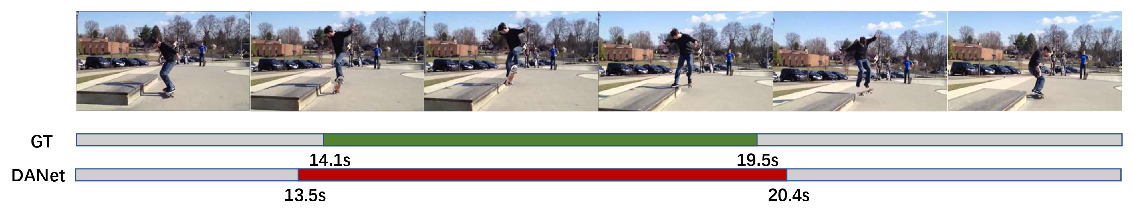
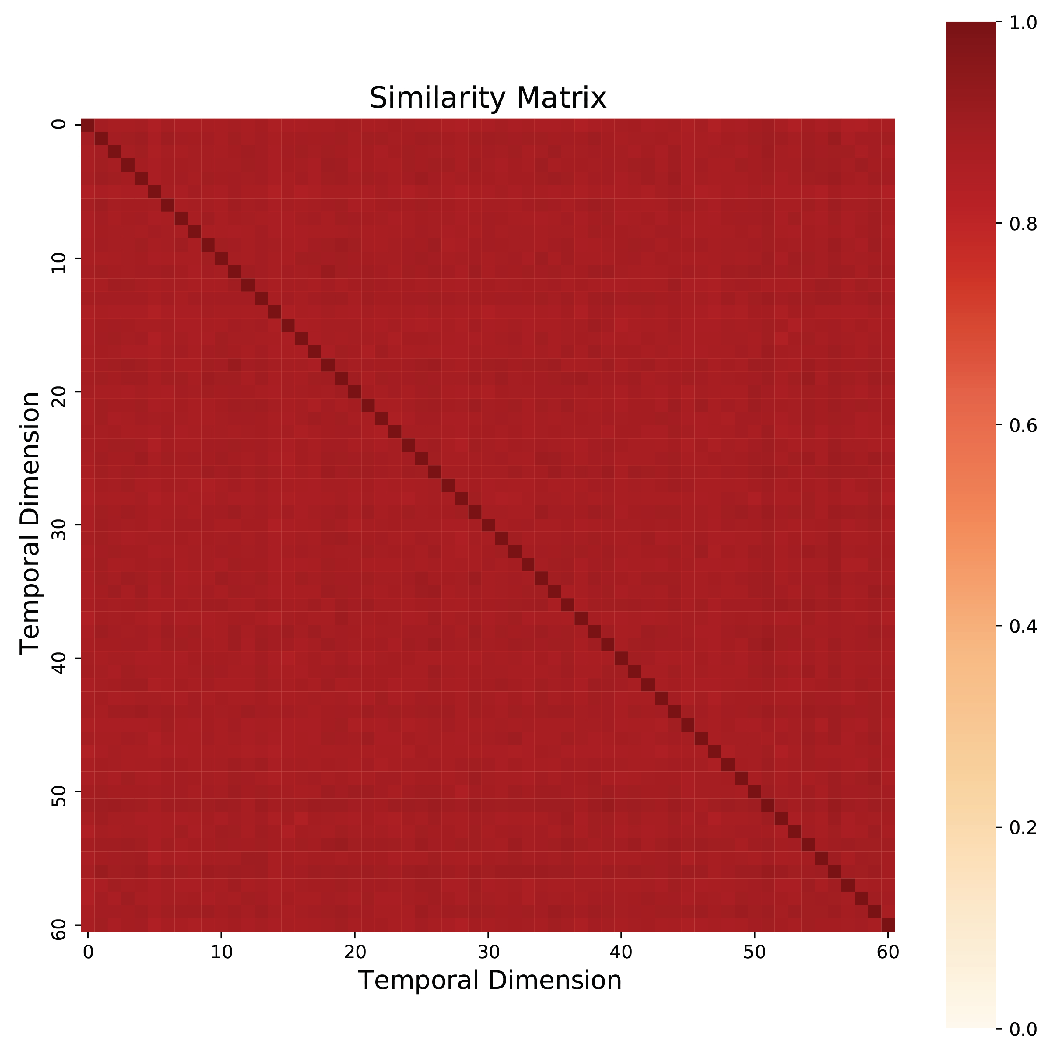
Figure 4 presents the visualization of the proposal generated by our DANet, and compares the predicted results with the ground truth. This action instance is sourced from the THUMOS14 dataset and comprises a skateboarding action of approximately five seconds. It is evident that the temporal offset between our predicted boundary times and ground truth does not exceed one second. Figure 5 illustrates the high degree of similarity between adjacent frames in the video, which underscores the importance of enhancing local sensitivity.

5. Conclusions and Discussion

In this paper, we present our one-stage, anchor-free network model DANet, which leverages a dual-attention mechanism. The core component of DANet is DABlock, which is composed of MLSA and MA. MLSA is utilized for modeling local temporal context. In MA, the max-pooling operation is employed to extract the most significant information from adjacent clip embeddings selectively, while average pooling is used for aggregating global features. Our experimental results on the THUMOS14 and ActivityNet1.3 datasets demonstrate that our approach achieves excellent performance in TAL. While our proposed method has shown good performance in TAL, one of the main limitations is the requirement for fully annotated data, which may not be available in some cases. Further work is to explore weakly supervised learning methods to reduce the dependence on fully annotated data.

References

1. Huang, D.A.; Ramanathan, V.; Mahajan, D.; Torresani, L.; Paluri, M.; Fei-Fei, L.; Niebles, J.C. What makes a video a video: Analyzing temporal information in video understanding models and datasets. In Proceedings of the IEEE Conference on Computer Vision and Pattern Recognition, Salt Lake City, UT, USA, 18–23 June 2018; pp. 7366–7375. [Google Scholar]
2. Wu, C.Y.; Feichtenhofer, C.; Fan, H.; He, K.; Krahenbuhl, P.; Girshick, R. Long-term feature banks for detailed video understanding. In Proceedings of the IEEE/CVF Conference on Computer Vision and Pattern Recognition, Long Beach, CA, USA, 15–20 June 2019; pp. 284–293. [Google Scholar]
3. Lin, J.; Gan, C.; Han, S. Tsm: Temporal shift module for efficient video understanding. In Proceedings of the IEEE/CVF International Conference on Computer Vision, Seoul, South of Korea, 27 October–2 November 2019; pp. 7083–7093. [Google Scholar]
4. Lin, T.; Zhao, X.; Su, H.; Wang, C.; Yang, M. Bsn: Boundary sensitive network for temporal action proposal generation. In Proceedings of the European Conference on Computer Vision, Munich, Germany, 8–14 September 2018; pp. 3–19. [Google Scholar]
5. Lin, C.; Xu, C.; Luo, D.; Wang, Y.; Tai, Y.; Wang, C.; Li, J.; Huang, F.; Fu, Y. Learning salient boundary feature for anchor-free temporal action localization. In Proceedings of the IEEE/CVF Conference on Computer Vision and Pattern Recognition, Nashville, TN, USA, 19–25 June 2021; pp. 3320–3329. [Google Scholar]
6. Liu, X.; Hu, Y.; Bai, S.; Ding, F.; Bai, X.; Torr, P.H. Multi-shot temporal event localization: A benchmark. In Proceedings of the IEEE/CVF Conference on Computer Vision and Pattern Recognition, Nashville, TN, USA, 19–25 June 2021; pp. 12596–12606. [Google Scholar]
7. Lin, T.; Liu, X.; Li, X.; Ding, E.; Wen, S. Bmn: Boundary-matching network for temporal action proposal generation. In Proceedings of the IEEE/CVF International Conference on Computer Vision, Seoul, South of Korea, 27 October–2 November 2019; pp. 3889–3898. [Google Scholar]
8. Long, F.; Yao, T.; Qiu, Z.; Tian, X.; Luo, J.; Mei, T. Gaussian temporal awareness networks for action localization. In Proceedings of the IEEE/CVF Conference on Computer Vision and Pattern Recognition, Long Beach, CA, USA, 15–20 June 2019; pp. 344–353. [Google Scholar]
9. Liu, X.; Wang, Q.; Hu, Y.; Tang, X.; Zhang, S.; Bai, S.; Bai, X. End-to-end temporal action detection with transformer. IEEE Trans. Image Process. 2022, 31, 5427–5441. [Google Scholar] [CrossRef] [PubMed]
10. Zhang, C.L.; Wu, J.; Li, Y. Actionformer: Localizing moments of actions with transformers. In Proceedings of the European Conference on Computer Vision, Glasgow, UK, 23–24 October 2022; pp. 492–510. [Google Scholar]
11. Wu, X.; Han, J.; Wang, D.; Gao, P.; Cui, Q.; Chen, L.; Liang, Y.; Huang, H.; Lee, H.P.; Miao, C.; et al. Incorporating Surprisingly Popular Algorithm and Euclidean distance-based adaptive topology into PSO. Swarm Evol. Comput. 2023, 76, 101222. [Google Scholar] [CrossRef]
12. Wang, L.; Xiao, Y.; Li, J.; Feng, X.; Li, Q.; Yang, J. IIRWR: Internal inclined random walk with restart for lncRNA-Disease association prediction. IEEE Access 2019, 7, 54034–54041. [Google Scholar] [CrossRef]
13. Xiao, Y.; Xiao, Z.; Feng, X.; Chen, Z.; Kuang, L.; Wang, L. A novel computational model for predicting potential LncRNA-disease associations based on both direct and indirect features of LncRNA-disease pairs. BMC Bioinform. 2020, 21, 1–22. [Google Scholar] [CrossRef]
14. Xu, H.; Chen, Z.; Zhang, Y.; Geng, X.; Mi, S.; Yang, Z. Weakly supervised temporal action localization with proxy metric modeling. Front. Comput. Sci. 2023, 17, 172309. [Google Scholar] [CrossRef]
15. Ju, C.; Zheng, K.; Liu, J.; Zhao, P.; Zhang, Y.; Chang, J.; Tian, Q.; Wang, Y. Distilling Vision-Language Pre-training to Collaborate with Weakly-Supervised Temporal Action Localization. In Proceedings of the IEEE/CVF Conference on Computer Vision and Pattern Recognition, Vancouver, BC, Canada, 24–31 January 2023; pp. 14751–14762. [Google Scholar]
16. Xing, Z.; Dai, Q.; Hu, H.; Chen, J.; Wu, Z.; Jiang, Y.G. Svformer: Semi-supervised video transformer for action recognition. In Proceedings of the IEEE/CVF Conference on Computer Vision and Pattern Recognition, Vancouver, BC, Canada, 24–31 January 2023; pp. 18816–18826. [Google Scholar]
17. Qing, Z.; Su, H.; Gan, W.; Wang, D.; Wu, W.; Wang, X.; Qiao, Y.; Yan, J.; Gao, C.; Sang, N. Temporal context aggregation network for temporal action proposal refinement. In Proceedings of the IEEE/CVF Conference on Computer Vision and Pattern Recognition, Nashville, TN, USA, 20–25 June 2021; pp. 485–494. [Google Scholar]
18. Lin, T.; Zhao, X.; Shou, Z. Single shot temporal action detection. In Proceedings of the ACM International Conference on Multimedia, Silicon Valley, CA, USA, 23–27 October 2017; pp. 988–996. [Google Scholar]
19. Vaswani, A.; Shazeer, N.; Parmar, N.; Uszkoreit, J.; Jones, L.; Gomez, A.N.; Kaiser, Ł.; Polosukhin, I. Attention is all you need. In Proceedings of the Advances in Neural Information Processing Systems, Long Beach, CA, USA, 4–9 December 2017; Volume 30. [Google Scholar]
20. Xu, H.; Ma, J.; Yuan, J.; Le, Z.; Liu, W. Rfnet: Unsupervised network for mutually reinforcing multi-modal image registration and fusion. In Proceedings of the IEEE/CVF Conference on Computer Vision and Pattern Recognition, New Orleans, LA, USA, 18–24 June 2022; pp. 19679–19688. [Google Scholar]
21. Boureau, Y.L.; Ponce, J.; LeCun, Y. A theoretical analysis of feature pooling in visual recognition. In Proceedings of the International Conference on Machine Learning, Haifa, Israel, 21–24 June 2010; pp. 111–118. [Google Scholar]
22. Idrees, H.; Zamir, A.R.; Jiang, Y.G.; Gorban, A.; Laptev, I.; Sukthankar, R.; Shah, M. The thumos challenge on action recognition for videos “in the wild”. Comput. Vis. Image Underst. 2017, 155, 1–23. [Google Scholar] [CrossRef] [Green Version]
23. Heilbron, F.C.; Escorcia, V.; Ghanem, B.; Niebles, J.C. Activitynet: A large-scale video benchmark for human activity understanding. In Proceedings of the IEEE/CVF Conference on Computer Vision and Pattern Recognition, Boston, MA, USA, 7–12 June 2015; pp. 961–970. [Google Scholar]
24. Liu, Q.; Wang, Z. Progressive boundary refinement network for temporal action detection. In Proceedings of the AAAI Conference on Artificial Intelligence, New York, NY, USA, 7–12 February 2020; Volume 34, pp. 11612–11619. [Google Scholar]
25. Tan, J.; Tang, J.; Wang, L.; Wu, G. Relaxed transformer decoders for direct action proposal generation. In Proceedings of the IEEE/CVF International Conference on Computer Vision, Montreal, BC, Canada, 10–17 October 2021; pp. 13526–13535. [Google Scholar]
26. Zhu, Z.; Tang, W.; Wang, L.; Zheng, N.; Hua, G. Enriching local and global contexts for temporal action localization. In Proceedings of the IEEE/CVF International Conference on Computer Vision, Montreal, BC, Canada, 10–17 October 2021; pp. 13516–13525. [Google Scholar]
27. Sridhar, D.; Quader, N.; Muralidharan, S.; Li, Y.; Dai, P.; Lu, J. Class semantics-based attention for action detection. In Proceedings of the IEEE/CVF International Conference on Computer Vision, Montreal, BC, Canada, 10–17 October 2021; pp. 13739–13748. [Google Scholar]
28. Xia, H.; Zhan, Y. A survey on temporal action localization. IEEE Access 2020, 8, 70477–70487. [Google Scholar] [CrossRef]
29. Kenton, J.D.M.W.C.; Toutanova, L.K. Bert: Pre-training of deep bidirectional transformers for language understanding. In Proceedings of the Annual Conference of the North American Chapter of the Association for Computational Linguistics: Human Language Technologies, Minneapolis, MN, USA, 2–7 June 2019; Volume 1, p. 2. [Google Scholar]
30. Yang, Z.; Dai, Z.; Yang, Y.; Carbonell, J.; Salakhutdinov, R.R.; Le, Q.V. Xlnet: Generalized autoregressive pretraining for language understanding. In Proceedings of the Advances in Neural Information Processing Systems, Vancouver, BC, Canada, 8–14 December 2019; Volume 32. [Google Scholar]
31. Clark, K.; Luong, M.T.; Le, Q.V.; Manning, C.D. ELECTRA: Pre-training Text Encoders as Discriminators Rather Than Generators. In Proceedings of the International Conference on Learning Representations, Addis Ababa, Ethiopia, 26–30 April 2020. [Google Scholar]
32. Zhang, J.; Zhao, Y.; Saleh, M.; Liu, P. Pegasus: Pre-training with extracted gap-sentences for abstractive summarization. In Proceedings of the International Conference on Machine Learning, Virtual Event, 13–18 July 2020; pp. 11328–11339. [Google Scholar]
33. Dosovitskiy, A.; Beyer, L.; Kolesnikov, A.; Weissenborn, D.; Zhai, X.; Unterthiner, T.; Dehghani, M.; Minderer, M.; Heigold, G.; Gelly, S.; et al. An Image is Worth 16x16 Words: Transformers for Image Recognition at Scale. In Proceedings of the International Conference on Learning Representations, Virtual Event, 3–7 May 2021. [Google Scholar]
34. Liu, Z.; Lin, Y.; Cao, Y.; Hu, H.; Wei, Y.; Zhang, Z.; Lin, S.; Guo, B. Swin transformer: Hierarchical vision transformer using shifted windows. In Proceedings of the IEEE/CVF International Conference on Computer Vision, Montreal, BC, Canada, 10–17 October 2021; pp. 10012–10022. [Google Scholar]
35. Wu, J.; Jiang, Y.; Zhang, W.; Bai, X.; Bai, S. SeqFormer: Sequential Transformer for Video Instance Segmentation. In Proceedings of the European Conference on Computer Vision, Glasgow, UK, 23–24 October 2022; pp. 553–569. [Google Scholar]
36. Sun, C.; Myers, A.; Vondrick, C.; Murphy, K.; Schmid, C. Videobert: A joint model for video and language representation learning. In Proceedings of the IEEE/CVF International Conference on Computer Vision, Seoul, South of Korea, 27 October–2 November 2019; pp. 7464–7473. [Google Scholar]
37. Carreira, J.; Zisserman, A. Quo vadis, action recognition? A new model and the kinetics dataset. In Proceedings of the IEEE/CVF Conference on Computer Vision and Pattern Recognition, Honolulu, HI, USA, 22–25 July 2017; pp. 6299–6308. [Google Scholar]
38. Lin, T.Y.; Goyal, P.; Girshick, R.; He, K.; Dollár, P. Focal loss for dense object detection. In Proceedings of the IEEE International Conference on Computer Vision, Venice, Italy, 22–29 October 2017; pp. 2980–2988. [Google Scholar]
39. Liu, D.; Jiang, T.; Wang, Y. Completeness modeling and context separation for weakly supervised temporal action localization. In Proceedings of the IEEE/CVF Conference on Computer Vision and Pattern Recognition, Long Beach, CA, USA, 15–20 June 2019; pp. 1298–1307. [Google Scholar]
40. Xu, M.; Zhao, C.; Rojas, D.S.; Thabet, A.; Ghanem, B. G-tad: Sub-graph localization for temporal action detection. In Proceedings of the IEEE/CVF Conference on Computer Vision and Pattern Recognition, Seattle, WA, USA, 14–19 June 2020; pp. 10156–10165. [Google Scholar]
41. Zhao, C.; Thabet, A.K.; Ghanem, B. Video self-stitching graph network for temporal action localization. In Proceedings of the IEEE/CVF International Conference on Computer Vision, Montreal, BC, Canada, 10–17 October 2021; pp. 13658–13667. [Google Scholar]
42. Wang, L.; Xiong, Y.; Wang, Z.; Qiao, Y.; Lin, D.; Tang, X.; Van Gool, L. Temporal segment networks: Towards good practices for deep action recognition. In Proceedings of the European Conference on Computer Vision, Amsterdam, The Netherlands, 11–14 October 2016; pp. 20–36. [Google Scholar]
43. Zeng, R.; Huang, W.; Tan, M.; Rong, Y.; Zhao, P.; Huang, J.; Gan, C. Graph convolutional networks for temporal action localization. In Proceedings of the IEEE/CVF International Conference on Computer Vision, Seoul, South of Korea, 27 October–2 November 2019; pp. 7094–7103. [Google Scholar]
44. Lin, C.; Li, J.; Wang, Y.; Tai, Y.; Luo, D.; Cui, Z.; Wang, C.; Li, J.; Huang, F.; Ji, R. Fast learning of temporal action proposal via dense boundary generator. In Proceedings of the AAAI Conference on Artificial Intelligence, New York, NY, USA, 7–12 February 2020; Volume 34, pp. 11499–11506. [Google Scholar]
45. Bai, Y.; Wang, Y.; Tong, Y.; Yang, Y.; Liu, Q.; Liu, J. Boundary content graph neural network for temporal action proposal generation. In Proceedings of the European Conference on Computer Vision, Glasgow, UK, 23–28 August 2020; pp. 121–137. [Google Scholar]
46. Zhao, P.; Xie, L.; Ju, C.; Zhang, Y.; Wang, Y.; Tian, Q. Bottom-up temporal action localization with mutual regularization. In Proceedings of the European conference on Computer Vision, Glasgow, UK, 23–28 August 2020; pp. 539–555. [Google Scholar]
47. Gong, G.; Zheng, L.; Mu, Y. Scale matters: Temporal scale aggregation network for precise action localization in untrimmed videos. In Proceedings of the IEEE International Conference on Multimedia and Expo, London, UK, 6–10 July 2020; pp. 1–6. [Google Scholar]
48. Qiu, Z.; Yao, T.; Mei, T. Learning spatio-temporal representation with pseudo-3d residual networks. In Proceedings of the IEEE International Conference on Computer Vision, Venice, Italy, 22–29 October 2017; pp. 5533–5541. [Google Scholar]
49. Yang, L.; Peng, H.; Zhang, D.; Fu, J.; Han, J. Revisiting anchor mechanisms for temporal action localization. IEEE Trans. Image Process. 2020, 29, 8535–8548. [Google Scholar] [CrossRef]
50. Xiong, R.; Yang, Y.; He, D.; Zheng, K.; Zheng, S.; Xing, C.; Zhang, H.; Lan, Y.; Wang, L.; Liu, T. On layer normalization in the transformer architecture. In Proceedings of the International Conference on Machine Learning, Virtual, 13–18 July 2020; pp. 10524–10533. [Google Scholar]
51. Wang, H.; Ma, S.; Dong, L.; Huang, S.; Zhang, D.; Wei, F. DeepNet: Scaling Transformers to 1000 Layers. arXiv 2022, arXiv:2203.00555. [Google Scholar]
52. Lin, T.Y.; Dollár, P.; Girshick, R.; He, K.; Hariharan, B.; Belongie, S. Feature pyramid networks for object detection. In Proceedings of the IEEE/CVF Conference on Computer Vision and Pattern Recognition, Honolulu, HI, USA, 21–26 July 2017; pp. 2117–2125. [Google Scholar]
53. Yu, J.; Jiang, Y.; Wang, Z.; Cao, Z.; Huang, T. Unitbox: An advanced object detection network. In Proceedings of the ACM International Conference on Multimedia, Amsterdam, The Netherlands, 15–19 October 2016; pp. 516–520. [Google Scholar]
54. Rezatofighi, H.; Tsoi, N.; Gwak, J.; Sadeghian, A.; Reid, I.; Savarese, S. Generalized intersection over union: A metric and a loss for bounding box regression. In Proceedings of the IEEE/CVF Conference on Computer Vision and Pattern Recognition, Long Beach, CA, USA, 15–20 June 2019; pp. 658–666. [Google Scholar]
55. Zheng, Z.; Wang, P.; Liu, W.; Li, J.; Ye, R.; Ren, D. Distance-IoU loss: Faster and better learning for bounding box regression. In Proceedings of the AAAI Conference on Artificial Intelligence, New York, NY, USA, 7–12 February 2020; Volume 34, pp. 12993–13000. [Google Scholar]
56. Dong, C.; Duoqian, M. Control Distance IoU and Control Distance IoU Loss for Better Bounding Box Regression. Pattern Recognit. 2023, 137, 109256. [Google Scholar] [CrossRef]
Figure 1. Overview of the proposed DANet, comprising feature extractor, backbone, neck, and head.
Applsci 13 07176 g001
Figure 2. Illustration of the structure of the proposed MA. We use MA to preserve critical local features by employing max-pooling, and aggregate global feature information via average-pooling, denoted as Avg Pooling. Attention weights spanning both channel and temporal dimensions are generated to aid in this process. These weight variables are computed based on the importance of different feature elements and are crucial for improving the model’s representation capability.
Applsci 13 07176 g002
Figure 3. Visualization of the effectiveness of MLSA and MA.
Applsci 13 07176 g003
Figure 4. Illustration of the results of our experiment, where the video clip is sourced from THUMOS14 and comprises a complete skateboarding action. The green region below denotes the ground truth, while the red region denotes the proposals predicted by our model.
Applsci 13 07176 g004
Figure 5. In a video, adjacent frames are typically highly similar. This figure presents the correlation matrix of adjacent frames, with stronger correlation indicated by darker colors and weaker correlation indicated by lighter colors.
Applsci 13 07176 g005