A New Defect Diagnosis Method for Wire Rope Based on CNN-Transformer and Transfer Learning

Abstract

Accurate wire rope defect diagnosis is crucial for the health of whole machinery systems in various industries and practical applications. Although the loss of metallic cross-sectional area signals is the most widely used method in non-destructive wire rope evaluation methods, the weakness and scarcity of defect signals lead to poor diagnostic performance, especially in diverse conditions or those with noise interference. Thus, a new wire rope defect diagnosis method is proposed in this study. First, empirical mode decomposition and isolation forest methods are applied to eliminate noise signals and to locate the defects. Second, a convolution neural network and transformer encoder are used to design a new wire rope defect diagnosis network for the improvement of the feature extraction ability. Third, transfer learning architecture is established based on gray feature images to fine-tune the pre-trained model using a small target domain dataset. Finally, comparison experiments and a visualization analysis are conducted to verify the effectiveness of the proposed methods. The results demonstrate that the presented model can improve the performance of the wire rope defect diagnosis method under cross-domain conditions. Additionally, the transfer feasibility of transfer learning architecture is discussed for future practical applications.

1. Introduction

Wire rope is widely used in many fields, such as coal mine hoists, bridge construction, escalators, cranes, and ocean platforms for natural gas extraction [1]. Due to the harsh working conditions in these fields, various defects inevitably occur during its whole life cycle [2]. Furthermore, the condition of wire rope is of great importance for the stable operation of machines and the safety of human lives [3]. 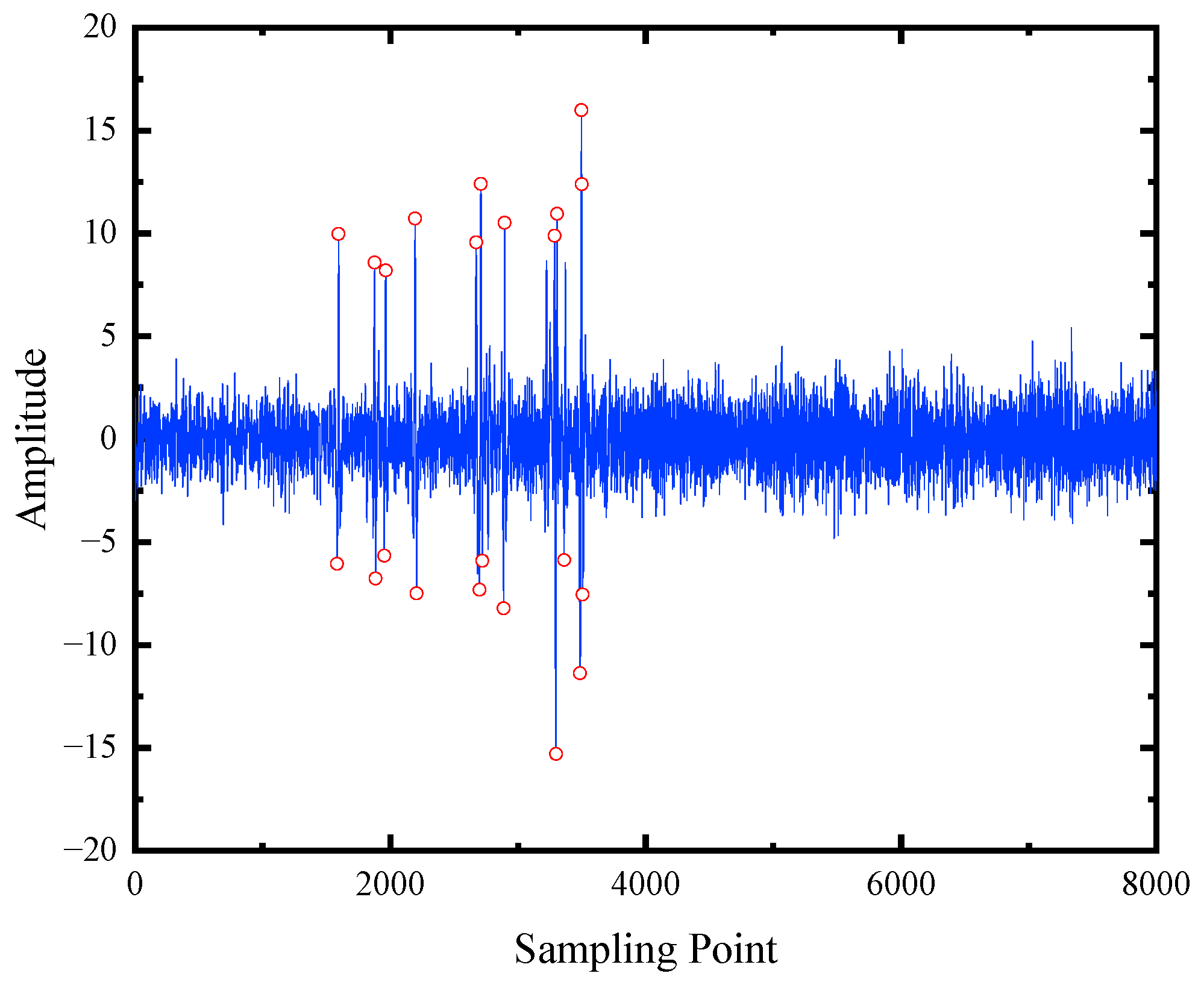Magnetic flux leakage (MFL) [4] is one of the most prevalent non-destructive electromagnetic testing methods used in practical applications, where the loss of metallic cross-sectional area (LMA) defects can be detected both effectively and rapidly. However, the analysis of this method is difficult when LMA signals are combined with different noises that are generated by electromagnetic interference, detection speeds, the pole tip effect, or movement friction [5]. Hence, the accurate defect diagnosis of wire rope is necessary and meaningful for machines to present greater reliability. In addition, reducing maintenance costs is another benefit that arises from wire rope defect diagnosis research.

In recent years, breakthroughs in image processing methods have provided increased directions for wire rope signal processing and feature extraction techniques. Based on the matrix reconstruction method and the fact that two-dimensional (2D) imaging provides a better platform for feature extraction in comparison to standard one-dimensional (1D) signals, numerous detection algorithms have been proposed and demonstrated in the literature [6,7,8]. To improve the robustness and accuracy outcomes of wire rope defect inspections, Liu et al. proposed some novel methods to complete quantitative defect recognition practices, including a reshaped sine function, wavelet function, and grid entropy. Finally, the feasibility of the presented methods is verified through case studies that are conducted under different working conditions [9]. In a recent study, Li et al. presented the establishment of MFL gray images and combined a kernel extreme learning machine with a compressed sensing wavelet to inhibit noise interference and improve the accuracy of wire rope defect recognition results [10]. From the perspective of solving noise interference issues, Liu et al. designed a new signal processing method based on notch filtering and wavelet denoising for successfully detecting defect signals in the MFL data, which was demonstrated by a series of experiments and processing results [11].

It is well known that deep learning and neural networks have achieved great success in numerous fields, such as image classification [12,13], object detection [14,15], and natural language processing [16]. These new approaches can automatically extract features instead of depending on prior knowledge. Furthermore, the advantage of deep learning networks is their better generalization and robustness. Based on machine learning techniques, some methods were proposed in the literature and demonstrated to be effective for various defect diagnosis tasks in mechanical industries, such as drag machines, gearbox diagnosis, motor fault detection, and rotor-bearing systems [17]. Eren et al. used raw sensor signal as an input to establish a compact, adaptive, 1D convolution neural network (CNN) classifier for bearing fault diagnosis without any pre-determined feature extraction or feature selection methods, and the effectiveness and feasibility of the proposed method were validated by comparing the results with other competing intelligent fault diagnosis algorithms [18]. Based on an artificial neural network, Sahu et al. applied a multilayer perceptron in a drag system to improve the sensitivity of their fault symptom identification and demonstrated the effectiveness of minimizing the failure frequency and maintenance costs [19]. To address the difficulties of acquiring labeled samples, He et al. proposed a new framework based on small-labeled infrared thermal images and an enhanced CNN for monitoring the vibration of a rotor-bearing system fault diagnosis, which was demonstrated to be superior to the mainstream methods used to date [20]. Some studies also focused on transfer learning (TL) methods to minimize the discrepancy between two datasets of working conditions, which aimed to avoid long time-consuming training and insufficiently labeled data. Wang et al. designed a novel fault diagnosis network that was constructed by a deformable CNN, deep long short-term memory, and dense layers based on transfer learning strategies, and their cross-domain experiments demonstrated its effectiveness in identifying the fault types of bearings in new conditions [21]. Ma et al. proposed a transfer diagnosis framework based on an improved domain adaptation algorithm, and their related comparison of the experimental results demonstrated the applicability and practicability of the proposed method compared with other existing state-of-the-art (SOTA) algorithms [22]. Some studies also used machine learning methods to detect wire rope defects, such as neural networks, support vector machine (SVM) [23], and multi-channel signal fusion, to improve the performance of defect detection activities under conditions of vigorous movement and strand noise [24]. Undoubtedly, the mentioned studies yielded positive effects from different aspects; however, for cross-domain working conditions and those with noise interference, further improvements and increased robustness can be achieved in wire rope defect diagnosis.

Aiming to improve wire rope defect diagnosis performance under diverse working conditions from LMA signals, a new CNN-transformer network and TL architecture are proposed in this paper to improve the defect detection accuracy. The main contributions and novelties of this paper are the following:

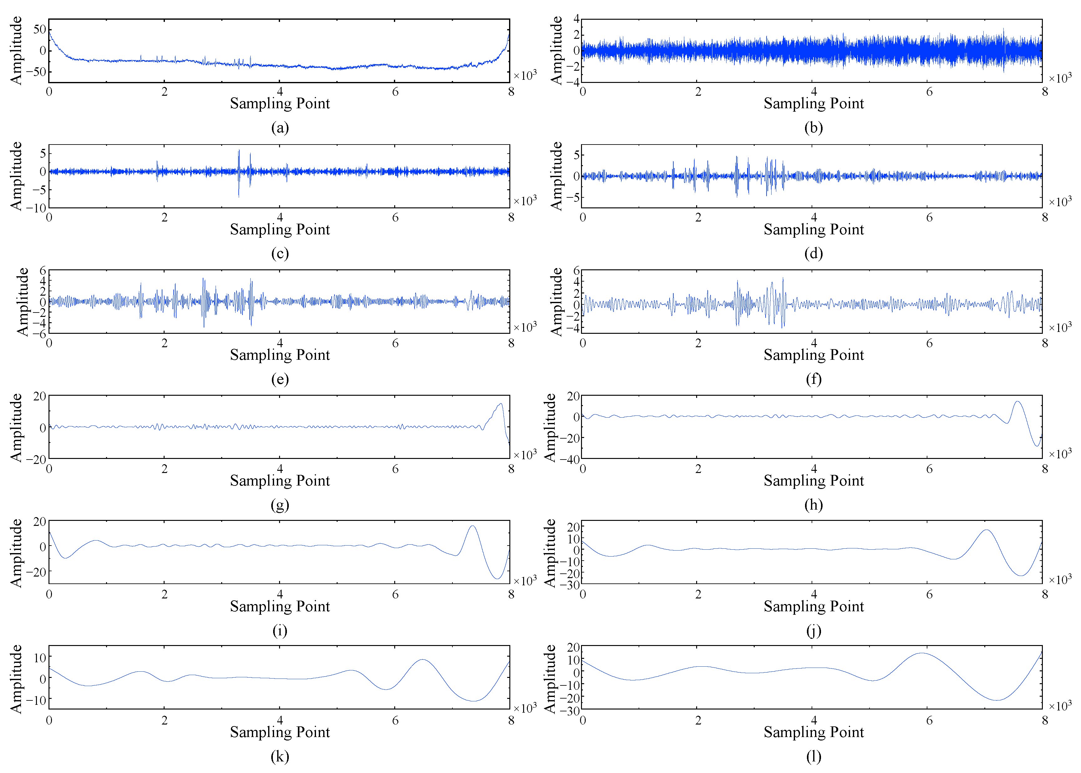
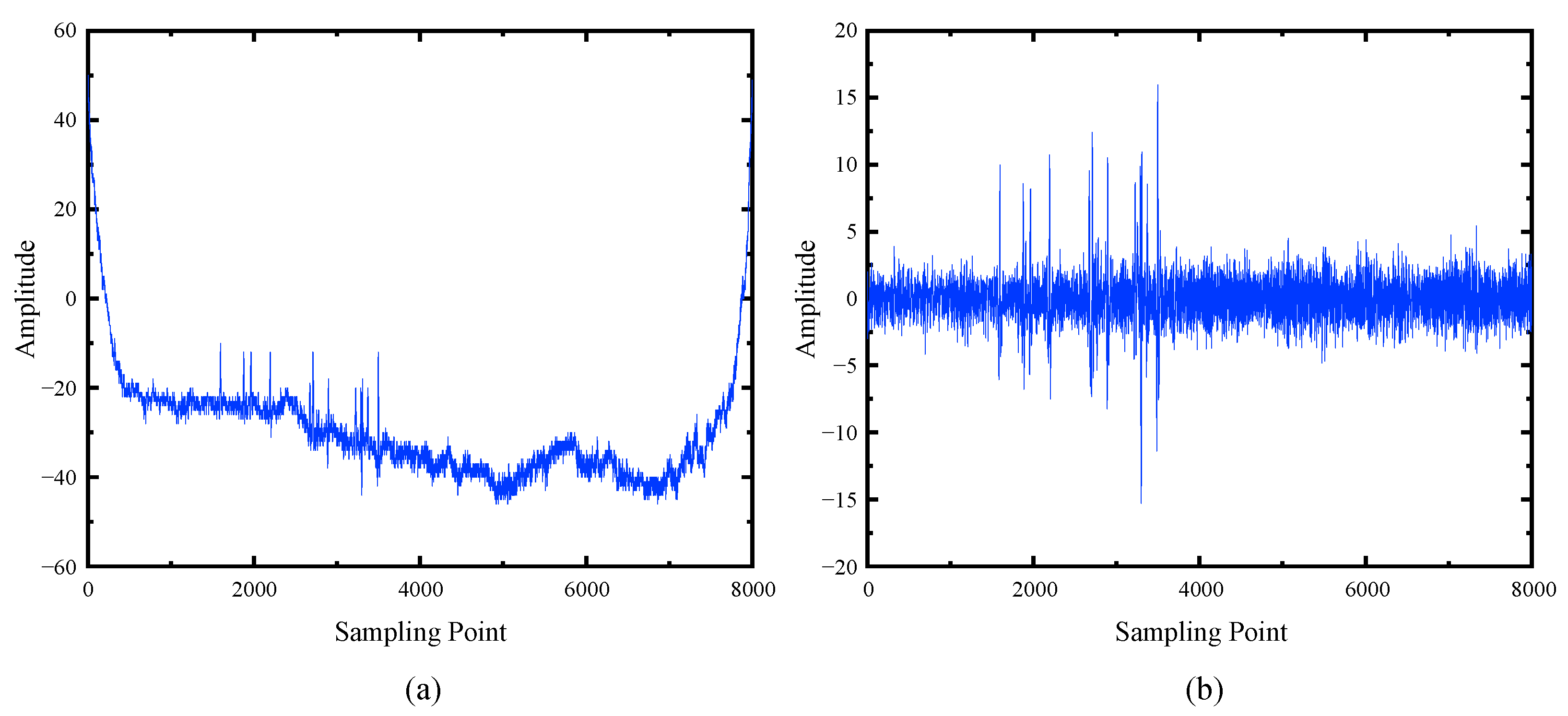
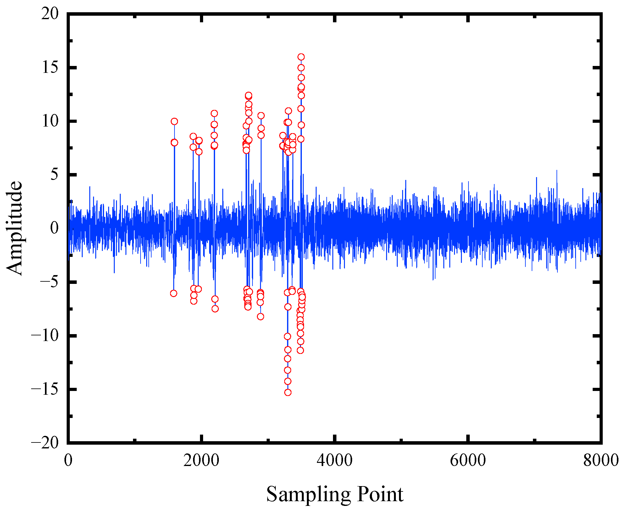
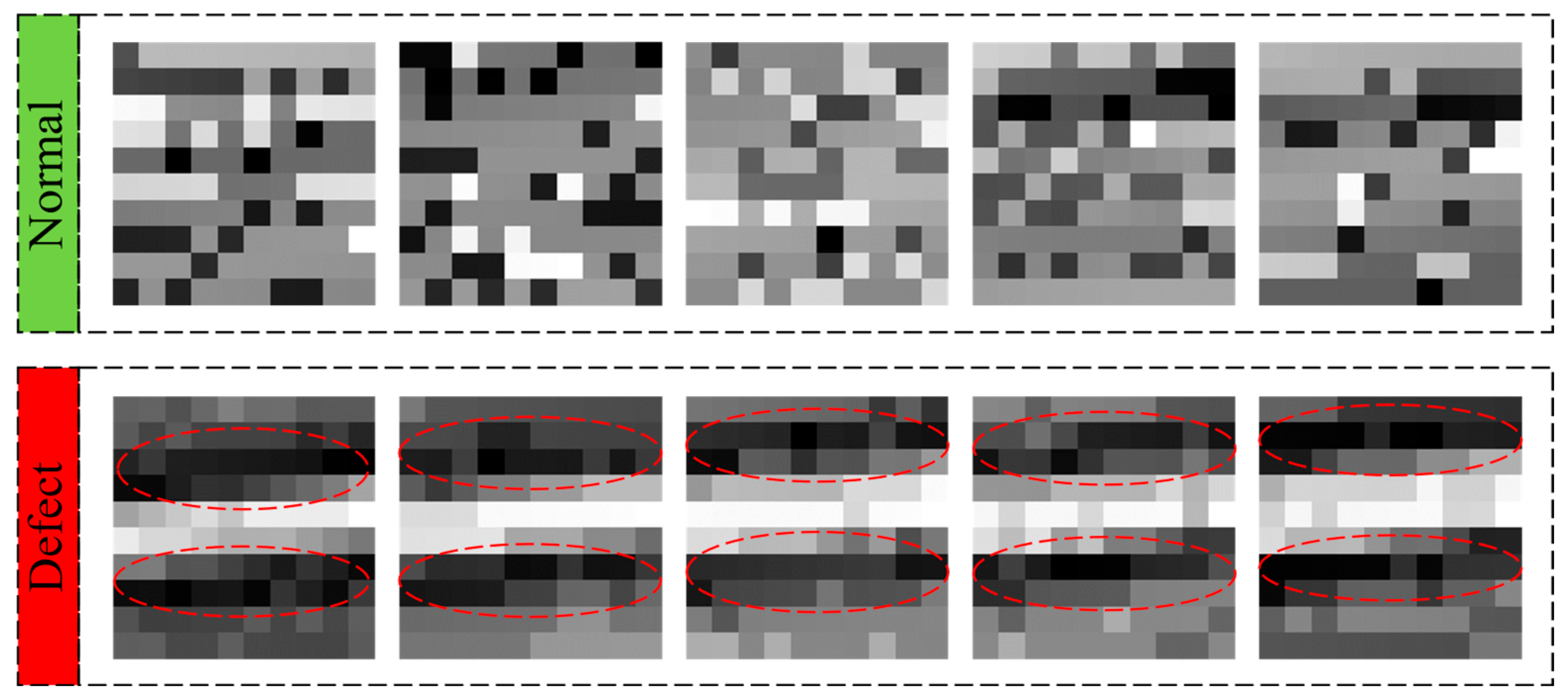
(1) A data preprocessing method based on empirical mode decomposition (EMD) is presented to eliminate the adverse interference of various noises. Two-dimensional gray images are processed through matrix reconstruction and data augmentation methods for the preparation of a wire rope training dataset.

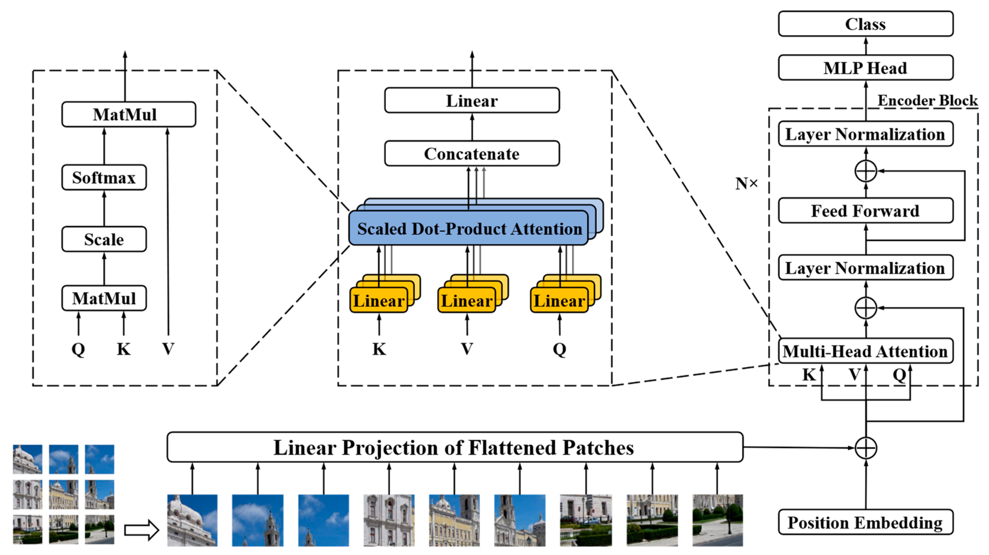
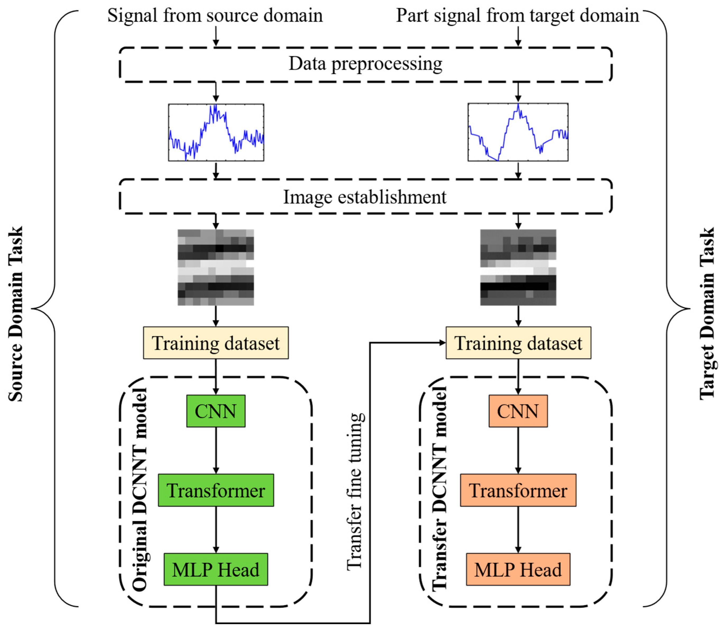
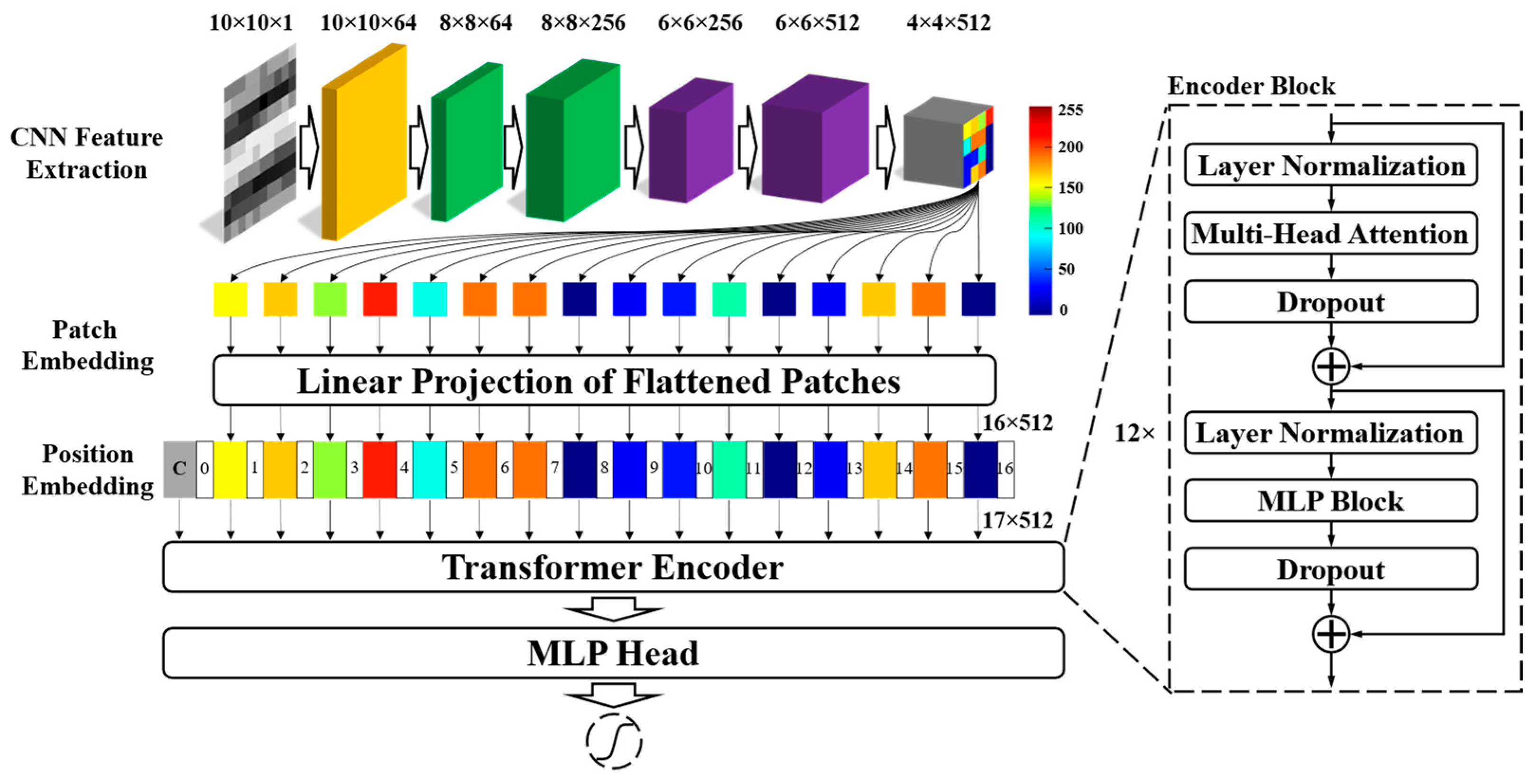
(2) Through the combination of CNN and a transformer, a novel wire rope defect diagnosis network is proposed and named DCNNT, where the defect information can be effectively extracted, computational complexities are reduced, and forward efficiency is improved.

(3) Unlike the existing approaches in the literature, this paper focuses on solving the issues of domain adaptation and wire rope defect data that are insufficient. A new TL architecture is established based on TL techniques and the proposed DCNNT.

(4) The effectiveness of the proposed DCNNT and domain adaptation ability of the TL architecture are verified through different comparison experiments with several general and SOTA methods, where the proposed model can balance detection accuracy, forward latency, and network parameters.

This paper is organized as follows: The related study is reviewed in Section 2. Section 3 is the methodology of the proposed methods, including original data preprocessing based on EMD, feature image processing based on matrix reconstruction, TL architecture establishment, and DCNNT network structure. In Section 4, case studies are conducted through comparison experiments and visualization analysis. Conclusions are presented in Section 5.

2. Related Works

2.1. CNN Theory

With the development of machine vision, the effectiveness of the CNN has been proven in many studies, especially those addressing feature extraction and processing speed. Usually, convolution, pooling, and fully connected layers are the main components of the CNN operation. Through CNN, different feature maps can be obtained and the number of channels is determined by the kernel size. This process can be defined as:

$$x_i^l=f\left({\displaystyle \sum _{j=1}^n{W}_{i,j}^l\times x_j^{l-1}+b_i^l}\right)$$

(1)

where $x_i^l$ is the $i\mathrm{th}$ output feature map of the $l\mathrm{th}$ layer. $x_i^{l-1}$ denotes the $j\mathrm{th}$ input feature map of the $\left(l-1\right)\mathrm{th}$ layer, $W_{i,j}^l$ is the weight matrix between the $i\mathrm{th}$ feature map of the $l\mathrm{th}$ layer and $j\mathrm{th}$ is the feature map of the $\left(l-1\right)\mathrm{th}$ layer, $b_i^l$ is the bias of the $i\mathrm{th}$ output feature map in the $l\mathrm{th}$ layer, and $f\left(·\right)$ is the activation function that is required to increase the nonlinearity of the model. The ReLU [25] function has excellent performance and was adopted in this study. The definition is:

$$f(x)=\max (0,x)$$

(2)

The pooling layers can reduce the parameters of the whole network and ensure the translation is invariant during the prediction process. The common methods used include max pooling, mean pooling, and stochastic pooling. The fully connected layers are often used at the end of the network to complete the dimension change step. In this process, the feature maps are flattened into 1D vectors as the input of fully connected layers. The operation can be defined as:

$$y^l=f\left(w^l{x}^{l-1}+b^l\right)$$

(3)

where $y^l$ is the output of the $l\mathrm{th}$ fully connected layer, $x^{l-1}$ is the input vector from the $\left(l-1\right)\mathrm{th}$ layer, $w^l$ is the weight vector of the nodes between the $l\mathrm{th}$ and $\left(l-1\right)\mathrm{th}$ layers, and $b^l$ is the bias.

2.2. Vision Transformer (ViT)

In the year 2020, Dosovitskiy et al. applied the transformer [26] to image classification tasks directly and termed the proposed method as ViT [27]. Based on the attention mechanism, ViT feeds the sequences of image patches directly to the standard transformer network and produces good detection results. As shown in Figure 1, ViT only uses the transformer encoder which includes residual connectors, layer normalization, and the multi-head attention mechanism. Following the patch and position embedding stages, the 1D sequence is fed into the encoder blocks. The multi-head attention mechanism is the most important module and has the role of discovering the relationship between different elements from other tokens in the sequence. Similar to the standard transformer, three trainable weight matrices exist ($W^q$, $W^k$, $W^v$) which are responsible for query, key, and value projections, respectively. During training using a certain batch size, the input can be expressed as matrix $X$. Consequently, $Q=X{W}^q$, $K=X{W}^k$, and $V=X{W}^v$ can be obtained as the inputs of the self-attention mechanism. The dot-product attention mechanism is depicted as the left dashed box and the operation of the single-head attention can be defined as:

$$Attention{(Q,K,V)}_h=Softmax(Q_h{K}_h^T/\sqrt{d})V_h$$

(4)

where the attention matrix $A=Q{K}^T$ is responsible for the learning alignment scores between tokens in the sequence, and $d$ is a scaling factor used to prevent excessive output in $A$. As shown in the middle block, $MultiHead\left(Q,K,V\right)=W^o·Concat\left(A_1,A_2,...,A_H\right)$ can be obtained through concatenated operation and linear projection ($W^o$). Similarly, by stacking the encoder blocks on top of one another, a transformer encoder can be established. Finally, the multi-layer perceptron (MLP) head is used for classification tasks.

2.3. Transfer Learning

Transfer learning (TL) is an excellent technique used for machine learning practices and is often used to rapidly improve detection accuracy between different working conditions. The purpose of TL is to find out the commonality between source and target domains following different distributions [28,29]. The definition of TL is described as training models in the source domain ($D_s=\left\{X_s,P\left(X_s\right)\right\}$) and complete source task ($T_s=\left\{Y_s,f_s\right\}$), then the fine-tuning model in the target domain ($D_t=\left\{X_t,P\left(X_t\right)\right\}$) and complete target task ($T_t=\left\{Y_t,f_t\right\}$), where $X=\left\{x|x_i\in X,i=\mathrm{1,2},...,n\right\}$ is the feature space, $P$ denotes the probability distribution, and $f$ is the learned function of the model. In summary, TL helps to reduce the overall training time and does not require changing the structure of the model. Moreover, model training only requires a few labeled datasets obtained from the target domain.

3. Methodology

3.1. Data Preprocessing

Non-destructive testing technology based on MFL is widely used in the research of wire rope diagnosis activity. Due to harsh working conditions and different structures of wire rope, such as aggressive movement, electromagnetic interference, the pole tip effect, and movement friction, MFL signals are inevitably mixed with various noises that have an adverse impact on the defect diagnosis result. All of these factors contribute to the difficulty of extracting useful features from the original signals. Therefore, it is necessary to conduct the data preprocessing step, prior to further operations of feature extraction and defect detection.

As one typical MFL signal commonly used in practical applications, the LMA signal was selected to analyze the condition of the wire rope. Furthermore, a large number of studies have proved the validity of the EMD [30] method for processing nonlinear or nonstationary signals [31]. In this paper, the EMD method was used to preprocess the original LMA signals and realize the function of denoising. As described in Equation (5), the original signal ($x\left(t\right)$) can be divided into several intrinsic mode function (IMF) signals ($s\left(t\right)$) and one residual signal ($r\left(t\right)$). According to the principle of EMD, each IMF signal reflects different frequency components and signal features. By recombining the useful IMFs, the purpose of eliminating noise signals can be achieved. Specifically, the constraints on the IMF signal are as follows:

• For each IMF signal, the number of extreme points should be equivalent to zero crossing points, or the difference cannot be greater than one.
• The upper envelope formed by maxima and the lower envelope formed by minima should be symmetrical and the average values must be zero at any moment.

$$x(t)={\displaystyle \sum _{i=1}^n{S}_i(t)+r(t)}$$

(5)

According to the EMD method, ten different IMF signals and one residual signal can be obtained, these are presented in Figure 2. When these IMF signals are observed and compared to the original LMA signal, it can be determined that most of these noise-interference signals can be divided into different IMFs, which can be obviously separated from the useful information. Thus, the signals presented in Figure 2, from (g) to (l), can be understood as noise because of the pole tip effect or strand wave structure, which should be removed. Similarly, the signals, from (b) to (f), containing defect information should be reconstructed to complete the data preprocess and feature refinement stages. After EMD decomposition and reconstruction, the refined signals are presented in Figure 3b, which exhibits improved clarity and stability results, and the defect signal features are more obvious. This is beneficial to further feature extraction and defect diagnosis steps.

3.2. Image Establishment

3.2.1. Defect Location

For the establishment of normal and defect feature images, defect location is necessary and crucial to further model training outcomes. According to the characteristics of the LMA signals, the defect samples are small when compared with the normal components, and their fluctuations and changes are obvious. Therefore, an excellent anomaly detection algorithm, isolation forest (iForest), was used in this study to complete defect pre-locations from the numerous normal data. The detail of iForest can be observed in reference [32]. The detection results are different as the hyper-parameters change. According to the professional’s prior knowledge, the number of iterations, isolation trees, and sub-sample heights were set as 10, 100, and 256, respectively. Meantime, the detection threshold was 99.5%, that is, 0.05% of abnormal components could be detected. Although the defect signals indicated by the red spot can be clearly located, as shown in Figure 4, multiple data for each defect location still exist, which need to be processed further to meet the requirements of data extension and image processing.

Although the iForest method can effectively detect the defect signals, an additional processing step is required to obtain the single maxima and minima values for each defect sample. Local extremum is a common and simple algorithm used in signal processing methods, which can be used as a filter for data optimization. The window size of the local extremum filter is an important parameter and it must be adjusted according to real applications. In this study, the window size was 100 and the final output results were acceptable. As shown in Figure 5, every result (red dot) can clearly locate each defect sample, which provides a foundation for feature image establishment.

3.2.2. Image Processing

First, data extension and segmentation steps were conducted. The purpose of the data extension step is to provide an adequate amount of data for feature image processing and a simple explanation of this step is the use of the detected defect extreme points as the axial center and the addition of certain data points at both sides. The feature image is established at a size of $10\times 10$ and the data extension numbers located on the left and right sides are set to 49 and 50, respectively. Consequently, 1D defect signals can be obtained and the remaining data are segmented at the same lengths. Namely, there are 100 signal points in each sample, whether they are normal or defect data. Specifically, the length of the data should be adjusted according to the real application since it can affect the diagnosis resolution during an online diagnosis.

Second, 1D signals are recreated into 2D feature images through the matrix reconstruction method. Moreover, all the data presented in each sample should be max–min normalized and mapped to 0–255 using Equation (6). Where, $X\left(i\right)$ is the $i^{th}$ sample of the 1D signals and $X{\left(i\right)}_{max}$ and $X{\left(i\right)}_{min}$ are the maximum and minimum values of $X\left(i\right)$.

$$S(i)=\frac{X{(i)}_{\max }-X(i)}{X{(i)}_{\max }-X{(i)}_{\min }}\times 255$$

(6)

Then, the matrix reconstruction method is employed to obtain the $10\times 10$ matrix, and the element of the transformed matrix is used as the pixel of a gray image, a simple feature image ($M$) can be established using Equation (7):

$$M=\tau \left[S{(i)}_{L\times 1}\right]$$

(7)

where function $\tau [·]$ is an operation from 1D signals $S\left(i\right)$, which contain $L$ data points for the 2D matrix, and the process can be defined as Equation (8):

$$\tau \left[S(i)\right]:\left[s(1),s(2),s(3),\cdots ,s(L)\right]\to \left[\begin{array}{cccc}{P}_{11}& P_{12}& \cdots & P_{1n}\\ ⋮& ⋮& & ⋮\\ P_{m1}& P_{m2}& \cdots & P_{mn}\end{array}\right]$$

(8)

Particularly, $L$ should present a square root if the final image is transformed into a square matrix. Here, $L={mn=k}^2$, where $k$ is the order of the right matrix and defined as 10 in this paper. During the process of matrix reconstruction, the relationship between each datum of $S\left(i\right)$ and the matrix can be calculated by Equation (9), where $m$ and $n$ are the row and column indexes of the final matrix value, respectively.

$$P_{mn}=s\left(k\times (m-1)+n\right)$$

(9)

According to the algorithm presented in

Table 1. Algorithm of feature image establishment.

Step	Description
1	Original LMA signal preparation
2	Data preprocessing based on the EMD method
3	Defect location based on the isolation forest and local extremum method
4	Data extension and segmentation
5	Normal and defect feature image generation based on matrix reconstruction
6	End

, the normal and defect feature images can be obtained and are presented in Figure 6. Obviously, image expression is more intuitive and distinguished when compared with the 1D original LMA signals. Moreover, those characteristics in different types of images are clear and distinguishable. As indicated by the red dotted line, it can be observed that the wire rope defect information changes into black-and-white cross stripes that are caused by the intense fluctuations in the defect LMA signals. Furthermore, cross stripes exist in all defect images; this is beneficial for the improvement of robustness and consistency outcomes achieved during the defect detection process. Unlike the defect images, normal images are characterized by random noise points instead of cross stripes because MFL signals can only be captured at defect locations.

3.3. Transfer Learning Architecture

As shown in Figure 7, the designed TL architecture for wire rope defect diagnosis mainly consists of four steps and two tasks: data preprocessing, image establishment, DCNNT model pre-training and fine-tuning, and source domain and target domain tasks. The details of the DCNNT are described in Section 3.4.

TL architecture focuses on model pre-training and fine-tuning stages that are necessary and crucial for successful domain adaptation results. The dataset of feature images between source and target domains presents different data distributions and the number of the latter is usually scarcer in practical implementations due to real-life limitations. The definition of the source domain task is pre-training performed using high numbers of images obtained from the source domain with all categories (normal and defect); then, an original DCNNT model can be created (green highlight). Consequently, the target domain task is the fine-tuning of the internal parameters of the trained model using a part of the target domain dataset to create a better transfer DCNNT model (orange highlight). The purpose of the proposed TL architecture is to use a small target domain dataset to rapidly create an effective model, instead of using time-consuming retraining methods. According to the TL strategy, the unfreeze training from lower to higher layers was implemented in this study. The relevant details can be observed in reference [33].

3.4. DCNNT Model

The intuition of the DCNNT model lies in ViT and the purpose of reducing computational complexity, making it possible to train and predict using a common personal computer while improving the prediction performance. As depicted in Figure 8, the DCNNT model is also a deep learning network based on the CNN and transformer.

The CNN module is the initial step and its main function is to pre-extract features and reshape $10\times 10\times 1$ wire rope feature images into a 1D feature sequence to reduce the computational complexity produced during the latter transformer module. The CNN is designed as the backbone network and simply consists of standard convolution, max pooling, and batch normalization stages. As summarized in

Table 2. CNN backbone network architecture for DCNNT.

Layers	Filter Shape	Output Size
Conv-1	3 × 3 conv, stride 1, padding 1	$10\times 10\times 64$
Normal-1/Pooling-1	3 × 3 conv, stride 1, padding 0	$8\times 8\times 64$
Conv-2	3 × 3 conv, stride 1, padding 1	$8\times 8\times 256$
Normal-2/Pooling-2	3 × 3 conv, stride 1, padding 0	$6\times 6\times 256$
Conv-3	3 × 3 conv, stride 1, padding 1	$6\times 6\times 512$
Normal-3/Pooling-3	3 × 3 conv, stride 1, padding 0	$4\times 4\times 512$

Conv-1 denotes the first layer of the convolution operation. Similarly, normal and pooling are the normalization and max pooling layers.

, three operation blocks exist, and each block has the same configurations in filter shape. Following the application of the CNN, the size of the feature maps is adjusted from $10\times 10$ to $4\times 4$ and the number of channels is increased to 512.

Pseudo-color is used to visualize the entire data flow process and the color bar is a supplement for reflecting the data values. In the patch embedding stage, we flattened the $4\times 4\times 512$ feature maps to $16\times 512$, and each patch become a 512 vector with a trainable linear projection. Similar to the standard transformer, a learnable class token (gray patch) was added to be responsible for the classification task. Meanwhile, standard learnable 1D embeddings were used to add position information. Then, the data flow shape was $17\times 512$ and the resulting sequence of embedding vectors was fed to the transformer encoder. The dotted box diagram represents the structure of a single encoder block.

Table 3. The parameters of DCNNT encoder variants.

Patch Size	Encoder Block	Hidden Size	MLP Size	Heads
$4\times 4$	12	512	2048	8

presents the details of DCNNT encoder variants, twelve encoder blocks were stacked to establish a transformer encoder. The number of multi-head attention networks was set to eight to achieve computationally economic results. The MLP head is a simple linear layer that has the same neural nodes as the diagnosis class.

4. Case Studies

4.1. Wire Rope Dataset

The dataset used in this paper was collected using a wire rope LMA signal detector, as illustrated in Figure 9a. The main type of defect was a broken wire rope which is indicated in Figure 9b,c. Under different working conditions, the LMA signals of four wire ropes used in the mine hoist were obtained and divided into groups A, B, C, and D, respectively. According to the image establishment method mentioned in Section 3.2, the number of wire rope feature images is presented in

Table 4. Numbers of normal and defect feature images in the wire rope dataset.

	A	B	C	D
Normal	1371	2660	2593	2572
Original Defect	27	59	85	98
Augmentation Defect	297	649	935	1078

. It can clearly be observed that the highest ratio between the number of normal and defect signals is approximately 50:1. This serious imbalance dataset has a negative effect on source domain training and prediction tasks [34]. Therefore, sample augmentation for the defect images was necessary, and the augmentation algorithm steps are depicted in

Table 5. Algorithm of defect sample augmentation.

Step	Description
1	Original LMA signal preparation
2	Data preprocessing based on the EMD method
3	Defect location based on the isolation forest and local extremum method
4	Data extension and segmentation
5	Confirm the size of window and stride for augmentation
6	Defect images generation based on the overlap method and matrix reconstruction
7	End

.

In this paper, sampling performed with the overlap method was used as the augmentation strategy. As shown in Figure 10, unlike the image establishment algorithm, the extensive number increases to 99 on both sides (100 is the center of the defect). Then, the sampling window moves to the end in a stride of 10, and 11 samples were collected from the same defect sample. The start and end states are presented in Figure 10a,c, respectively, while the middle stage is presented in Figure 10b. Following the augmentation step, the defect data were expanded 11 times, compared with the original data, as shown in Table 4.

4.2. Training Setup

During the experiments, a 3060Ti GPU was used to accelerate the processes of training and testing. For the programming language and deep learning platform, Python 3.6 and Pytorch 1.10 programs were used throughout all of the case studies. Furthermore, Adam was used as the optimizer to guarantee the stability of gradient backpropagation and loss decrement results. The batch size, initial learning rate, and decay rate were set to 64, 0.001, and 0.9 for all models, respectively. However, the target domain training only required 100 epochs instead of 400, which was used in the source domain training.

4.3. Evaluation Metrics

To demonstrate the effectiveness of the proposed methods, some common evaluation metrics were used in the following experiments. The accuracy value was used to access the diagnosis performance of the DCNNT models and the calculation process is expressed as Equation (10), and its input elements are described in

Table 6. Confusion matrix for accurate calculation.

		True Class
		Positive	Negative
Predicted Class	Positive	Ture positive (TP)	False positive (FP)
	Negative	False negative (FN)	Ture negative (TN)

TP denotes the positive samples correctly predicted as positive. FP represents the negative samples incorrectly predicted as positive. Similarly, FN and TN can be obtained.

. The size of the model can be reflected through the number of parameters used throughout the entire network. The floating point operations (FLOPs) represent the computational cost, which is a significant reference for the embedded equipment or other devices with limited computing power. Additionally, latency denoted the forward inference latency that can affect the detection speed during practical applications.

$$Accuracy=\frac{TP+TN}{TP+TN+FP+FN}$$

(10)

4.4. Experiments

4.4.1. Comparison Experiments

Comparison experiments were conducted to present the advantages and effectiveness of the DCNNT model proposed in this study. Several benchmark methods were selected for the comparison, namely, ELM [35], k-nearest neighbor (KNN) [36], backpropagation network (BP), and SVM. Furthermore, three SOTA approaches were also compared to substantiate the superiority of the proposed algorithm, namely 2D time-frequency image detection based on continuous wavelet transform and CNN (CWTCNN) [37], 1D time-sequence wire rope defect diagnosis based on the standard transformer (Transformer1D), and the deep residual learning network (ResNet) [38]. For the KNN, the selection of $K$ was crucial for the prediction results. To determine the optimal $K$ value, a range of values ranging from 0 to 200 were tested and the best performance was the result, while the corresponding $K$ value was selected for cross-domain experiments. The numbers of neurons in the input, hidden, and output layers of ELM and BP were set as 100, 112, and 2, respectively. The parameters of SVM, kernel function, cost parameter $c$, and kernel parameter $\gamma$, were set as the radial basis function (RBF) 1 and 0.1, respectively. The structure of CWTCNN was proposed by Zhang et al. in 2022 and achieved a better performance for the diagnosis of broken wires. Thus, the original network structure and image processing method were preserved, while the length of the input LMA signal changed to 100 to ensure fairness during the comparison experiments. Transformer1D is a variant of DCNNT without the CNN component, and its input is the time domain LMA signals. This was performed to prove the ability of the CNN to reduce computational costs and improve inference speed. ResNet is an excellent network used for classification tasks; 50 residual layers were established in this study to conduct comparison experiments.

Firstly, to present a clearer presentation of the effectiveness of the proposed DCNNT network, experiments were conducted under the same training and test conditions without cross-domain scenarios. According to the group list presented in Table 4, the dataset was split at a ratio of 4:1 for the training and test sets. A 10-fold cross-validation was conducted and the average accuracy results are presented in Figure 11 and

Table 7. Diagnosis accuracy (%) of different groups under the same working conditions.

	A	B	C	D	Avg
ELM	85.53	92.14	89.16	86.87	88.43
KNN	87.77	97.81	92.48	92.23	92.57
BP	88.81	97.17	96.57	96.23	94.69
SVM	90.36	98.83	97.94	98.75	96.47
CWTCNN	94.29	99.54	98.43	99.45	97.93
Transformer1D	95.96	99.68	99.25	99.85	98.68
ResNet	99.37	99.84	98.51	99.13	99.21
DCNNT	99.60	99.92	99.55	99.57	99.66

. It can be observed that the proposed DCNNT network significantly outperforms the other methods in most of the groups. The reason was that the combination of the CNN and transformer improved the ability of feature extraction and generalization. Although Transformer1D achieved the best performance in group D, its higher computational cost was not beneficial for practical applications, and this was analyzed in the subsequent discussion.

The generalization of the TL architecture and the DCNNT model was studied through cross-domain experiments which are training the DCNNT model using the source domain dataset and fine-tuning the trained model using a small target domain dataset. Similarly, 10-fold cross-validations were conducted to guarantee the credibility of the results. According to the results presented in Figure 12 and

Table 8. Diagnosis accuracy (%) values of different transfer tasks under cross-domain conditions.

	A→B	A→C	A→D	B→A	B→C	B→D	C→A	C→B	C→D	D→A	D→B	D→C	Avg
ELM	87.27	82.93	78.32	85.68	89.13	84.82	86.31	91.94	84.65	83.33	90.34	86.92	86.00
KNN	87.31	87.67	90.65	88.91	94.37	94.70	87.79	95.89	94.50	78.87	89.38	84.60	89.55
BP	95.86	93.35	92.53	87.91	94.25	95.04	89.28	97.39	93.83	88.04	94.79	93.26	92.96
SVM	94.60	93.86	88.04	90.70	97.46	96.98	90.58	98.43	96.87	92.37	98.77	97.79	94.70
CWTCNN	98.57	97.59	92.54	93.11	97.73	96.65	91.96	98.82	93.26	92.56	98.54	97.42	95.73
Transformer1D	99.18	98.21	97.77	95.04	98.03	96.38	93.12	98.52	95.80	94.48	99.52	97.82	96.99
ResNet	99.24	97.17	93.17	92.99	97.85	98.87	89.59	97.90	92.91	93.24	98.96	97.34	95.77
DCNNT	99.53	98.12	95.80	95.60	98.09	98.32	93.49	98.99	98.58	94.73	98.31	97.53	97.26
DCNNT-5%	99.87	98.31	98.96	95.95	98.18	99.39	94.52	99.07	98.96	96.27	99.43	97.96	98.07

, the DCNNT model achieved a higher detection accuracy compared to the other methods. Thus, the best performance was generated by DCNNT-5% which is based on DCNNT and TL architecture using only a 5% target domain dataset for fine-tuning purposes. This phenomenon can be attributed to the reasonable adjustment of data distribution, even if the small target domain data was used. For example, task A→D obtained a 98.96% detection accuracy after the use of transfer architecture. Additionally, the network weights were changed and became more suitable for the defect diagnosis performed in the target domain. The worst result was obtained by ELM, which is an unsupervised learning method with an average accuracy of only 86.00%. Specifically, DCNNT and DCNNT-5% achieved higher accuracy values than all the general classification methods. However, those SOTA algorithms also obtained acceptable results, such as Transformer1D, with 99.52% accuracy obtained in task D→B, while the proposed DCNNT could balance detection accuracy, forward latency, and model size. Compared with the average accuracy (Avg) results presented in Table 7 and Table 8, the results of each algorithm present performance discrepancies, such as SVM with 96.47% accuracy in the same condition and 94.70% in the cross-domain tasks. Although this discrepancy was caused by the different test methods used, the trend of detection accuracy was consistent.

A comprehensive evaluation considering different aspects is necessary for understanding the performance of the proposed methods. As shown in

Table 9. Comprehensive evaluations of different state-of-the-art methods.

	CWTCNN	Transformer1D	ResNet	DCNNT
Params	172.969 M	37.808 M	23.516 M	39.135 M
FLOPs	19.857 G	7.626 G	4.700 G	1.388 G
Latency	192.93 ms	124.06 ms	70.30 ms	36.49 ms

, Params and FLOPs denote the number of network parameters and computational complexities. Latency denotes forward inference latency with batch size one. CPU was used to test the latency instead of GPU, considering the economics of real-world applications. It can be observed that DCNNT obtained lower FLOPs and latency values: 1.388 G and 36.49 ms. This improvement can be ascribed to the operation of feature extraction and data transformation using the CNN prior to the self-attention method in the transformer. As described in Figure 8, the $10\times 10$ image changed to $4\times 4$. Consequently, the input sequence of the transformer was changed to 16 instead of 100. However, Transformer1D had a high computational cost and latency result because the original LMA signal with 100 points was set as the input; more self-attention operations have to be processed during forward inference and gradient update stages.

4.4.2. Transfer Experiments

To prove the effectiveness of the proposed TL architecture, transfer comparison experiments were conducted in this study. Furthermore, the defect sample usually is scarce and weak in real applications. Thus, the transfer efficiency analysis is meaningful for further research purposes. As shown in

Table 10. Detection accuracy (%) values of transfer fine-tuning method in different scenarios.

Scenarios	Without TL Architecture	Target Domain Dataset with TL Architecture
		5%	10%	15%	20%
A→B	99.53	99.87	99.76	99.77	99.84
A→C	98.12	98.31	98.34	98.53	98.73
A→D	95.80	98.96	99.25	99.35	99.42
B→A	95.60	95.95	96.21	96.72	98.88
B→C	98.09	98.18	98.71	98.63	98.96
B→D	98.32	99.39	99.58	99.42	99.60
C→A	93.49	94.52	95.58	95.75	98.14
C→B	98.99	99.07	99.33	99.52	99.57
C→D	98.58	98.96	99.06	99.08	99.49
D→A	94.73	96.27	96.86	97.08	97.15
D→B	98.31	99.43	99.44	99.63	99.80
D→C	97.53	97.96	98.47	98.70	98.81

, domain adaptation comparison experiments were conducted for 12 groups. For example, A→B means to train the DCNNT network using all the samples of source domain A. Then, the fine-tuning model used a part of the dataset obtained from target domain B. While 5%, 10%, 15%, and 20% target domain datasets were used for the transfer fine-tuning model, the comparison group presented the results without using TL architecture. It can be observed that the results present great fluctuations when the trained model predicts another domain sample directly. However, the TL method can be used to achieve a rapid increase in all the scenarios. As presented in Figure 13, the detection accuracy values can easily be improved even when using only a 5% target domain dataset, except for C→A and D→A, which is analyzed in Section 4.6.

4.5. Visualization and Discussion

4.5.1. CNN Visualization

To better analyze the internal principle of the CNN, feature visualization was conducted in different layers of the backbone network of DCNNT. Part of the learned feature maps are presented in Figure 14. We selected one feature map from each convolution, normalization, and pooling layer to study the correlations between them. The first image (a) is the original gray image and (b) is the feature map after the first convolution operation. It can be observed that (b) has similar characters to (a). This demonstrates the CNN method has the ability to learn useful features from the inputs. For the other layers, it can be observed that the output features cannot be easily explained due to the limitation of high dimensions. However, these layers are necessary for model training purposes and the establishment of the deep learning network.

4.5.2. Clustering Analysis

In this section, we employed the t-distributed stochastic neighbor embedding (t-SNE) [39] technique to cluster the linear layer in the MLP head of DCNNT. The purpose was to investigate the change in data distribution following TL fine-tuning and to analyze the generalization and robustness of the proposed TL architecture. The transfer task of A→D was selected to perform the clustering analysis and the result is presented in Figure 15. After the application of t-SNE, the high-dimensional features of the wire rope were reduced to a 2D space, which provided the feasibility of the visualization. In Figure 15a, although it can be observed that most of the samples can be separated by a liner classifier, some red defect samples are inevitably mixed. After performing TL fine-tuning using a 5% target domain dataset, the majority of the samples presented in the same category in Figure 15b were well-aligned and could be easily separated through a linear classifier. As a result, TL architecture was effective to adjust the data distribution, even when a small target domain dataset is used.

4.5.3. Results in Confusion Matrix

Additionally, a confusion matrix visualization was conducted and the results of the A→D domain adaptation tasks are shown in Figure 16. As described in Table 4, normal and defect labels were used, consisting of the confusion matrix, and the detection accuracy values were presented in the intersection. Compared with ELM, KNN, BP, and SVM, the DCNNT network presented a better domain adaptation performance by introducing the attention mechanism. Although SOTA methods can achieve acceptable defect detection accuracy results, DCNNT produces an excellent comprehensive result for detection accuracy, forward latency, and computational cost as discussed above. After the application of TL architecture, the performance of DCNNT-5% shows that most of the samples can be accurately distinguished even when only a 5% target domain source dataset is used in a cross-domain scenario.

4.6. Analysis of Transfer Feasibility

As shown in Figure 13, rapid accuracy improvement does not occur in every task, for example, tasks A→D, D→A, and C→A, although the prediction results yield satisfying performances based on the TL architecture. The reason for this is that the data distribution is difficult to adjust in some scenarios. This discrepancy between source and target domains can be described as the maximum mean discrepancy (MMD) [40]. The principle of the MMD is based on the reproducing kernel Hilbert space used to measure the distance between source and target domains. This method can minimize the computational cost produced during processing through matrix operations.

Table 11. MMD values between different cross-domain groups.

		Target Domain
		A	B	C	D
Source Domain	A	0	0.043	0.046	0.046
	B	0.043	0	0.038	0.044
	C	0.046	0.038	0	0.033
	D	0.046	0.044	0.033	0

presents the MMD results between different groups. The lower the MMD, the closer the data distribution between the two domains. The MMD results are sorted from highest to lowest, A–D = A–C > B–D > A–B > B–C > C–D, signifying that the distributions of the wire rope data samples, under working conditions C and D, are quite similar, whereas A, D, and C present the most differences. There is a clear negative correlation evident when compared with the accuracy results presented in Table 10 and the MMD results in Table 11. As a result, the MMD can be used as a criterion to determine whether the TL architecture is feasible between the source and target domains in practical applications.

5. Conclusions

In this study, we solved the concerns of wire rope defect diagnosis issues under various working conditions. Based on the LMA signal, this paper proposed a new CNN-transformer network to improve the overall diagnosis performance. The combination of a CNN and transformer was used for the first time in the wire rope defect diagnosis application field. In addition, the EMD data processing method was introduced to reduce the adverse impact of diverse noise signals. The image processing method was presented for the preparation of the wire rope dataset. TL architecture was proposed as the solution to improve the ability of domain adaptation. Consequently, through comparison experiments, the robustness and effectiveness of the DCNNT model and TL architecture were proven. The results indicate that the proposed method performs well and can balance detection accuracy, diagnosis speed, and computational cost factors. Then, visualization was conducted to understand why the proposed DCNNT model and TL architecture worked well in classification tasks. Finally, the MMD algorithm was used to analyze the transfer feasibility between different groups. In summary, DCNNT can achieve a better performance compared with other diagnostic methods in wire rope defect diagnosis activity, whilst being relatively acceptable to complete model training by a common GPU. TL architecture can avoid the time-consuming retraining procedure and solve the challenges of lacking labeled defect data.

Although the results are encouraging, numerous limitations and challenges remain. Firstly, one of the challenges is how to apply the trained DCNNT model to another mechanical component that presents a considerable discrepancy in MMD, such as gearboxes and pumps. Second, generating a healthy degree, according to the diagnosis results, is difficult because this is the foundation for evaluating the entire mechanical system. In the future, some weighted-based and quantitative methods are recommended to realize the interaction between diagnosis and health evaluation models, such as the introduction of an analytic hierarchy process or the entropy weight method.

References

1. Singh, R.P.; Mallick, M.; Verma, M.K. Studies on failure behaviour of wire rope used in underground coal mines. Eng. Fail. Anal. 2016, 70, 290–304. [Google Scholar] [CrossRef]
2. Yan, X.; Zhang, D.; Pan, S.; Zhang, E.; Gao, W. Online nondestructive testing for fine steel wire rope in electromagnetic interference environment. NDT E Int. 2017, 92, 75–81. [Google Scholar] [CrossRef]
3. Liu, S.; Sun, Y.; He, L.; Kang, Y. Weak Signal Processing Methods Based on Improved HHT and Filtering Techniques for Steel Wire Rope. Appl. Sci. 2022, 12, 6969. [Google Scholar] [CrossRef]
4. Zhou, P.; Zhou, G.; Zhu, Z.; He, Z.; Ding, X.; Tang, C. A Review of Non-Destructive Damage Detection Methods for Steel Wire Ropes. Appl. Sci. 2019, 9, 2771. [Google Scholar] [CrossRef] [Green Version]
5. Liu, S.; Chen, M. Wire Rope Defect Recognition Method Based on MFL Signal Analysis and 1D-CNNs. Sensors 2023, 23, 3366. [Google Scholar] [CrossRef] [PubMed]
6. Zhang, J.; Peng, F.; Chen, J. Quantitative Detection of Wire Rope Based on Three-Dimensional Magnetic Flux Leakage Color Imaging Technology. IEEE Access 2020, 8, 104165–104174. [Google Scholar] [CrossRef]
7. Yang, L.; Wang, Z.; Gao, S. Pipeline Magnetic Flux Leakage Image Detection Algorithm Based on Multiscale SSD Network. IEEE Trans. Ind. Inform. 2020, 16, 501–509. [Google Scholar] [CrossRef]
8. Zhang, Y.; Feng, Z.; Shi, S.; Dong, Z.; Zhao, L.; Jing, L.; Tan, J. A quantitative identification method based on CWT and CNN for external and inner broken wires of steel wire ropes. Heliyon 2022, 8, e11623. [Google Scholar] [CrossRef]
9. Liu, S.; Sun, Y.; Jiang, X.; Kang, Y. A new MFL imaging and quantitative nondestructive evaluation method in wire rope defect detection. Mech. Syst. Signal Proc. 2022, 163, 108156. [Google Scholar] [CrossRef]
10. Li, X.; Zhang, J.; Shi, J. A new quantitative non-destructive testing approach of broken wires for steel wire rope. Int. J. Appl. Electromagn. Mech. 2020, 62, 415–431. [Google Scholar] [CrossRef]
11. Liu, S.; Sun, Y.; Ma, W.; Xie, F.; Jiang, X.; He, L.; Kang, Y. A New Signal Processing Method Based on Notch Filtering and Wavelet Denoising in Wire Rope Inspection. J. Nondestruct. Eval. 2019, 38, 39. [Google Scholar] [CrossRef]
12. Tan, M.; Pang, R.; Le, Q.V. EfficientDet: Scalable and Efficient Object Detection. In Proceedings of the IEEE/CVF Conference on Computer Vision and Pattern Recognition, Seattle, WA, USA, 13–19 June 2020. [Google Scholar]
13. Huang, G.; Liu, Z.; Van Der Maaten, L.; Weinberger, K.Q. Densely Connected Convolutional Networks. In Proceedings of the IEEE Conference on Computer Vision and Pattern Recognition, Honolulu, HI, USA, 21–26 July 2017. [Google Scholar]
14. Howard, A.; Sandler, M.; Chu, G.; Chen, L.; Chen, B.; Tan, M.; Wang, W.; Zhu, Y.; Pang, R.; Vasudevan, V.; et al. Searching for MobileNetV3. In Proceedings of the IEEE/CVF International Conference on Computer Vision, Long Beach, CA, USA, 16–20 June 2019. [Google Scholar]
15. Bochkovskiy, A.; Wang, C.; Liao, H.M. YOLOv4: Optimal Speed and Accuracy of Object Detection. arXiv 2020, arXiv:2004.10934. [Google Scholar]
16. Devlin, J.; Chang, M.; Lee, K.; Toutanova, K. Bert: Pre-training of deep bidirectional transformers for language under-standing. arXiv 2018, arXiv:1810.04805. [Google Scholar]
17. Zan, T.; Wang, H.; Wang, M.; Liu, Z.; Gao, X. Application of Multi-Dimension Input Convolutional Neural Network in Fault Diagnosis of Rolling Bearings. Appl. Sci. 2019, 9, 2690. [Google Scholar] [CrossRef] [Green Version]
18. Eren, L.; Ince, T.; Kiranyaz, S. A Generic Intelligent Bearing Fault Diagnosis System Using Compact Adaptive 1D CNN Classifier. J. Signal Process. Syst. 2019, 91, 179–189. [Google Scholar] [CrossRef]
19. Sahu, A.R.; Palei, S.K. Fault prediction of drag system using artificial neural network for prevention of dragline failure. Eng. Fail. Anal. 2020, 113, 104542. [Google Scholar] [CrossRef]
20. He, Z.; Shao, H.; Xiang, Z.; Yang, Y.; Cheng, J. An intelligent fault diagnosis method for rotor-bearing system using small labeled infrared thermal images and enhanced CNN transferred from CAE. Adv. Eng. Inform. 2020, 46, 101150. [Google Scholar]
21. Wang, Z.; Liu, Q.; Chen, H.; Chu, X. A deformable CNN-DLSTM based transfer learning method for fault diagnosis of rolling bearing under multiple working conditions. Int. J. Prod. Res. 2021, 59, 4811–4825. [Google Scholar] [CrossRef]
22. Ma, P.; Zhang, H.; Fan, W.; Wang, C. A diagnosis framework based on domain adaptation for bearing fault diagnosis across diverse domains. ISA Trans. 2020, 99, 465–478. [Google Scholar] [CrossRef]
23. Kim, J.; Tola, K.D.; Tran, D.Q.; Park, S. MFL-Based Local Damage Diagnosis and SVM-Based Damage Type Classifica-tion for Wire Rope NDE. Materials 2019, 12, 2894. [Google Scholar] [CrossRef] [Green Version]
24. Zhou, Z.; Liu, Z. Fault Diagnosis of Steel Wire Ropes Based on Magnetic Flux Leakage Imaging Under Strong Shaking and Strand Noises. IEEE Trans. Ind. Electron. 2021, 68, 2543–2553. [Google Scholar] [CrossRef]
25. Glorot, X.; Bordes, A.; Bengio, Y. Deep Sparse Rectifier Neural Networks. In Proceedings of the Fourteenth International Con-Ference on Artificial Intelligence and Statistics, Fort Lauderdale, FL, USA, 11–13 April 2011; pp. 315–323. [Google Scholar]
26. Vaswani, A.; Shazeer, N.; Parmar, N.; Uszkoreit, J.; Jones, L.; Gomez, A.N.; Kaiser, L.; Polosukhin, I. Attention Is All You Need. In Proceedings of the Advances in Neural Information Processing Systems, Long Beach, CA, USA, 4–9 December 2017. [Google Scholar]
27. Dosovitskiy, A.; Beyer, L.; Kolesnikov, A.; Weissenborn, D.; Zhai, X.; Unterthiner, T.; Dehghani, M.; Minderer, M.; Heigold, G.; Gelly, S. An image is worth 16x16 words: Transformers for image recognition at scale. arXiv 2020, arXiv:2010.11929. [Google Scholar]
28. Che, C.; Wang, H.; Ni, X.; Fu, Q. Domain adaptive deep belief network for rolling bearing fault diagnosis. Comput. Ind. Eng. 2020, 143, 106427. [Google Scholar] [CrossRef]
29. Souza, R.M.; Nascimento, E.G.; Miranda, U.A.; Silva, W.J.; Lepikson, H.A. Deep learning for diagnosis and classification of faults in industrial rotating machinery. Comput. Ind. Eng. 2021, 153, 107060. [Google Scholar] [CrossRef]
30. Huang, N.E.; Shen, Z.; Long, S.R.; Wu, M.C.; Shih, H.H.; Zheng, Q.; Yen, N.; Tung, C.C.; Liu, H.H. The empirical mode decomposition and the Hilbert spectrum for nonlinear and non-stationary time series analysis. Proc. R. Soc. A Math. Phys. Eng. Sci. 1998, 454, 903–995. [Google Scholar] [CrossRef]
31. Chunyu, Y.; Wentao, Z.; Qinghai, Z.; Jiawei, C.; Fuhao, O. Fault Diagnosis Method of a Rolling Bearing on EMD-AR and Improved Broad Learning System. Available online: http://kns.cnki.net/kcms/detail/11.2107.TM.20220826.1642.012.html (accessed on 29 August 2022).
32. Liu, F.T.; Ting, K.M.; Zhou, Z. Isolation Forest. In Proceedings of the 2008 Eighth IEEE International Conference on Data Mining, Pisa, Italy, 15–19 December 2008. [Google Scholar]
33. Felbo, B.; Mislove, A.; Sogaard, A.; Rahwan, I.; Lehmann, S. Using millions of emoji occurrences to learn any-domain representations for detecting sentiment, emotion and sarcasm. arXiv 2017, arXiv:1708.00524. [Google Scholar]
34. Thabtah, F.; Hammoud, S.; Kamalov, F.; Gonsalves, A. Data imbalance in classification: Experimental evaluation. Inf. Sci. 2020, 513, 429–441. [Google Scholar] [CrossRef]
35. Zhao, Z.; Zhang, X. Theory and Numerical Analysis of Extreme Learning Machine and Its Application for Different Degrees of Defect Recognition of Hoisting Wire Rope. Shock Vib. 2018, 2018, 4168209. [Google Scholar] [CrossRef]
36. Lu, Q.; Shen, X.; Wang, X.; Li, M.; Li, J.; Zhang, M. Fault Diagnosis of Rolling Bearing Based on Improved VMD and KNN. Math. Probl. Eng. 2021, 2021, 2530315. [Google Scholar] [CrossRef]
37. Zhang, Y.; Han, J.; Jing, L.; Wang, C.; Zhao, L. Intelligent Fault Diagnosis of Broken Wires for Steel Wire Ropes Based on Generative Adversarial Nets. Appl. Sci. 2022, 12, 11552. [Google Scholar] [CrossRef]
38. He, K.; Zhang, X.; Ren, S.; Sun, J. Deep Residual Learning for Image Recognition. In Proceedings of the IEEE Conference on Computer Vision and Pattern Recognition, Las Vegas, NV, USA, 27–30 June 2016; pp. 770–778. [Google Scholar]
39. Van der Maaten, L.; Hinton, G. Visualizing Data using t-SNE. J. Mach. Learn. Res. 2008, 9, 2579–2605. [Google Scholar]
40. Wen, L.; Gao, L.; Li, X. A New Deep Transfer Learning Based on Sparse Auto-Encoder for Fault Diagnosis. IEEE Trans. Syst. Man. Cybern. Syst. 2017, 49, 136–144. [Google Scholar] [CrossRef]
Figure 1. The architecture of the Vision Transformer. ⊕ is an additional operation between two input vectors so that the deep network can be established through residual connections.
Applsci 13 07069 g001
Figure 2. Decomposition results for wire rope loss of metallic cross-sectional area signal based on empirical mode decomposition method. (a) original signal; (b) IMF1; (c) IMF2; (d) IMF3; (e) IMF4; (f) IMF5; (g) IMF6; (h) IMF7; (i) IMF8; (j) IMF9; (k) IMF10; (l) residual signal IMF11; IMF denotes intrinsic mode function.
Applsci 13 07069 g002
Figure 3. Comparison between original loss of metallic cross-sectional area signals following preprocessing step. (a) original LMA signals; (b) refined signals following the EMD method.
Applsci 13 07069 g003
Figure 4. Defect location based on isolation forest algorithm. Red dots are the detected abnormal signals that can be used to further locate the defect locations.
Applsci 13 07069 g004
Figure 5. Defect location following the use of the local extremum algorithm. Following the application of the local extremum algorithm, each defect can be located by these individual red dots.
Applsci 13 07069 g005
Figure 6. Normal and defect feature images following data preprocessing and image establishment.
Applsci 13 07069 g006
Figure 7. Flowchart of transfer learning architecture.
Applsci 13 07069 g007
Figure 8. The structure of the proposed DCNNT model. Similarly, residual connections are also used to avoid the issues of vanishing gradients and ⊕ is a part of this residual block providing a shortcut during gradient backpropagation.
Applsci 13 07069 g008
Figure 9. Illustration of non-destructive signals detector and wire ropes. (a) Wire rope LMA signal detector; (b,c) wire rope defects.
Applsci 13 07069 g009
Figure 10. The overlap method of defect sample augmentation. The red box is the sampling window for obtaining 100 signal points. Sample augmentation is realized by sliding the red box from left to right. Subfigure (ac) denote the different periods during the sampling process.
Applsci 13 07069 g010
Figure 11. Performance comparison of different methods under the same working conditions. A, B, C, and D represent the different groups, while Avg denotes the average accuracy values of the different methods.
Applsci 13 07069 g011
Figure 12. Detection accuracy using different methods under cross-domain conditions. A→B denotes a transfer task that uses samples obtained from source domain A, then verifies the performance with samples obtained from target domain B. Other tasks can be conducted through the same operation. Avg is the average accuracy of all involved methods.
Applsci 13 07069 g012
Figure 13. The accuracy changes as the target domain dataset increases.
Applsci 13 07069 g013
Figure 14. Visualizations of different layers in the CNN backbone network of DCNNT. (a) original gray image; (bj) feature maps after Conv-1, Norm-1, Pooling-1; Conv-2, Norm-2, Pooling-2; Conv-3, Norm-3, and Pooling-3, respectively.
Applsci 13 07069 g014
Figure 15. Clustering analysis visualization for task A→D. (a) result without TL architecture; (b) result based on TL architecture using a 5% target domain dataset.
Applsci 13 07069 g015
Figure 16. Confusion matrix results of domain adaptation comparison experiments between different methods. (a) ELM; (b) KNN; (c) BP; (d) SVM; (e) CWTCNN; (f) Transformer1D; (g) ResNet; (h) DCNNT; and (i) DCNNT-5%.
Applsci 13 07069 g016