Smoothness Harmonic: A Graph-Based Approach to Reveal Spatiotemporal Patterns of Cortical Dynamics in fMRI Data

Featured Application

Benefiting from its convenient derivation without resorting to complex learning algorithms, our smoothness harmonic approach can be deployed in numerous neuroscientific discoveries. This includes differentiating various types of neuropsychiatric disorders by utilizing the extracted smoothness harmonics and exploring the distinctive harmonic features between sleep and awake states of in vivo neuronal recordings.

Abstract

Despite fMRI data being interpreted as time-varying graphs in graph analysis, there has been more emphasis on learning sophisticated node embeddings and complex graph structures rather than providing a macroscopic description of cortical dynamics. In this paper, I introduce the notion of smoothness harmonics to capture the slowly varying cortical dynamics in graph-based fMRI data in the form of spatiotemporal smoothness patterns. These smoothness harmonics are rooted in the eigendecomposition of graph Laplacians, which reveal how low-frequency-dominated fMRI signals propagate across the cortex and through time. We showcase their usage in a real fMRI dataset to differentiate the cortical dynamics of children and adults while also demonstrating their empirical merit over the static functional connectomes in inter-subject and between-group classification analyses.

1. Introduction

Functional magnetic resonance imaging (fMRI) methods, with their superior spatial resolution [1], have become valuable tools in both clinical and research settings [2] for studying brain activity in healthy and neuropsychiatric conditions. By leveraging the blood-oxygen-level-dependent contrast [3] or the arterial spin-labeling technique [4], these methods enable the investigation of intricate neural processes. However, the high-dimensional nature of fMRI data, coupled with the presence of dominant ultra-slow oscillations (0.01–0.25 Hz) [5], poses a significant challenge in extracting meaningful spatiotemporal patterns of cortical dynamics from fMRI data.

One common approach to revealing spatiotemporal patterns of cortical dynamics in high-dimensional fMRI data is through graph analysis. The human cortical network can be interpreted as a graph [6,7], where nodes and edges represent brain regions and the connectome between regions, respectively. Graph analysis can be a powerful tool for examining spatiotemporal patterns of neural activity associated with nodes and edges. However, the use of graph analysis in fMRI data often emphasizes identifying the (time-varying or static) network topology of the cortex [8,9] and learning low-dimensional nodal representations [10,11] or graph embedding [12] to reflect high-dimensional fMRI signals. A macroscopic graph-analysis-based description of cortical dynamics based on fMRI data remains largely unexplored.

In this communication, we introduce the concept of smoothness harmonics: the graph-based features that capture the slowly varying oscillation patterns in fMRI signals across the cortex and over time. These smoothness harmonics are derived through Laplacian eigendecomposition analysis [13] and provide low-frequency-dominated representations of cortical dynamics in ultra-slow fMRI signals. The resulting spatial and temporal smoothness harmonics serve as direct macroscopic descriptions of slow cortical dynamics without the need for complex learning algorithms.

We investigate the applicability of the proposed smoothness harmonic approach in real fMRI data, specifically using the age-development fMRI dataset [14]. Our analysis reveals distinct spatiotemporal patterns of slow cortical dynamics for children and adults. Consistent with previous findings, brain regions that exhibit the most-pronounced spatial harmonic differences between children and adults are associated with higher cognitive function and development in the theory of mind. Remarkably, the extracted smoothness harmonics, serving as discriminative features, outperform the static functional connectomes and graph embedding in terms of inter-subject similarity and between-group classification analyses.

The remainder of this communication is organized as follows. In Section 2, we provide an in-depth introduction of the smoothness harmonic method within the framework of treating time-varying brain activity patterns as a graph. In Section 3, we present a proof-of-concept demonstration using a real fMRI dataset to illustrate the applicability of the proposed smoothness harmonic approach. Finally, in Section 4, we discuss the potential and challenges of applying smoothness harmonics in neuroimaging modalities other than MRIs, with the aim of inspiring future neuroscientific discoveries.

2. Graph-Based Smoothness Harmonic

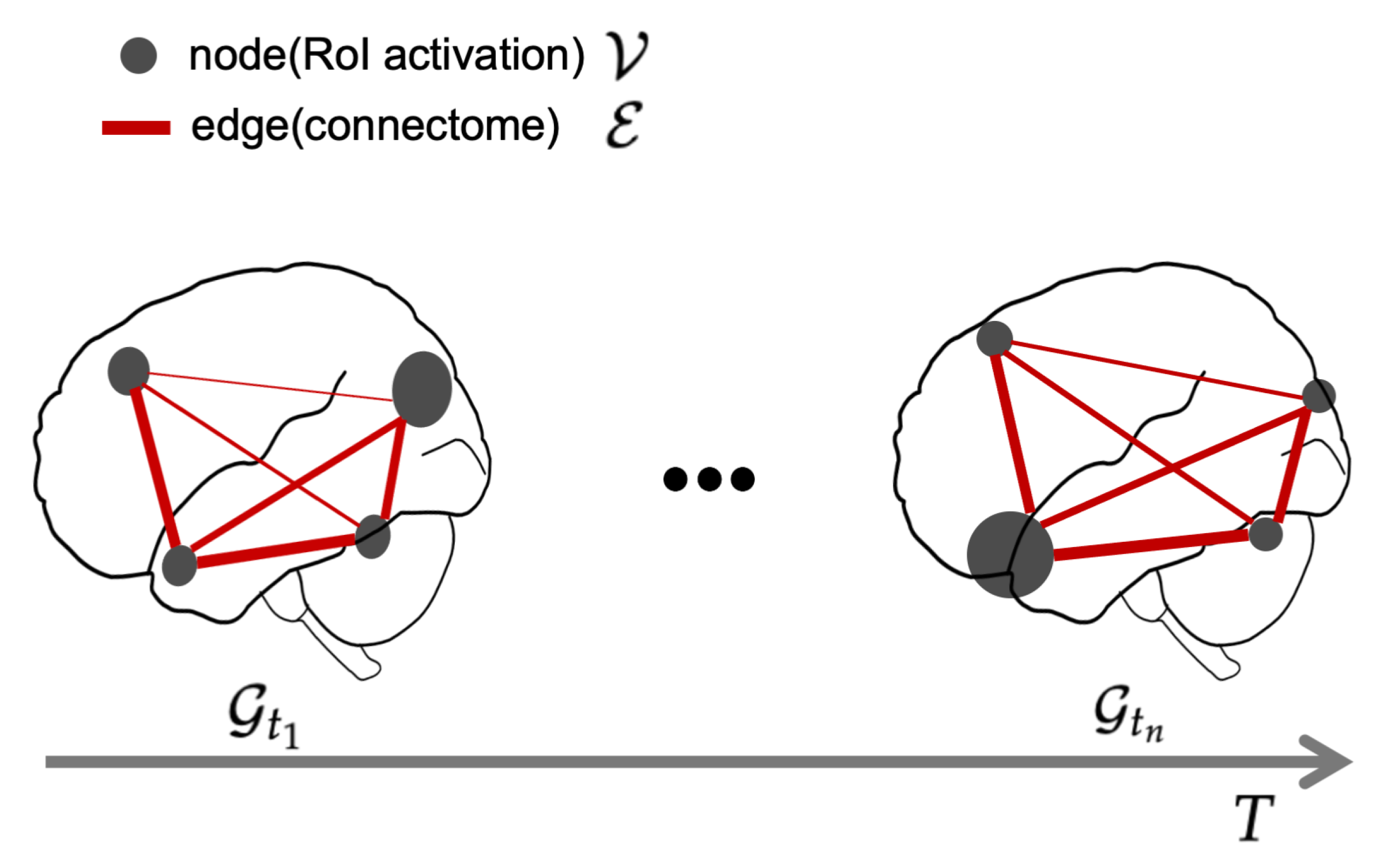
2.1. Time-Varying Brain Activity as a Graph

Before introducing the concept of smoothness harmonics, it is necessary to model time-varying brain activity in terms of a static graph. Let ${\mathcal{G}}_t=(\mathcal{V},\mathcal{E})$ be an undirected graph on time t, where $\mathcal{V}$ represents the set of time-varying nodes, which can be represented as an N-dimensional feature representation. A graph signal can be represented by a function $f:\mathcal{V}\to {\mathbb{R}}^n$ that assigns a scalar value to each node at time t. The nodes are interconnected by a set of edges $\mathcal{E}\subset \mathcal{V}\times \mathcal{V}$, which can also be characterized as an $N\times N$ feature representation, i.e., $\mathcal{E}\in {\mathbb{R}}^{N\times N}$.

In time-varying brain activity, the nodes $\mathcal{V}$ can be interpreted as the brain activation patterns in the region-of-interest (RoI), while the edges represent the connectome between RoIs (Figure 1). Thus, a graph signal f can be represented as an $[N,T]$ matrix to express the cortical dynamics over N RoIs throughout T time points. Importantly, we choose to utilize a static graph ($\mathcal{E}$) instead of a dynamic graph that assumes the graph structures evolve over time (${\mathcal{E}}_t$) to represent time-varying brain activity. This preference for a static graph over a dynamic one arises for two reasons: Firstly, the validity and reliability of estimating dynamic functional connectomes are still under question, and it remains uncertain whether these estimated time-varying graph structures truly reflect the underlying neurophysiological processes [15,16]. Secondly, from an application perspective, employing a static graph significantly reduces the computational cost compared to the heavy computational burden associated with dynamic graph analysis.

2.2. Smoothness Harmonic

The concept of smoothness harmonics is based on the eigendecomposition analysis of the graph Laplacian. Formally, considering the previously defined graph $\mathcal{G}$ with N nodes (RoIs) and $N\times N$ edges (connectomes), we can compute the symmetric graph Laplacian $\mathbf{L}\left(\mathcal{G}\right)$ using $\mathbf{L}\left(\mathcal{G}\right)=D-A$, where D is the degree matrix and A is the adjacency matrix. In an undirected graph, the adjacency matrix A can be represented as $\mathcal{E}$, where $A_{i,j}={\mathcal{E}}_{i,j}$. This adjacency matrix can be derived from the functional connectome [17]. The degree matrix D can be computed as $D={\sum }_{j=1}^{N}A(i,j)$.

According to graph theory [18,19], smoothness refers to the degree of variation exhibited by a graph signal f across the nodes of a graph $\mathcal{G}$. Conventionally, the smoothness of a graph can be quantified using the quadratic form of the graph Laplacian, $f^T\mathbf{L}\left(\mathcal{G}\right)f$. In the context of fMRI signals, which are predominantly characterized by ultra-slow oscillations, we propose measuring the smoothness of a graph based on the least-varying component, namely the first eigenvector associated with the smallest eigenvalue in the eigendecomposition of the graph Laplacian.

Let k denote the number of eigenvectors. We can obtain the eigenvector matrix ${\mathbf{U}}_k$ as follows: $\mathbf{L}\left(\mathcal{G}\right)={\mathbf{U}}_k\mathrm{\Lambda }{\mathbf{U}}_k^T$, where $\mathrm{\Lambda }$ is a diagonal matrix with the Laplacian eigenvalues ${\lambda }_1,{\lambda }_2,\dots ,{\lambda }_k$, and ${\mathbf{U}}_k$ is the orthonormal matrix consisting of the corresponding eigenvectors (arranged as columns).

Since the first eigenvector of the eigendecomposed graph Laplacian is associated with the low-frequency and slowly varying component of the graph [20], we extract the first eigenvector, denoted as ${\mathbf{U}}_{k=1}$, to represent the slowly varying harmonic of the graph [17]. These slowly varying harmonics in cortical dynamics are believed to reflect changes in the brain’s local network architecture, such as the reconfiguration of small-scale functional modules or alterations in the strength of local connections [21]. By utilizing the extracted slowly varying harmonic ${\mathbf{U}}_{k=1}$, we derive the resulting smoothness harmonics (${\mathbb{E}}_{\mathrm{temp}}\left(f\right)$), which quantify the extent to which a graph signal f varies on the slowly varying harmonic, as follows:

$${\mathbb{E}}_{\mathrm{temp}}\left(f\right)={(f\otimes {\mathbf{U}}_{k=1})}^T·f,$$

(1)

where ⊗ denotes the broadcastable element-wise multiplication, allowing the resulting matrix ${(f\otimes {\mathbf{U}}_{k=1})}^T$ to obtain the size of $[T,N]$.

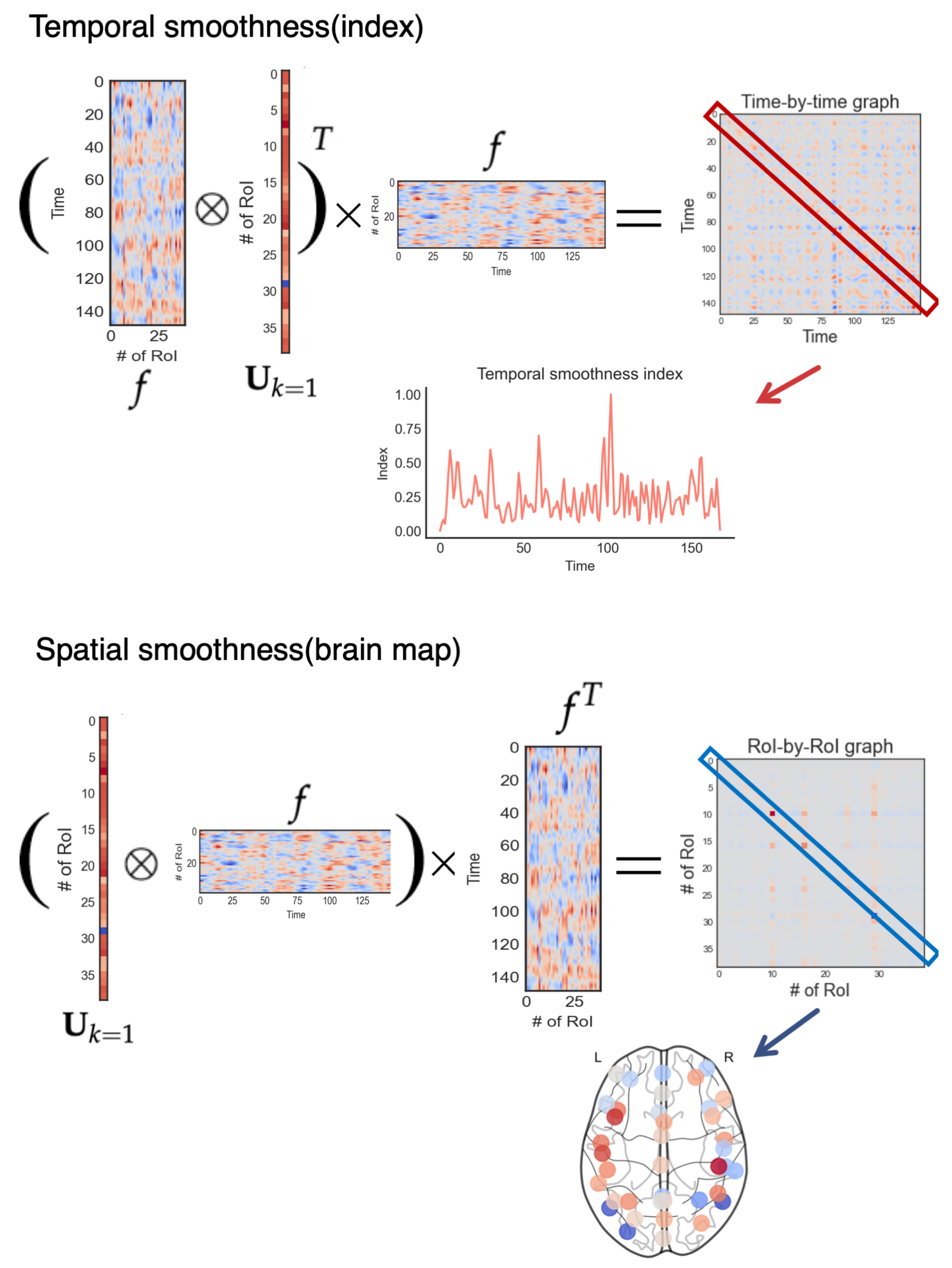
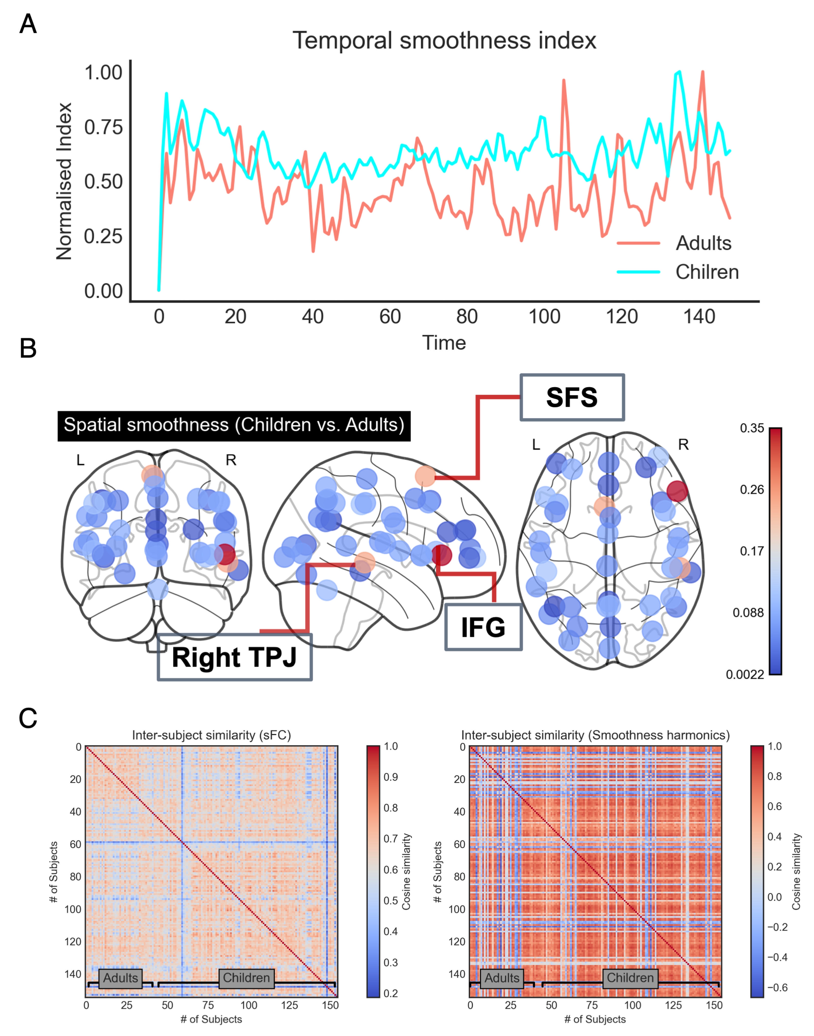
2.3. Temporal Smoothness Index and Spatial Smoothness Brain Map

The previously defined smoothness harmonic (${\mathbb{E}}_{\mathrm{temp}}$) captures the slowly varying harmonic in terms of the time-by-time graph, revealing how these harmonics propagate over time. To obtain a simplified measure of the temporal smoothness harmonic, we extract the diagonal component from the time-by-time graph. This yields a scalar indicator that conveniently represents the level of temporal smoothness harmonic (see Figure 2, upper plot).

Interestingly, since the graph signal f contains both spatial and temporal information regarding the recorded cortical dynamics, we can calculate a spatial version of the smoothness harmonic (${\mathbb{E}}_{\mathrm{spat}}\left(f\right)$) using the following procedure:

$${\mathbb{E}}_{\mathrm{spat}}\left(f\right)=({\mathbf{U}}_{k=1}\otimes f)·f^T.$$

(2)

where the broadcastable operator ⊗ ensures element-wise multiplication between ${\mathbf{U}}_{k=1}$ and f; we broadcast ${\mathbf{U}}_{k=1}$ to match the dimensions of f, resulting in a matrix $({\mathbf{U}}_{k=1}\otimes f)$ with a size of $[N,T]$.

The diagonal elements of spatial smoothness harmonics unveil the spatial distribution of smoothness harmonics across the cortex, represented as a region-of-interest (RoI)-by-RoI graph that illustrates their spatial propagation pattern. This graph can be projected onto a brain surface to generate (a) brain map(s) for visualization purposes (see Figure 2, lower plot). The full Python notebook showcasing the computational steps for producing ${\mathbb{E}}_{\mathrm{temp}}\left(f\right)$ and ${\mathbb{E}}_{\mathrm{spat}}\left(f\right)$ is available at https://github.com/LeonBai/SH (accessed on 1 April 2023).

3. Application in Age-Development fMRI Data

We provide a demonstration of the efficacy of our proposed smoothness harmonics in capturing age-related variations in cortical dynamics using fMRI data. Our spatiotemporal smoothness harmonics surpass conventional static functional connectivity patterns, offering a more comprehensive understanding of cortical dynamics in children and adults that reflects their developmental changes in cognition.

3.1. Dataset and Preprocessing

The fMRI data utilized in this study were sourced from the age-development (children versus adults) movie-watching dataset released by [14]. The selection of this passive stimulus fMRI dataset, as opposed to task-evoked or resting-state fMRI datasets, was driven by two primary considerations. Firstly, passive stimulus perception has been observed to significantly reduce head motion, resulting in enhanced imaging quality compared to task-evoked fMRI setups [22]. Secondly, given that all subjects viewed the same movie clip, we assumed near-identical stimulus perception across all subjects, facilitating group-wise analysis without necessitating intricate between-subject alignment techniques typically employed in resting-state fMRI datasets [23].

In the age-development study, a total of 155 subjects participated, comprising 33 adults and 122 children. During the MRI acquisition session, all subjects were instructed to watch a silent 5.6-min animated movie titled “Partly Cloudy” [24]. Structural and functional MRI data were acquired using a three-Tesla scanner equipped with a standard 32-channel head coil. The anatomical images of each subject were subsequently normalized to the Montreal Neurological Institute (MNI) template. Following the removal of motion-correlated artifacts, each subject’s neuroimaging time course consisted of 149 time intervals with a repetition time (TR) of 2 s. To facilitate preprocessing, skull stripping was performed using the individual T1-weighted (T1w) reference image, followed by spatial normalization to the widely used nonlinear MNI152 template, specifically, the MNI152nlin2009ascym template (the default spatial template used in the fMRI-prep application for fMRI image preprocessing: https://fmriprep.org/en/stable/spaces.html (accessed on 1 May 2022)).

3.2. f and Estimated $\mathcal{E}$

To extract region-of-interest (RoI) signals from the voxel-wise fMRI data, we utilized the MSDL brain atlas [25], which provides an intermediate parcellation scheme consisting of 39 nodes. This atlas allowed us to define distinct brain regions of interest. By mapping the fMRI data onto this parcellation, we obtained subject-level graph signal matrices (f) for all 155 participants. Each matrix had a size of $[39,149]$, where the first dimension represented the spatial resolution (39 RoIs) and the second dimension represented the temporal resolution (149 time intervals).

To estimate the functional connectome, we computed the Pearson’s correlation coefficient between each pair of time series ${\mathcal{V}}_t$ for the 155 subjects. This resulted in 155 subject-level connectivity matrices ($\mathcal{E}$) with dimensions of $[39,39]$, where each element represents the correlation strength between two corresponding brain regions (nodes) in the MSDL brain atlas. These estimated connectivity matrices can be interpreted as static functional connectomes (sFCs) and serve as a representation of the functional connectivity patterns for each subject. These sFCs are used for comparative analyses in our study, allowing us to evaluate the performance of the proposed smoothness harmonics against conventional static functional connectivity measures.

3.3. Extracted Smoothness Harmonics and Their Merits

The analysis of the smoothness harmonics, both in terms of spatial smoothness brain maps (${\mathbb{E}}_{\mathrm{spat}}\left(f\right)$) and temporal smoothness index (${\mathbb{E}}_{\mathrm{temp}}\left(f\right)$), reveals distinct cortical dynamics between children and adults. Figure 3A illustrates the results, showing that children exhibit overall more stable brain activity throughout the movie clip compared to adults. This finding aligns with previous research suggesting that children may demonstrate greater attentiveness during cartoon-watching situations compared to adults [14].

Of particular interest is the significant difference observed in the spatial smoothness of brain maps between adults and children (Figure 3B). In cortical regions associated with higher cognitive functions and the development of the theory of mind (caring about others’ thoughts), such as the superior frontal sulcus (SFS), right temporoparietal junction (Right TPJ) [26], and the inferior frontal gyrus (IFG) [27], notable distinctions between children and adults are observed. These findings are consistent with previous studies investigating the neural basis of developmental differences between children and adults in developing the theory of mind [28,29,30].

The use of smoothness harmonics as discriminative features in inter-subject similarity and between-group classification analyses yielded interesting results. Figure 3C and the first row of

Table 1. Usages of sFCs and smoothness harmonics in inter-subject similarity and between-group analyses.

	sFCs	Smoothness Harmonics
Inter-subject similarity	Overall: $0.628$	Overall: $0.446$
	Between-adults: $0.318$	Between-adults: $0.654$
	Between-children: $0.624$	Between-children: $0.632$
Between-group classification accuracy (%)	$64.6\pm 2.12$	$80.7\pm 1.13$

demonstrate that highly consistent inter-subject brain patterns were identified when using smoothness harmonics for both adults and children. In contrast, the utilization of the static functional connectomes (sFCs) as an alternative only achieved compatible inter-subject similarity for the children’s group, as indicated by the overall score of 0.628.

It is noteworthy that the overall score for smoothness harmonics was much lower (0.446) compared to that of the sFC approach. This lower score can be interpreted as a failure of the sFC approach to effectively capture the group-wise differences between adults and children. These results highlight the superior performance of smoothness harmonics as discriminative features in capturing meaningful variations and distinctions in cortical dynamics between different age groups.

Notably, in our attempt to classify phenotypes between children and adults using both sFC and extracted smoothness as discriminative features, we conducted a simple classification analysis. Since the classification accuracy is largely determined by the classifier and the volume of the discriminating features used in training [31], we employed the respective features (sFC: $39\times 39$; smoothness harmonics: $39\times 39$) to train an individual SVM and evaluated its classification performance on the testing dataset (training/testing ratio: 2/8). Over 10 repetitions (the second row of Table 1), the smoothness harmonics demonstrated a clear empirical advantage over sFC in classifying adults from children.

Additionally, we also applied an off-the-shelf graph embedding approach, namely the Graph2Vec method [12], to the age-development dataset, producing an identical number of discriminative features ($39\times 39$) for training another independent SVM. When evaluated on the same testing set, these graph-embedding features yielded an average classification accuracy of $76.6\%$, demonstrating the superiority of our approach over other static graph analysis methods.

These results provide compelling evidence that the smoothness harmonics capture meaningful differences in cortical dynamics between children and adults, highlighting the potential of this approach for studying developmental processes and cognitive functions.

4. Discussion

In this communication, we present graph-based smoothness harmonics as a powerful tool for capturing the slowly varying spatiotemporal patterns of cortical dynamics in fMRI data. The temporal smoothness index and spatial smoothness brain map derived from the smoothness harmonics provide valuable insights into the propagation of slowly varying cortical dynamics across the entire cortex over time. By applying this approach to age-development fMRI data, we demonstrated the versatility of smoothness harmonics in discerning differences in cortical dynamics between adults and children, thereby reflecting the age-related variations in the development of the theory of mind. These findings highlight the potential of smoothness harmonics as a valuable tool for investigating and understanding cortical dynamics in various contexts.

Undoubtedly, graph analysis has been widely employed in the study of cortical dynamics, ranging from early attempts to model brain connectomes as small-world networks [6,32] to more recent advancements in deep graph neural networks for learning nodal representations of graph signals [12,33] and exploring complex brain topology to investigate neuropsychiatric disorders [34]. However, our proposed smoothness harmonic approach stands out from these existing methods in two key aspects. Firstly, our method is specifically designed for the analysis of fMRI data. It captures the predominant slow-frequency oscillations that are characteristic of fMRI signals through the extraction of smoothness harmonics. This targeted approach enables a more-focused examination of cortical dynamics in the context of fMRI studies. Secondly, unlike the complex learning algorithms used in other approaches, our smoothness harmonic approach relies solely on the well-established eigendecomposition framework. This ensures a straightforward and easily implementable methodology. This simplicity and convenience make our approach accessible to researchers and facilitates its application in diverse fMRI studies.

The introduction of smoothness harmonics opens up exciting future opportunities to explore and compare various types of neuropsychiatric disorders based on their extracted smoothness harmonics. Additionally, as a potential avenue for future research, the concept of smoothness harmonics can be applied to dynamic graph analysis to address the growing demand for dynamic functional connectivity analysis [35]. However, when applying this concept to other neuroimaging modalities such as EEG and MEG data, it is important to consider incorporating additional non-slow harmonics to accommodate the specific characteristics of those modalities. Overall, the graph-based smoothness harmonic has the potential to provide valuable insights into the spatiotemporal dynamics of brain activity and contribute to advancements in the field of neuroscience.

References

1. Friston, K.J.; Kahan, J.; Razi, A.; Stephan, K.E.; Sporns, O. On nodes and modes in resting state fMRI. Neuroimage 2014, 99, 533–547. [Google Scholar] [CrossRef] [PubMed] [Green Version]
2. Logothetis, N.K. What we can do and what we cannot do with fMRI. Nature 2008, 453, 869–878. [Google Scholar] [CrossRef] [PubMed]
3. Friston, K.J.; Holmes, A.P.; Poline, J.; Grasby, P.; Williams, S.; Frackowiak, R.S.; Turner, R. Analysis of fMRI time-series revisited. Neuroimage 1995, 2, 45–53. [Google Scholar] [CrossRef]
4. Borogovac, A.; Asllani, I. Arterial spin labeling (ASL) fMRI: Advantages, theoretical constrains and experimental challenges in neurosciences. Int. J. Biomed. Imaging 2012, 2012, 818456. [Google Scholar]
5. Niazy, R.K.; Xie, J.; Miller, K.; Beckmann, C.F.; Smith, S.M. Spectral characteristics of resting state networks. In Progress in Brain Research; Elsevier: Amsterdam, The Netherlands, 2011; Volume 13, pp. 259–276. [Google Scholar]
6. Bullmore, E.; Sporns, O. Complex brain networks: Graph theoretical analysis of structural and functional systems. Nat. Rev. Neurosci. 2009, 10, 186–198. [Google Scholar] [CrossRef] [PubMed]
7. Mears, D.; Pollard, H.B. Network science and the human brain: Using graph theory to understand the brain and one of its hubs, the amygdala, in health and disease. J. Neurosci. Res. 2016, 94, 590–605. [Google Scholar] [CrossRef]
8. Telesford, Q.K.; Simpson, S.L.; Burdette, J.H.; Hayasaka, S.; Laurienti, P.J. The brain as a complex system: Using network science as a tool for understanding the brain. Brain Connect. 2011, 1, 295–308. [Google Scholar] [CrossRef] [Green Version]
9. Farahani, F.V.; Karwowski, W.; Lighthall, N.R. Application of graph theory for identifying connectivity patterns in human brain networks: A systematic review. Front. Neurosci. 2019, 13, 585. [Google Scholar] [CrossRef]
10. Grohe, M. word2vec, node2vec, graph2vec, x2vec: Towards a theory of vector embeddings of structured data. In Proceedings of the 39th ACM SIGMOD-SIGACT-SIGAI Symposium on Principles of Database Systems, Portland, OR, USA, 14–19 June 2020; pp. 1–16. [Google Scholar]
11. Levakov, G.; Faskowitz, J.; Avidan, G.; Sporns, O. Mapping individual differences across brain network structure to function and behavior with connectome embedding. Neuroimage 2021, 242, 118469. [Google Scholar] [CrossRef]
12. Narayanan, A.; Chandramohan, M.; Venkatesan, R.; Chen, L.; Liu, Y.; Jaiswal, S. graph2vec: Learning distributed representations of graphs. arXiv 2017, arXiv:1707.05005. [Google Scholar]
13. Levy, B. Laplace-beltrami eigenfunctions towards an algorithm that “understands” geometry. In Proceedings of the IEEE International Conference on Shape Modeling and Applications 2006 (SMI’06), Matsushima, Japan, 14 June 2006; p. 13. [Google Scholar]
14. Richardson, H.; Lisandrelli, G.; Riobueno-Naylor, A.; Saxe, R. Development of the social brain from age three to twelve years. Nat. Commun. 2018, 9, 1–12. [Google Scholar] [CrossRef] [PubMed] [Green Version]
15. Preti, M.G.; Bolton, T.A.; Van De Ville, D. The dynamic functional connectome: State-of-the-art and perspectives. Neuroimage 2017, 160, 41–54. [Google Scholar] [CrossRef] [PubMed]
16. Leonardi, N.; Van De Ville, D. On spurious and real fluctuations of dynamic functional connectivity during rest. Neuroimage 2015, 104, 430–436. [Google Scholar] [CrossRef] [Green Version]
17. Atasoy, S.; Donnelly, I.; Pearson, J. Human brain networks function in connectome-specific harmonic waves. Nat. Commun. 2016, 7, 10340. [Google Scholar] [CrossRef] [PubMed] [Green Version]
18. Dong, X.; Thanou, D.; Frossard, P.; Vandergheynst, P. Learning Laplacian matrix in smooth graph signal representations. IEEE Trans. Signal Process. 2016, 64, 6160–6173. [Google Scholar] [CrossRef] [Green Version]
19. Stankovic, L.; Mandic, D.; Dakovic, M.; Brajovic, M.; Scalzo, B.; Constantinides, T. Graph Signal Processing—Part I: Graphs, Graph Spectra, and Spectral Clustering. arXiv 2019, arXiv:1907.03467. [Google Scholar]
20. Belkin, M.; Niyogi, P. Laplacian eigenmaps for dimensionality reduction and data representation. Neural Comput. 2003, 15, 1373–1396. [Google Scholar] [CrossRef] [Green Version]
21. Buzsaki, G.; Draguhn, A. Neuronal oscillations in cortical networks. Science 2004, 304, 1926–1929. [Google Scholar] [CrossRef] [Green Version]
22. Vanderwal, T.; Kelly, C.; Eilbott, J.; Mayes, L.C.; Castellanos, F.X. Inscapes: A movie paradigm to improve compliance in functional magnetic resonance imaging. Neuroimage 2015, 122, 222–232. [Google Scholar] [CrossRef] [Green Version]
23. Haxby, J.V.; Guntupalli, J.S.; Connolly, A.C.; Halchenko, Y.O.; Conroy, B.R.; Gobbini, M.I.; Hanke, M.; Ramadge, P.J. A common, high-dimensional model of the representational space in human ventral temporal cortex. Neuron 2011, 72, 404–416. [Google Scholar] [CrossRef] [Green Version]
24. Reher, K.; Sohn, P. Partly Cloudy [Motion Picture]; Pixar Animation Studios and Walt Disney Pictures: Burbank, CA, USA, 2009. [Google Scholar]
25. Varoquaux, G.; Gramfort, A.; Pedregosa, F.; Michel, V.; Thirion, B. Multi-subject dictionary learning to segment an atlas of brain spontaneous activity. In Proceedings of the Biennial International Conference on Information Processing in Medical Imaging, Irsee, Germany, 3 July 2011; pp. 562–573. [Google Scholar]
26. Saxe, R.; Kanwisher, N. People thinking about thinking people: The role of the temporo-parietal junction in “theory of mind”. Neuroimage 2003, 19, 1835–1842. [Google Scholar] [CrossRef]
27. Gallagher, H.L.; Frith, C.D. Functional imaging of ’theory of mind’. Trends Cogn. Sci. 2003, 7, 77–83. [Google Scholar] [CrossRef] [PubMed] [Green Version]
28. Kobayashi, C.; Glover, G.H.; Temple, E. Children’s and adult’s neural bases of verbal and nonverbal theory of mind. Neuropsychologia 2007, 45, 1522–1532. [Google Scholar] [CrossRef] [PubMed] [Green Version]
29. Gallagher, H.L.; Happé, F.; Brunswick, N.; Fletcher, P.C.; Frith, U.; Frith, C.D. Reading the mind in cartoons and stories: An fMRI study of ‘theory of mind’in verbal and nonverbal tasks. Neuropsychologia 2000, 38, 11–21. [Google Scholar] [CrossRef]
30. Gweon, H.; Dodell-Feder, D.; Bedny, M.; Saxe, R. Theory of mind performance in children correlates with functional specialization of a brain region for thinking about thoughts. Child Dev. 2012, 83, 1853–1868. [Google Scholar] [CrossRef]
31. Kwon, O.; Sim, J.M. Effects of data set features on the performances of classification algorithms. Expert Syst. Appl. 2013, 40, 1847–1857. [Google Scholar] [CrossRef]
32. Rubinov, M.; Sporns, O. Complex network measures of brain connectivity: Uses and interpretations. Neuroimage 2010, 52, 1059–1069. [Google Scholar] [CrossRef]
33. Yousefian, A.; Shayegh, F.; Maleki, Z. Detection of autism spectrum disorder using graph representation learning algorithms and deep neural network, based on fMRI signals. Front. Syst. Neurosci. 2022, 16, 904770. [Google Scholar] [CrossRef]
34. Suo, X.; Lei, D.; Li, K.; Chen, F.; Li, F.; Li, L.; Huang, X.; Lui, S.; Li, L.; Kemp, G.J.; et al. Disrupted brain network topology in pediatric posttraumatic stress disorder: A resting-state fMRI study. Hum. Brain Mapp. 2015, 36, 3677–3686. [Google Scholar] [CrossRef]
35. Lurie, D.J.; Kessler, D.; Bassett, D.S.; Betzel, R.F.; Breakspear, M.; Kheilholz, S.; Kucyi, A.; Liégeois, R.; Lindquist, M.A.; McIntosh, A.R.; et al. Questions and controversies in the study of time-varying functional connectivity in resting fMRI. Netw. Neurosci. 2020, 4, 30–69. [Google Scholar] [CrossRef]
Figure 1. Time-varying brain activity as a graph. The sizes and widths of nodes and edges represent the strength of their respective feature values. We characterize the brain activity that evolves through T time points (representing the duration of recorded brain activity) as a graph. In this graph, the nodal features represent the region-of-interest (RoI) brain activations V , while the edges represent the connectomes E between RoIs. As time progresses, i.e., from G t 1 to G t n , the nodal features change accordingly, while the edge features remain the same.
Applsci 13 07130 g001
Figure 2. Temporal and spatial smoothness harmonics to reflect the spatiotemporal pattern of cortical dynamics. Upper plot: the production process of temporal smoothness index. The temporal smoothness index of a graph can be obtained from the diagonal elements of a time-by-time graph, which illustrates how slowly varying cortical dynamics evolve over time. Lower plot: the production process of the spatial smoothness brain map. The spatial smoothness brain map is obtained by projecting a region-of-interest (RoI)-by-RoI graph onto a brain surface map. The diagonal elements of this graph indicate how slowly varying cortical dynamics propagate across the cortex.
Applsci 13 07130 g002
Figure 3. Extracted smoothness harmonics in the age-development fMRI dataset [14]. (A) Attained temporal smoothness indexes for the group-wise adult and child fMRI data. The raw indexes were normalized to the range of [ 0 , 1 ] for ease of comparison. (B) Differences in the extracted spatial smoothness harmonics between adults and children are represented in a pairwise spatial format, with the color bar indicating the harmonic value difference between the two groups. The three most-differentiated brain regions, highlighted in light red colors, are the superior frontal sulcus (SFS), the right temporoparietal junction (Right TPJ), and the inferior frontal gyrus (IFG). The produced brain maps are displayed for the hemispheres from coronal, sagittal, and horizontal views from left to right. (C) The inter-subject similarity was assessed based on either the static functional connectome (sFC) on the left or the estimated smoothness patterns on the right. In both correlation matrices, the first 33 subjects represent adults, while the remaining subjects represent children. The color bar indicates the cosine similarity. The abbreviation index indicates that sFC stands for static functional connectome.
Applsci 13 07130 g003