GRU Neural Network Based on CEEMDAN–Wavelet for Stock Price Prediction

Abstract

Stock indices are considered to be an important indicator of financial market volatility in various countries. Therefore, the stock market forecast is one of the challenging issues to decrease the uncertainty of the future direction of financial markets. In recent years, many scholars attempted to use different conventional statistical and deep learning methods to predict stock indices. However, the non-linear financial noise data will usually cause stochastic deterioration and time lag in forecast results, resulting in existing neural networks that do not demonstrate good prediction results. For this reason, we propose a novel framework to combine the gated recurrent unit (GRU) neural network with the complete ensemble empirical mode decomposition of adaptive noise (CEEMDAN) to predict the stock indices with better accuracy, in which the wavelet threshold method is especially used to denoise high-frequency noises in the sub-signals to exclude noise interference for future data predictions. Firstly, we choose representative datasets collected from the closing prices of S&P500 and CSI 300 stock indices to evaluate the proposed GRU-CEEMDAN–wavelet model. Additionally, we compare the improved model to the traditional ARIMA and several modified neural network models using different gate structures. The result shows that the mean values of MSE and MAE for GRU based on CEEMDAN–wavelet are the smallest by significance analysis. Overall, we found that our model could improve prediction accuracy and alleviates the time lag problem.

1. Introduction

With the rapid development of internet finance and big data technology, fundamental and technical analysis forecasting schemes are no longer popular today, because the stock market is highly random and volatile. The price of the financial market especially has been influenced by various factors, and the ambiguity of stock data makes the learning-based process more difficult [1]. To meet investors’ needs, a greater emphasis on data forecasting in recent years has led to many advances in the neural network [2].

Deep learning originated from artificial neural networks (ANNs), whose basic framework is to build a multi-layer structure and extract features from the input data for combination to obtain a more abstract data structure. Ivakhnenko et al. developed the first working neural network, which was demonstrated in the computer identification system [3]. However, the information learning process did not use a backpropagation algorithm for training the network in this model. Later, Rumelhart et al. proposed the error backpropagation algorithm [4], now known as the BP neural network, which collected the errors generated by the system during the cycle and returns them to the outputs. After that, they applied these errors to adjust the weights of every single neuron, resulting in an artificial neural network. The appearance of BP solved the problem of GMDH, which cannot carry out the backpropagation. Currently, the BP neural network model has penetrated into many cutting-edge fields such as pattern recognition [5], speech processing [6], image processing, nonlinear optical [7], financial data forecasting, etc. Huang et al. used the BP neural network for regional logistics demand forecasting (RLDF) [8], but BP neural networks have very obvious and fatal drawbacks—low learning efficiency, slow convergence, and a tendency to fall into local minima.

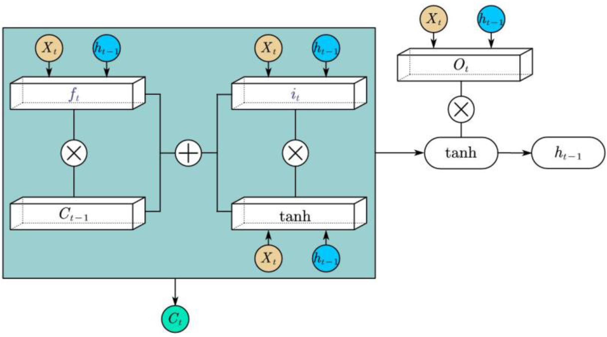
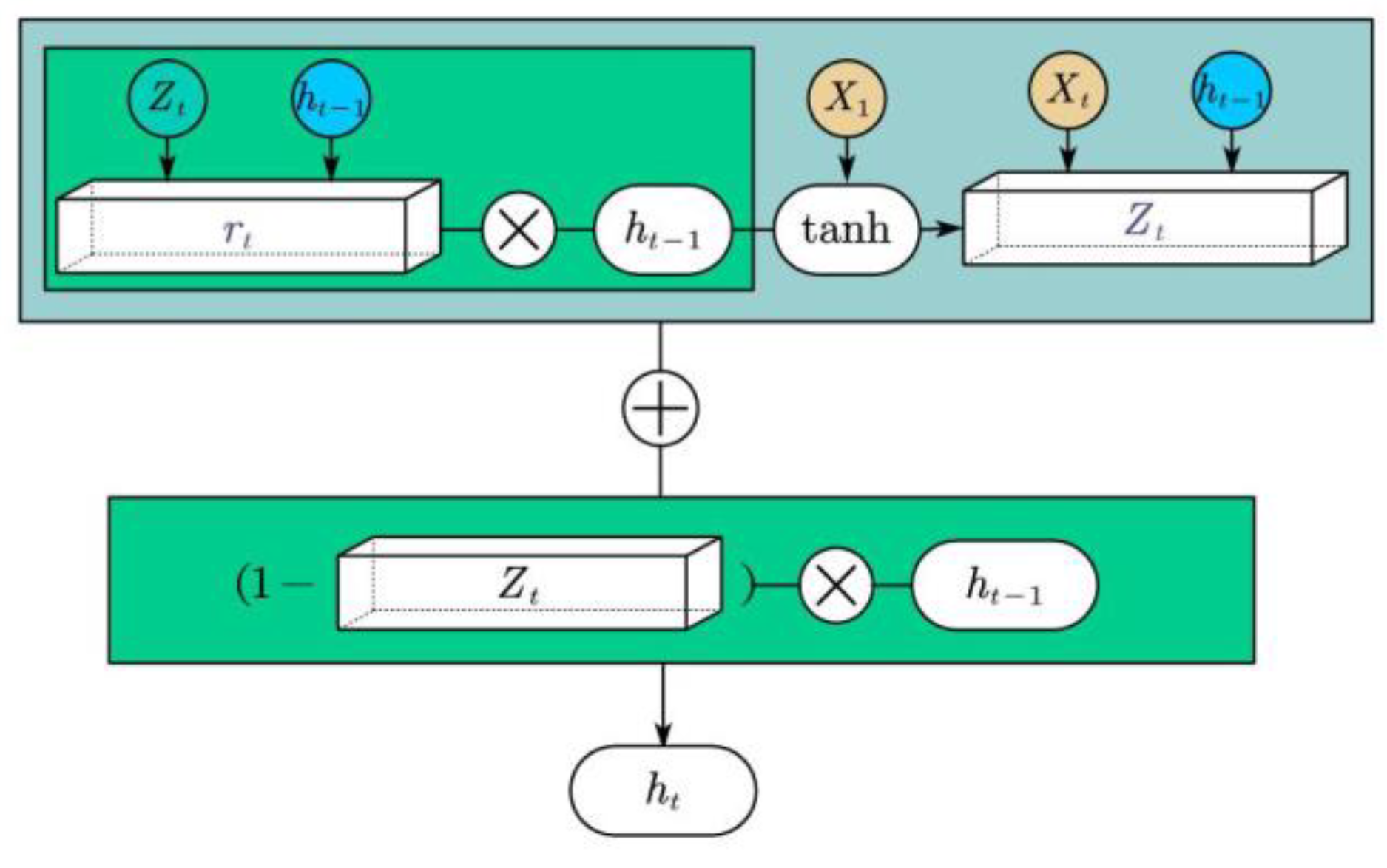
Schmidhuber et al. [9] elucidated a new recurrent neural network architecture named long short-term memory. This special neural recurrent network could deal with the problem of gradient diffusion and explosion so that it can be used for data modeling of long time series. In 2017, Selvin et al. [10] compared traditional GARCH models with LSTM to illustrate that LSTM outperforms other previous algorithms. LSTM is a special RNN structure; it is suitable for learning, classifying, processing, and predicting time series from experience, it consists of three gate structures, and each of them can filter the useless information more efficiently to decide which information needs to be used next time or which information needs to be discarded. Both LSTM and gate recurrent unit [11] (GRU) are variants of RNN, but compared with LSTM, GRU has one less gate structure, fewer parameters, and faster convergence and iteration speed.

However, these neural networks do not take into account the noise of data when making predictions. The initial signal contains noise that is unfavorable to the forecast. To improve the accuracy by continuously optimizing the prediction models, the preprocessing methods of data input are also improved during a series of research. For example, Büyükahin et al. [12] proved that mode decomposition techniques can reduce signal noise pollution and improve the accuracy of prediction.

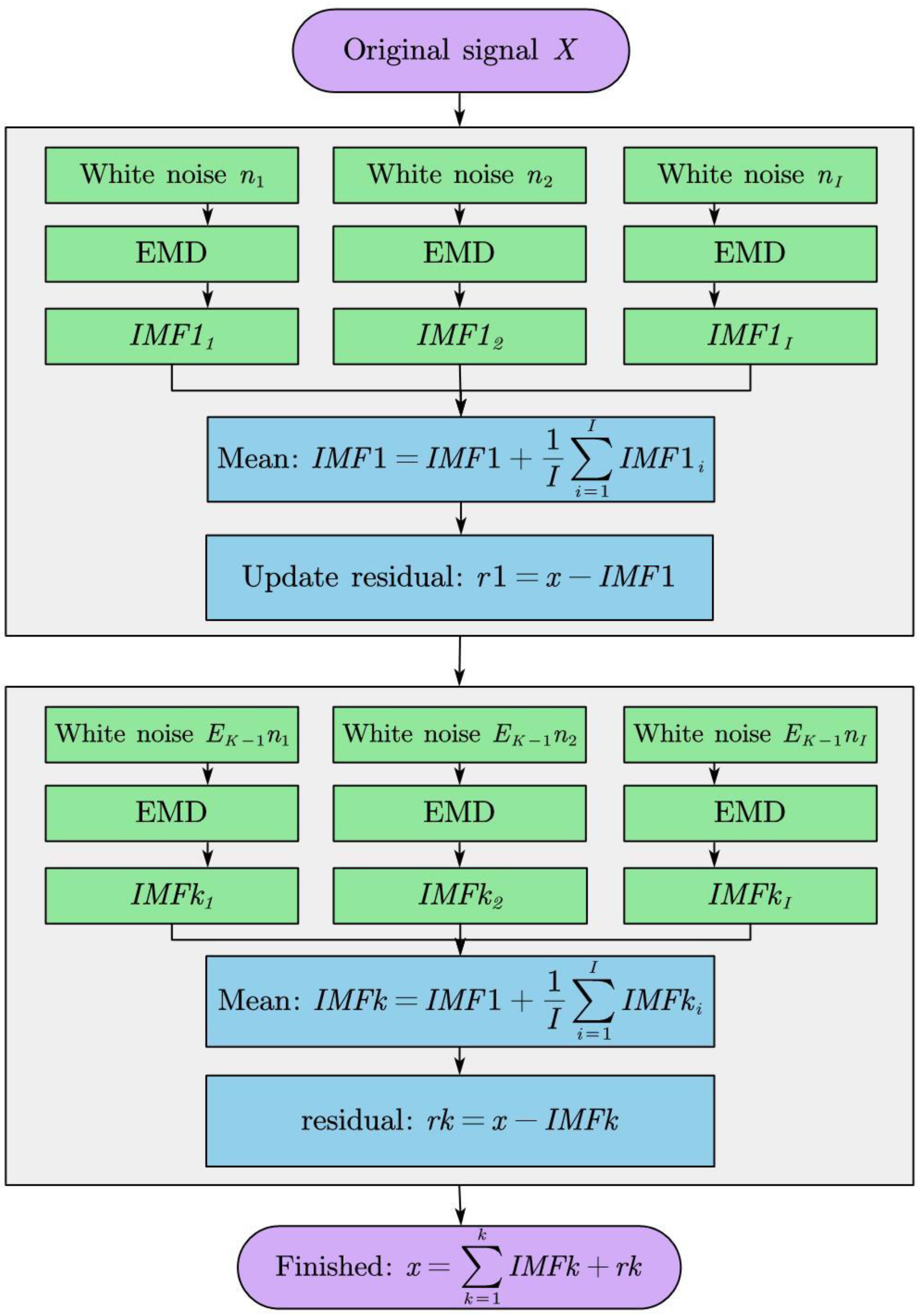
Empirical mode decomposition (EMD) was discovered by Huang et al. [13] and taken as a new type of adaptive signal time–frequency processing method without requiring any basis functions, which is so different from harmonic function and wavelet basis functions. Theoretically, EMD can be applied to any type of signal decomposition in any field, such as [14] used to decompose sonar signals in the ocean, and in the medical field, it is used to extract features from electroencephalogram (EEG) signals [15].

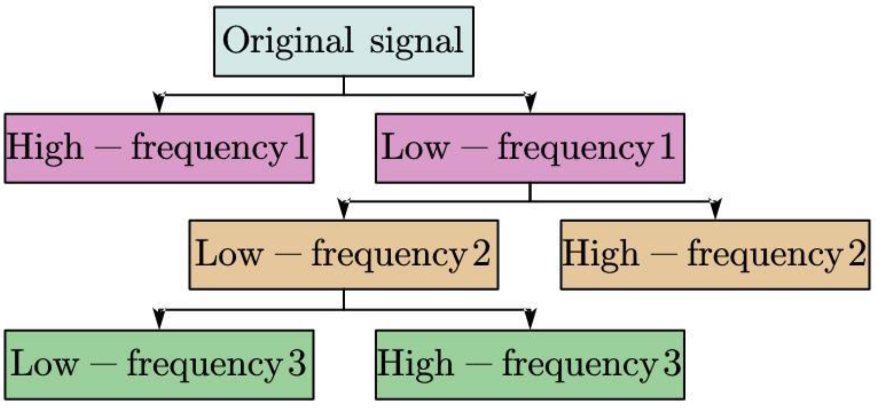
Before EMD, there existed another method called wavelet transform. The concept of wavelet transform was introduced by Morlet, but, unfortunately, this method was not recognized by mathematicians at that time until Meyer accidentally constructed a real wavelet basis and collaborated with Mallat to establish the multi-resolution analysis (MRA) [16]; since then, wavelet analysis has been generally accepted and flourished.

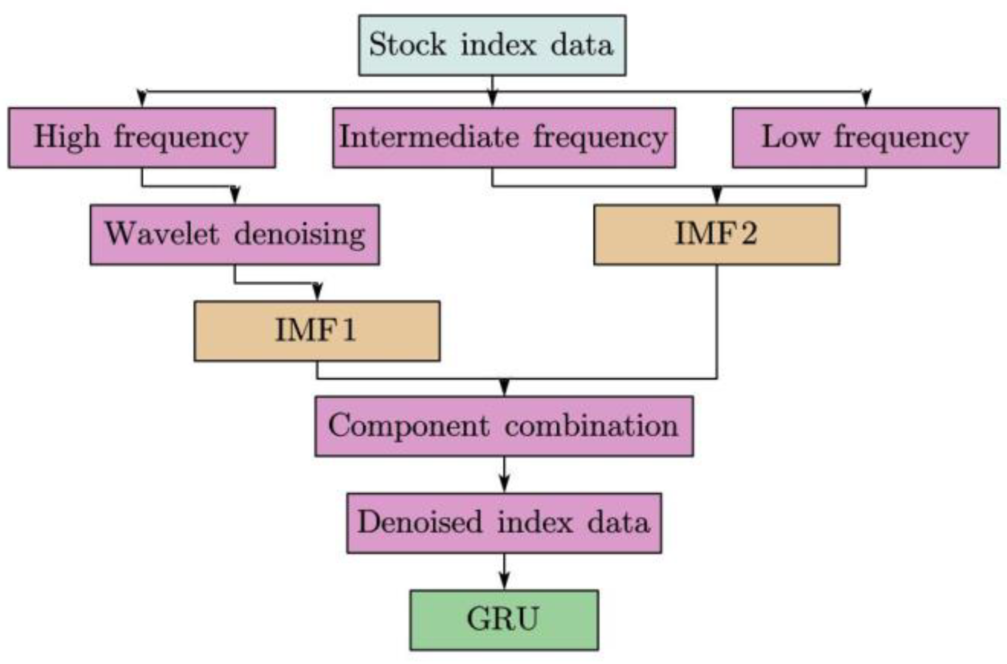
However, the applications of certain single models always have poor forecasting results, such as the ARIMA model, which utilizes only one set of data as input variables. To overcome the limitations of the traditional models, we combine a hybrid model using multi-dimensional variables as input to forecast future data. Firstly, CEEMDAN [17] is used to decompose the original signal, and then the high-frequency signal is especially denoised by using the wavelet transform function. Finally, the reintegrated signal is put into the GRU neural network for assessment and forecast. The result shows that our framework model has better performance than the extant models.

Compared with traditional methods, deep models have been widely used to predict time series with the following advantages: data-driven, adaptive, as well as a higher ability to analyze inaccurate and noisy data. Deep models can be trained with large amounts of nonlinear data, capturing more abstract nonlinear relationships between data; thus, it was used to solve nonlinear problems more satisfactorily than traditional machine learning algorithms. In recent work of deep models on the field of stock price prediction, Swathi et al. [18] present a new novel teaching and learning-based optimization (TLBO) model with long short-term memory (LSTM)-based sentiment analysis for stock price prediction using Twitter data. The proposed method produced a greater accuracy. Zhao et al. [19] proposed a novel hybrid model SA-DLSTM to predict the stock market and simulation trading by combining an emotion-enhanced convolutional neural network, the denoising autoencoder, and LSTM models. SA-DLSTM has a good performance both in return and risk. It can help investors make wise decisions.

As mentioned above, neural computing methods are used in various fields, including data mining, stock prediction, image feature extraction, and so on. However, many scholars use only single historical data for forecasting, resulting in the intrinsic structure and variability of the stock market not being fully considered. Meanwhile, the inappropriate denoising process has caused a part of information loss. Hence, in this paper, we propose a new network architecture based on GRU and CEEMDAN to predict market direction, which collects multidimensional variables and decomposes high-frequency components using the wavelet function to improve prediction accuracy while maximizing information integrity.

This paper is organized as follows. Section 2 introduces the preliminary work of neural network prediction. Section 3 describes the design of the GRU neural network based on the CEEMDAN–wavelet. Section 4 presents the experiment setup and test process, and the results are obtained by comparative experiments. Section 5 shows the discussion in detail. In Section 6, the conclusion and future work directions are given.

2. Preliminaries

2.1. Related Work

A financial time series is a special type of time series that has a strong correlation before and after the data.

Before neural networks came out, many scholars used a simple autoregression integrated moving average model (ARIMA) to predict data trends [20]. Gradually, with the explosion of data volume, the limitations of the traditional model pose some new problems. In [21], they compared ARIMA and neural networks. The results showed that the neural networks outperformed the ARIMA model in predicting data from the New York Stock Exchange.

Therefore, many scholars use existing neural network models to forecast the stock market. In [22], they contradict the idea that the available information that affects current stock prices is composed of the market, and thus predicting future returns is not possible. Meanwhile, an information acquisition technique for data mining is proposed and used to make sure of the interrelationships of economic variables. In 2020, Lu et al. [23] first proposed a CNN-BiLSTM-AM approach for stock price prediction; they then added AM to capture the influence of feature states on the stock closing price. In 2020, Xiao et al. [24] used ARI-MA-LS-SVM to forecast. It can be concluded that the combined model based on ARI-MA-LS-SVM is more suitable for stock price forecasting than the single forecasting model, and the actual performance is better. Wang et al. [25] created a kind of new framework for forecasting the stock price named wavelet denoising-based backpropagation neural network (WDBP), and it also showed a great result.

At the same time, neural networks are also used in a variety of other areas. To optimize portfolios and asset allocation, Lee [26] proposed a novel framework that used wavelet transformation to decompose noise, and LSTM to reinforce learning; the result showed that the proposed HW LSTM RL structure outperformed other similar structures. In [27], they made some modifications to the original RNN and illustrate that they can further promote the accuracy of the original recurrent neural network language model (RNN-LM) by reducing computational complexity. Wang et al. [28] propose a novel deep neural network fusion embedding-based deep neural network (FEBDNN) to forecast retweeting behavior. All kinds of neural networks have grown by leaps and bounds in recent years, such as stacked or bidirectional structures. Stacked LSTM is considered to have better performance in accuracy and coverage speed than others after comparing the rest of the three variants (bidirectional LSTM, stacked GRU, and bidirectional GRU) in long and short-term stock markets [29]. In [30], they proposed a CBIR algorithm based on a convolutional neural network and bidirectional LSTM to detect vicious webpages information; the result showed that BCIR has improved the accuracy of malicious webpages detection more so than other ways.

Different sorts of signal decomposition connected with the neural network have also been proposed. For example, Hasan [31] used a hybrid EEMDAN-ANN model to predict COVID-19, and since the number of infected cases shows non-stationary and non-linear, they used EEMD to decompose the original signal and the artificial neural network (ANN) is then built on the signal that has completed denoising. The result illustrated that the proposed model provides a very valuable evaluation for predicting epidemic spread. Since the outbreak of COVID-19, it has spread faster than we could have imagined. A combination of artificial intelligence networks and particle swarm optimization was proposed by Jamous et al. [32], and they used a new method called PSOCoG to minimize processing time to maximize the accuracy of prediction. The result shows that ANN-PSOCoG outperformed other kinds of ANN models. Wu et al. [33] came up with an innovative deep coupling neural network (DCNN), which consists of a dataset-across network (DA-Net) and candidate-decision network (CD-Net), and the result shows that model robustness can be significantly improved by leveraging rich variations within and between different datasets. In the field of medicine, Kamnitsas et al. [34] presented a dual pathway, an 11-layer deep 3D convolutional neural network for the challenging task of brain lesion segmentation, and they analyze the development of a deeper and more discriminative 3D CNN. Their work has been recognized in many disease areas. Cascading MARS with DL is a novel attempt in [35]. The importance of reducing computational complexity is emphasized by their proposed hybrid model, which guarantees accuracy without compromising important features. Roy et al. [36] proposed a least absolute shrinkage and selection operator (LASSO) method based on a linear regression model; this model is capable of producing sparse solutions and works very well when the number of features is fewer than the number of observations. Roy et al. [37] used three different machine learning models, which are DNN, random forests, and GBMs, to compare the prediction result of KOSPI-listed companies. He concluded that both GBMs and random forests can work well, but DNNs can have better performance if they could get a bigger dataset. From this article, we can foresee that deep neural network learning will have better prospects in the future.

2.2. RNN

The starting research in the field of data forecast was frequently in feature extraction, pattern recognition, and classification based on extracted features. RNN is widely applied for a more flexible computational strategy for accuracy [38], which is similar to deep neural networks, convolutional neural networks, generative adversarial networks, and so on. The stock market generates a series of numbers with sequential characteristics over time, and RNN can precisely employ data with sequential characteristics and identify relevant information about the timing and semantics of time series data.

However, the drawback is that it tries to remember all information whether or not this information has positive effects on the prediction of future data. This disadvantage of RNN may not seem so fatal when the scale of data is small, but it will cause data redundancy and increase the computational difficulty when facing thousands of data in the stock market, and even the situation of gradient disappearance or gradient explosion will occur; thus, more efficient technique and simpler network structures are required.

2.3. CEEMDAN

In 1998, empirical mode decomposition (EMD) is a signal decomposition method proposed by Huang et al. [13], which is considered to be a major breakthrough in Fourier transform-based linear and steady-state spectral analysis. Before EMD was created, the processing of signal was mostly based on linear stationary, such as the moving average autoregressive model (MA) [39], autoregressive model (AR), and vector autoregressive model (VAR) [40]. In the last 20 years, EMD as a new kind of adaptive data processing and mining method is widely employed to process non-linear and non-stationary time series. Stationary time series means that their means and variances are a constant that is independent of time. Similarly, the covariance is only related to the time interval and not to time. The contribution of EMD is to decompose a complex signal into various intrinsic mode functions (IMF) and a residual. IMF means that every signal component contains only one mode of oscillation (a single instantaneous frequency), and these decomposed signal components are called intrinsic mode functions. However, there are two conditions that need to be met. Condition (a): the number of extreme points and the number of zero points differ by at most 1. Condition (b): the local maximum and minimum of the envelopes have a mean value of 0.

The decomposition process can be defined as three steps:

• Find out every local maximum and minimum point in the original signal, and then construct the upper envelope and lower envelope by combining each extreme point through the curve fitting method;
• Constructing their mean curves $m(t)$ by using the upper envelope and lower envelope, then the mean curve is subtracted from the original signal $f(t)$ so that the resulting $H(t)$ is the IMF;
• Repeating the first and the second steps until the standard deviation (SD) is less than the threshold; then we can stop, and the formula is:

$$SD={\displaystyle \sum _{t=0}^r{\left|H_{k-1}(t)-H_k(t)\right|}^2}/{\displaystyle \sum _{t=0}^T{H}_{k-1}^2}(t)$$

(1)

$H_k(t)$ is the result of the k screening. The first $H_k(t)$ to meet the conditions is the IMF component.

However, there is a drawback in EMD, as it is prone to the problem of modal mixing, in which a single IMF signal contains different time scales or the same time scale appears in different IMF components. To address the drawback of EMD, EEMD [41] and CEEMDAN are proposed. CEEMDAN is not an improvement on EEMD, but rather an improvement from EMD. It decomposes noise by adding Gaussian noise and averaging signals over and over again until the components meet the two requirements mentioned above.

We will discuss the noise decomposition of CEEMDAN in detail as follows. In EMD, any signal can be divided into several IMFs. In order to make the instantaneous frequency meaningful, “narrow band [42]” is introduced as a limitation to the data. In Ref. [42], It mentioned that there are two definitions for bandwidth. The first one is used in the study of the probability properties of the signals and waves, where the processes are assumed to be stationary and Gaussian. Then, the bandwidth can be defined in terms of spectra moments as follows. The expected number of zero crossings per unit of time is given by

$$N_0=\frac{1}{\pi }{\left(\frac{m_2}{m_0}\right)}^{1/2}$$

(2)

while the expected number of extrema per unit time is given by

$$N_1=\frac{1}{\pi }{\left(\frac{m_4}{m_2}\right)}^{1/2}$$

(3)

in which $m_i$ is the $i$th moment of the spectrum. Therefore, the parameter, $\upsilon$, is defined as

$$N_1{}^2-N_0{}^2=\frac{1}{{\pi }^2}\frac{m_4{m}_0-m_2{}^2}{m_2{m}_0}=\frac{1}{{\pi }^2}{\upsilon }^2$$

(4)

According to the above formula, in order to make the “narrow band” signal $\upsilon =0$, ${\upsilon }_1$ and ${\upsilon }_2$ must be equal; that is, the number of extreme points and zero-crossing points must be equal (i.e., Condition (a)). For any meaningful function, the real part of the Fourier transform of the function must have only a positive frequency, which is global. This limitation has been mathematically proved by Ref. [43]. Huang et al. [13] proved that the instantaneous frequency can be defined only if we restrict the function to be locally symmetric with respect to the average level of 0, by using a simple sine function signal (i.e., Condition (b)).

The basic structure of the CEEMDAN is shown in Figure 1.

3. GRU Neural Network Based on CEEMDAN-Wavelet

3.1. Wavelet Decomposition in CEEMDAN Framework

We use wavelet decomposition to process the IMF components obtained from CEEMDAN. The basic idea of the wavelet denoising algorithm is that, according to the characteristics of the different intensity distribution of wavelet decomposition coefficients of noise and signal in different frequency bands, the noisy signal is decomposed by the target layer of a specific scale, and the wavelet coefficients with amplitude lower than the threshold are determined as noise communities by setting a threshold. After removing the wavelet coefficients corresponding to the noise in each frequency band, the processed coefficients are reconstructed by the wavelet to obtain a pure signal. Noise generally appears in the high-frequency region, so we perform wavelet denoising on the high-frequency IMF component. The basic expression of wavelet transform is:

$$WT(a,b)=\frac{1}{\sqrt{a}}{\displaystyle \underset{-\infty }{\overset{+\infty }{\int }}X(t)\phi (\frac{t-b}{a})dt},$$

(5)

where $X(t)$ represents the signal to be denoised, $a$ is always greater than 0, called the scale factor, and $b$ is the translation facto, where $a$ and $b$ are continuous variables.

The final result of the wavelet transform depends on three aspects: the appropriate wavelet basis function, the number of wavelet decomposition layers, and the selection of threshold function. In these three aspects, the most important part is how to select the most suitable threshold for the signal to be decomposed. The commonly used threshold selections are:

(a) The rigrsure adaptive threshold is an adaptive threshold selection based on Stein unbiased likelihood estimation. For a given threshold T, its likelihood estimation is obtained, and then the likelihood T is minimized to obtain the selected threshold.

(b) The heursure threshold, as follows

$$\beta =\frac{{\displaystyle \sum _{i=1}^{N_i}{\left|d_i(i)\right|}^2-N_i}}{N_i},$$

(6)

or

$$\gamma =\sqrt{\frac{1}{N_i}{(\frac{\ln N_i}{\ln 2})}^3}.$$

(7)

(c) The sqtwolog threshold, as follows

$$\lambda =\sqrt{2\ln N}.$$

(8)

(d) The minimax threshold, as follows

$$\lambda =\{\begin{array}{l}0,N\le 32,\\ 0.3936+0.1892\frac{\ln N}{\ln 2},N>32,\end{array}$$

(9)

where $N$ is signal length.

The basic steps are as follows:

• Set N decomposition layers to decompose the original signal and get each scale coefficient;
• Select the appropriate threshold for the signal to quantize the scale coefficients of each layer by the experiments, and select the appropriate wavelet basis function;
• Integrate and reconstruct the completed denoised signal. The basic decomposition process of the wavelet transform is shown in Figure 2.

3.2. LSTM

As a special type of recurrent neural network, LSTM was first proposed in 1997 by Schmidhuber et al. [9]. It adds a gate structure based on RNN consisting of three gate structures: input gate, output gate, and forget gate. Figure 3 illustrates the methodology followed to construct architecture for LSTM. The input gate is used to decide whether to input information to the memory cell at each moment, the output gate is used to output information every moment, and the forget gate is used to decide whether to forget the information in the memory cell, or we can say whether some information in the past is valid for future prediction. If the answer is not, then we forget it. Briefly, LSTM can reduce the memory burden by forgetting the information.

The LSTM transition equations are as follows:

$$i_t=\sigma \left({\overline{i}}_t\right)=\sigma \left(W_{xi}{x}_t+W_{hi}{h}_{t-1}+b_i\right)$$

(10)

$$f_t=\sigma \left({\tilde{f}}_t\right)=\sigma \left(W_{xf}{x}_t+W_{hf}{h}_{t-1}+b_f\right)$$

(11)

$$g_t=\tanh \left({\tilde{g}}_t\right)=\tanh \left(W_{xg}{x}_t+W_{hg}{h}_{t-1}+b_g\right)$$

(12)

$$o_t=\sigma \left({\tilde{o}}_t\right)=\sigma \left(W_{xo}{x}_t+W_{ho}{h}_{t-1}+b_o\right)$$

(13)

$$c_t=c_{t-1}\otimes f_t+g_t\otimes i_t$$

(14)

$$m_t=\tanh \left(c_t\right)$$

(15)

$$h_t=o_t\otimes m_t$$

(16)

$$y_t=W_{yh}{h}_t+b_y$$

(17)

where the $i_t$ is the input gate and $o_t$ denotes the output gate, $f_t$ is the forget gate, $c_t$ is the long memory cell, and $h_t$ is the hidden state.

3.3. GRU

GRU reduces the gate structure of LSTM and contains only update and reset gates. The GRU transition equations are as follows:

$$z_t=\sigma \left(W_z\cdot \left[h_{t-1},x_t\right]\right)$$

(18)

$$r_t=\sigma \left(W_r\cdot \left[h_{t-1},x_t\right]\right)$$

(19)

$${\tilde{h}}_t=\tanh \left(W\cdot \left[r_t\times h_{t-1},x_t\right]\right)$$

(20)

$$h_t=\left(1-z_t\right)\times h_{t-1}+z_t\times {\tilde{h}}_t$$

(21)

$z_t$ and $r_t$ denote the update and reset gates, respectively. $h_t$ is the output and $h_{t-1}$ is the output of the last time.

The gate structure of GRU is simpler and easier to train than LSTM with the same performance [44]. Thus, these advantages have led it to gradually replace LSTM in recent years. Figure 4 illustrates the methodology followed to construct architecture for GRU. Both LSTM and GRU layers use tanh transfer function for the output layers. The final output is produced by a linear activation function of a dense layer.

3.4. The Framework of GRU Neural Network Based on CEEMDAN–Wavelet

This section will discuss the steps of the model we proposed, which consists of two main stages. Firstly, we denoise the original input data using CEEMDAN to form various IMF components. In normal situations, experiments will give up some high-frequency components, because high-frequency IMF components tend to contain more noise and lower signal-to-noise ratio (SNR). However, containing more noise does not mean that high-frequency components do not have effective information. Thus, discarding high-frequency components simply will inevitably destroy the integrity of the information [45], which will always have an impact on the second part of the prediction process. Therefore, we use the wavelet threshold denoising method for the separation of effective information from noise for high-frequency IMF components. The high-frequency signal is passed through a wavelet transform, and then the wavelet coefficients generated by the signal often contain important information about the signal. The wavelet coefficients of a valid signal are always larger than the wavelet coefficients of the noise. Consequently, we just need to choose an appropriate threshold to filter the useful signal and discard useless noise; finally, the denoised signal is reconstructed to ensure that the useful information of the signal is retained to the maximum extent. The second part is to train denoised signals using GRU neural network and forecast close prices in the future. The main steps can be seen in Figure 5.

4. Results

4.1. Experiment Design

To investigate the availability of the proposed methodology on stock market data, the historical data came from the CSI 300 which is a great indicator of stock price movements in Chinese stock price, and the S&P500, which records 500 listed companies’ stocks price indices in the U.S. from 2018 to 2021, are chosen to conduct experiments and predict future closing prices.

Before denoising the stock time series data, because of the large amount of data used and multivariate values divergence, we use normalization to preprocess data to simplify the calculation. The formula is

$$x=\frac{x-x_{\min }}{x_{\max }-x_{\min }}$$

(22)

The choice of threshold is an important factor that directly affects the denoising effect. In this section, after comparing a series of thresholds such as sqtwolog, heursure, and minimax, we choose two different thresholds for the CSI300 and S&P500. The minimax threshold with the best effect is chosen for the CSI300 and the sawlog fixed threshold for the S&P500.

The input data has four variables: opening price, closing price, highest price, and lowest price. The training part contains 80% of the whole history data, and the rest of the 20% data is set as a test part. The maximum number of training rounds is set to 500, and the data are processed using a segmented learning rate strategy.

4.2. Test Process

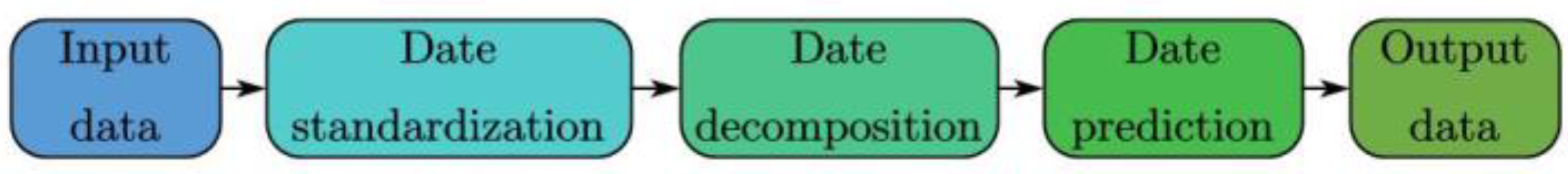
The pre-condition for GRU based on the CEEMDAN–wavelet model is that it has finished its training process. The flow chart is shown in Figure 6.

The steps are as follows:

• Historical data is entered into the model waiting to be used;
• Before using data, the input data needs to be standardized according to formula (22);
• Noise reduction of data using CEEMDAN, and wavelet threshold denoising method is used for high-frequency components;
• The denoised signals are inputted into the trained GRU to get the output value;
• Restoring standardized data.

4.3. Comparative Experiments

The aim of this part is to verify the superiority of the proposed model in predicting future data of the stock market. Consequently, a GRU network without wavelet threshold denoising, an LSTM neural network, a traditional ARIMA, a hybrid CNN-BiLSTM, and an ANN model are selected for comparative experiments to highlight the higher prediction accuracy of our framework model.

4.4. Evaluation Method

In order to compare the correctness of each neural network framework structure for prediction results, we choose four common performance measures to evaluate every model’s accuracy objectively, using a data comparison approach to highlight that the proposed model in this paper has higher accuracy.

Root mean square error (RMSE):

$$RMSE=\sqrt{\frac{{\displaystyle \sum _{i=1}^n{(x_i-y_i)}^2}}{n}}$$

(23)

Mean absolute error (MAE):

$$MAE=\frac{1}{n}{\displaystyle \sum _{i=1}^n\left|{\widehat{y}}_i-y_i\right|}$$

(24)

Coefficient of determination (R²):

$$R^2=\frac{{\displaystyle \sum _{i=1}^n{(x_i-y)}^2}}{{\displaystyle \sum _{i=1}^n{(y_i-y)}^2}}$$

(25)

Mean square error (MSE):

$$MSE=\frac{{\displaystyle \sum _{i=1}^n{(x_i-y_i)}^2}}{n}$$

(26)

4.5. Experimental Result and Comparison

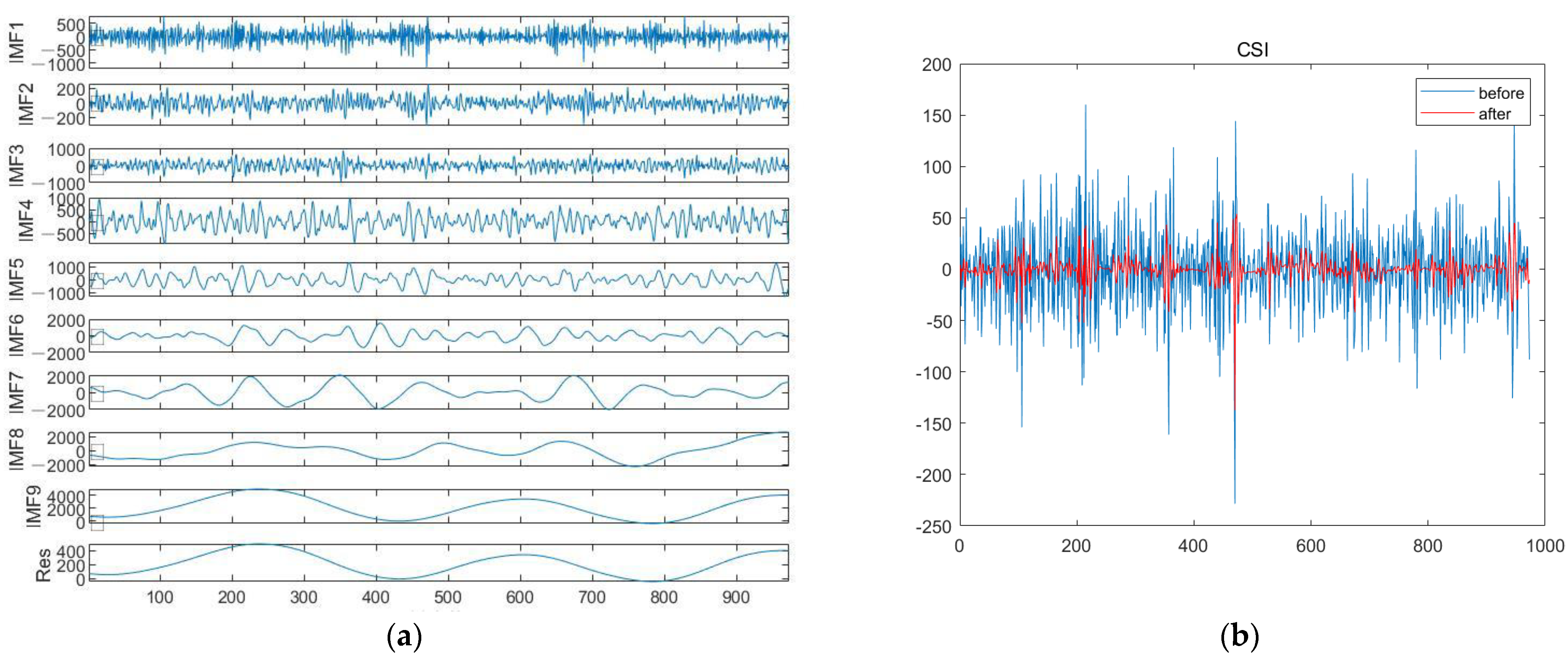
The primary objective was to decompose the data into several sub-signals using CEEMDAN presented in Figure 7a,d and the denoised signals shown in Figure 7b,e.

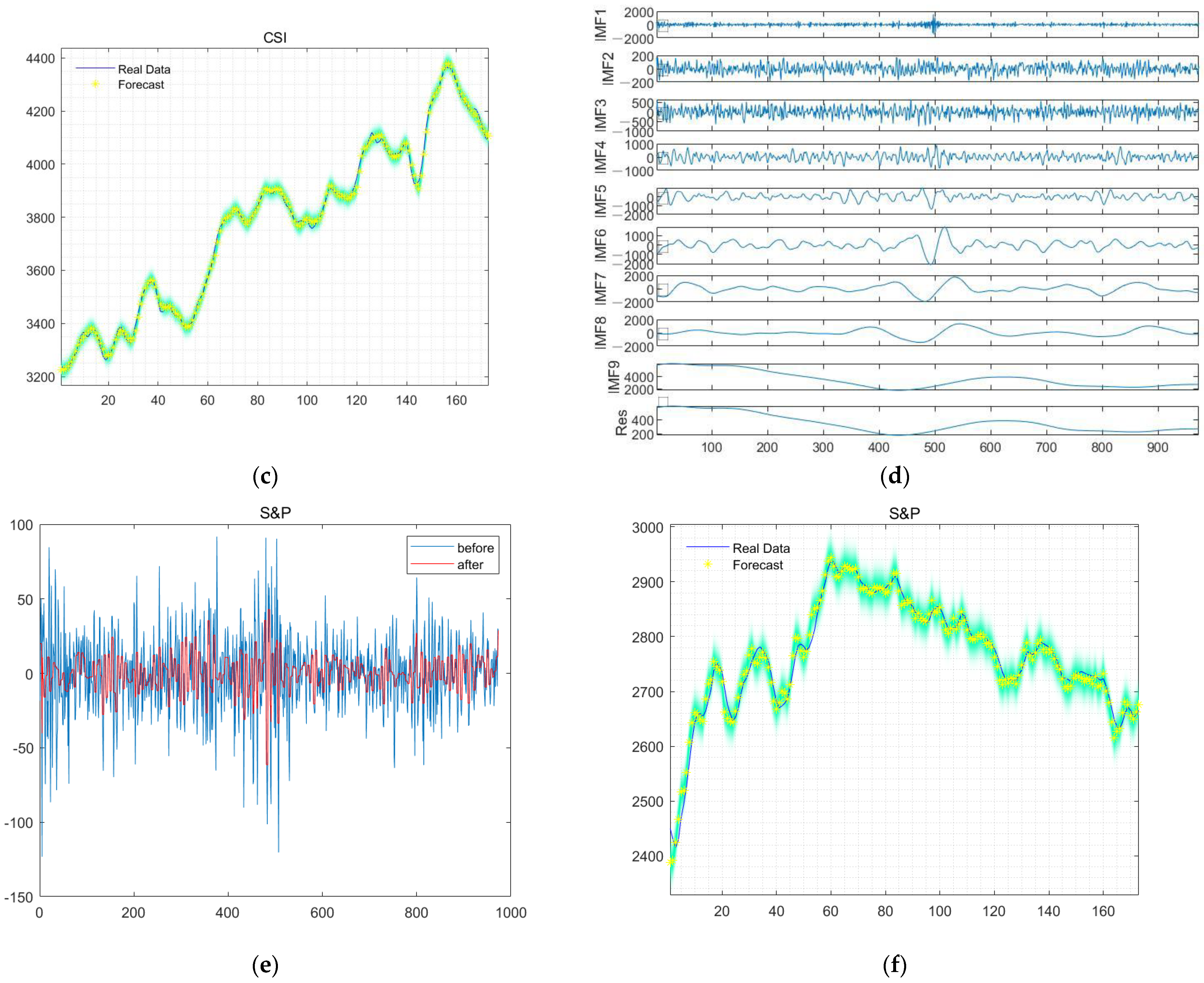
The forecasting curve in Figure 7c,f are plotted using the last 173 days of the test data to illustrate the results of CSI300 and S&P500.

5. Discussion

Figure 7c,f show plots of the actual versus predicted values of the model predicting future movements of the CSI and S&p500 data, respectively.

Table 1. Comparison between proposed network structure and other neural networks based on CSI300.

Model	RMSE	MSE	R2	MAE
GRU based on CEEMDAN–wavelet	12.99	168.89	0.994	10.63
LSTM	18.14	329.06	0.98	15.15
ARIMA	49.376	2437.98	0.79	37.8
GRU	17.07	291.37	0.986	11.96
CNN-BiLSTM	20.14	405.62	0.91	13.68
ANN	22.47	504.90	0.87	14.59

and

Table 2. Comparison between proposed network structure and other neural networks based on S&P500.

Model	RMSE	MSE	R2	MAE
GRU based on CEEMDAN–wavelet	22.27	496.07	0.991	17.39
LSTM	26.34	693.79	0.97	16.544
ARIMA	27.74	769.68	0.94	19.32
GRU	23.51	552.99	0.97	21.23
CNN-BiLSTM	24.28	589.52	0.96	19.87

show that the differential value between the denoised GRU and the non-denoised GRU is 0.008 and 0.019 in the $R^2$ in CSI and S&P, respectively, and both $R^2$ of denoised GRU reach above 0.99, which indicates that the denoised GRU model has a great advantage in the goodness of fit.

In order to select the optimum model, we did ten experiments for the significance analysis test and obtained ten sets of MSE and MAE of the six models. Since the ten sets of MSE and MAE of ARIMA did not have any variation and the mean values were 769.69 and 19.32, which were significantly larger than GRU based on CEEMDAN–wavelet, we found GRU based on CEEMDAN–wavelet is better than ARIMA.

In our study, GRU based on CEEMDAN–wavelet was used as the treatment group model. The LSTM, GRU, and CNN-BiLSTM are compared with GRU based on CEEMDAN–wavelet in turn in a two-by-two t-test, using as the experimental group models. We know that the p-value of the t-test is less than 0.05; in other words, there is a significant difference between the means of the values taken by the two models on this indicator.

Table 3. The MSE significance analysis based on CSI300.

Control Model	Test Model	p Value of t-Test	Mean Value
GRU based on CEEMDAN–wavelet (303.10)	LSTM	0.34	321.60
	GRU	0.01	380.81
	CNN-BiLSTM	2.08 × 10−7	691.78
	ANN	2.51 × 10−6	526.46

and

Table 4. The MAE significance analysis based on CSI300.

Control Model	Test Model	p Value of t-Test	Mean Value
GRU based on CEEMDAN–wavelet (13.70)	LSTM	0.14	14.32
	GRU	0.008	15.38
	CNN-BiLSTM	2.89 × 10−8	20.09
	ANN	0.01	15.21

selected ten experiments of CSI300 to study the significance analysis of MSE and MAE. The mean value of MSE for GRU based on CEEMDAN–wavelet is 303.10 and the mean value of MAE is 13.70. From Table 3 and Table 4, it is concluded that the p-values of t-tests of GRU, CNN-BiLSTM, and ANN on MSE and MAE are less than 0.05, i.e., there is a significant difference in the mean values of these three models on MSE and MAE. In addition, according to the mean values of MSE and MAE obtained by the ten experiments conducted, the mean values of MSE and MAE of GRU based on CEEMDAN–wavelet are the smallest; so, we conclude that GRU based on CEEMDAN–wavelet is superior to the other three models. For LSTM, even though its p-value of the t-test is larger than 0.05, since its mean values of MSE and MAE are larger than those of GRU based on CEEMDAN-wavelet, we conclude that GRU based on CEEMDAN–wavelet is superior to LSTM.

Similarly,

Table 5. The MSE significance analysis based on S&P500.

Control Model	Test Model	p Value of t-Test	Mean Value
GRU based on CEEMDAN–wavelet (162.85)	LSTM	3.11 × 10−11	627.12
	GRU	1.99 × 10−5	477.31
	CNN-BiLSTM	6.07 × 10−5	684.32
	ANN	1.82 × 10−10	700.76

and

Table 6. The MAE significance analysis based on S&P500.

Control Model	Test Model	p Value of t-Test	Mean Value
GRU based on CEEMDAN–wavelet (9.18)	LSTM	9.41 × 10−11	19.09
	GRU	2.37 × 10−5	16.29
	CNN-BiLSTM	1.06 × 10−4	20.31
	ANN	1.91 × 10−9	19.77

represent the ten experiments of S&P500 to study the significance analysis of MSE and MAE. The mean value of MSE for GRU based on CEEMDAN–wavelet is 162.85 and the mean value of MAE is 9.18. From Table 5 and Table 6, it is concluded that the four models of LSTM, GRU, CNN-BiLSTM, and ANN have significant differences in MSE and there is a significant difference in the mean values of the values taken on MAE. The mean values of MSE and MAE for GRU based on CEEMDAN–wavelet are the smallest, so we also believe that GRU based on CEEMDAN–wavelet can outperform the other four models.

Overall, by significance analysis, we conclude that GRU based on CEEMDAN–wavelet is optimum in comparison with the other five models.

6. Conclusions

In this paper, we propose a novel framework combining gated recurrent unit (GRU) neural networks and complete ensemble empirical modal decomposition of adaptive noise (CEEMDAN) to predict stock indices with more accuracy, where the wavelet threshold method is specifically used to denoise high-frequency noise in sub-signals in order to exclude interference noise for future data prediction. We first evaluate the proposed GRU-CEEMDAN–wavelet model with selected representative datasets from the S&P 500 and CSI 300 index closing prices. Meanwhile, we compare the improved model with the traditional ARIMA model and several modified neural network models applying different gate structures. After the verification of various evaluation indicators, the results show that the model is indeed better than the traditional model in terms of forecasting results.

However, financial markets are subject to human interference. We only have four-dimensional features for prediction. The personal behavior of any oligarchic firm or star investor may later lead to volatility in the financial market, and this human factor related to sentiment is not predictable by machine models and is completely random. Therefore, subsequent research wants to extract news keywords and sentiment analysis (e.g., a news article that the program can grab in the first place, and perform semantic analysis and sentiment judgments contained therein. If it is positively favorable, it will be added to the neural network prediction we build as a positive sentiment factor. Together, as a hybrid algorithm, it determines the price direction of the financial market.