
Shapley Values as a Strategy for Ensemble Weights Estimation


Abstract
:1. Introduction
2. Related Work
3. Methods
3.1. Base Learners
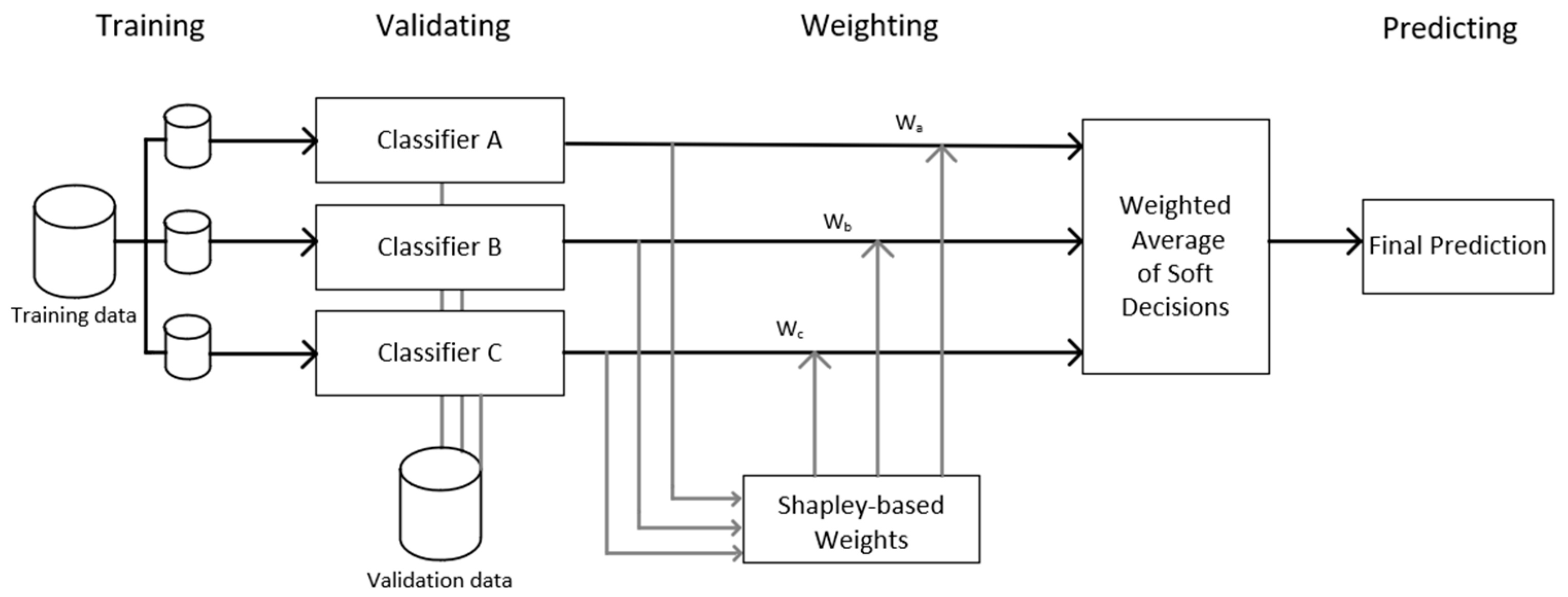
3.2. Weighting Strategies
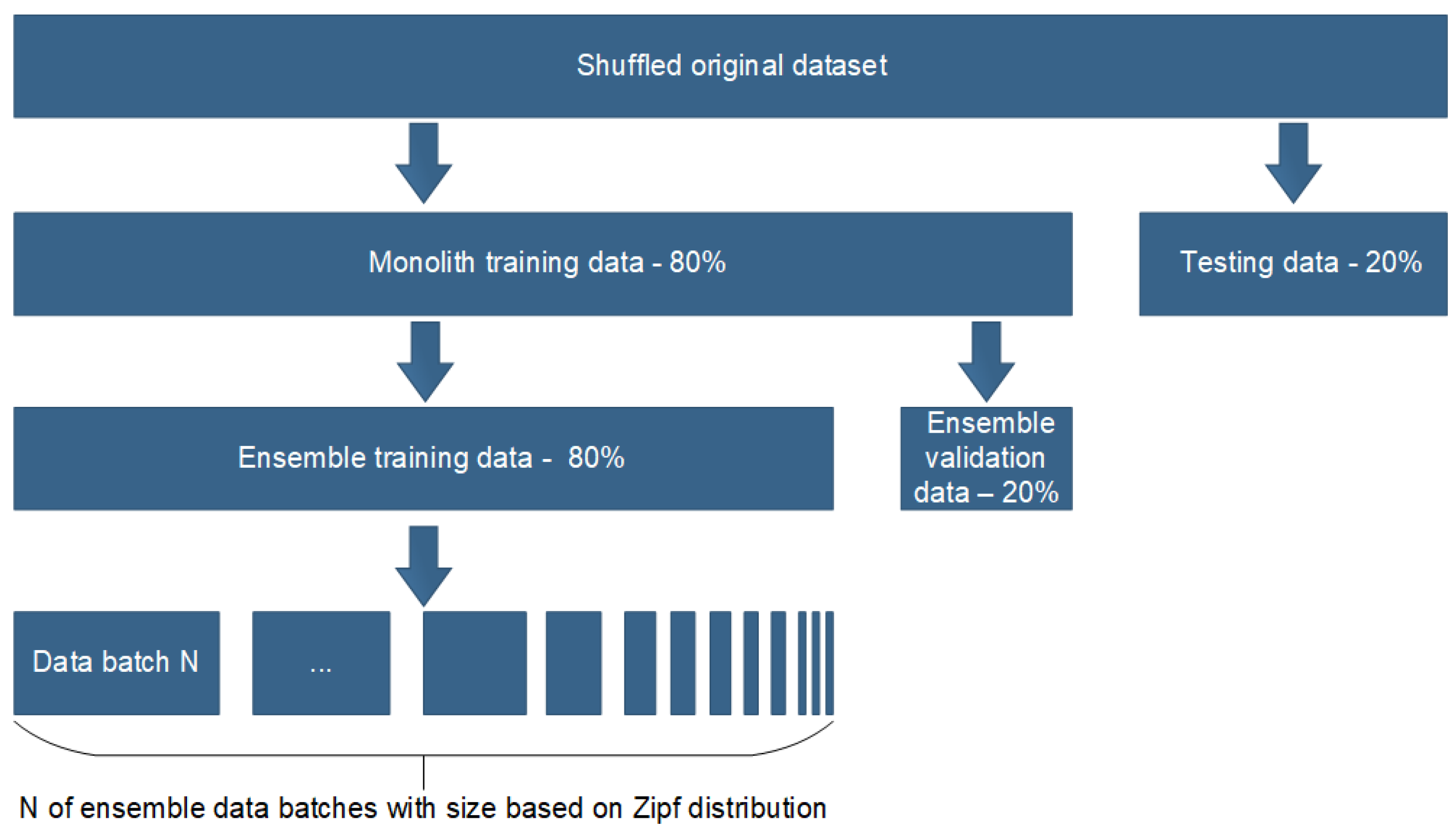
3.3. Data Preparation
3.4. Evaluation Scheme
3.5. Performance Comparison
4. Results and Analysis
4.1. Experimental Setup
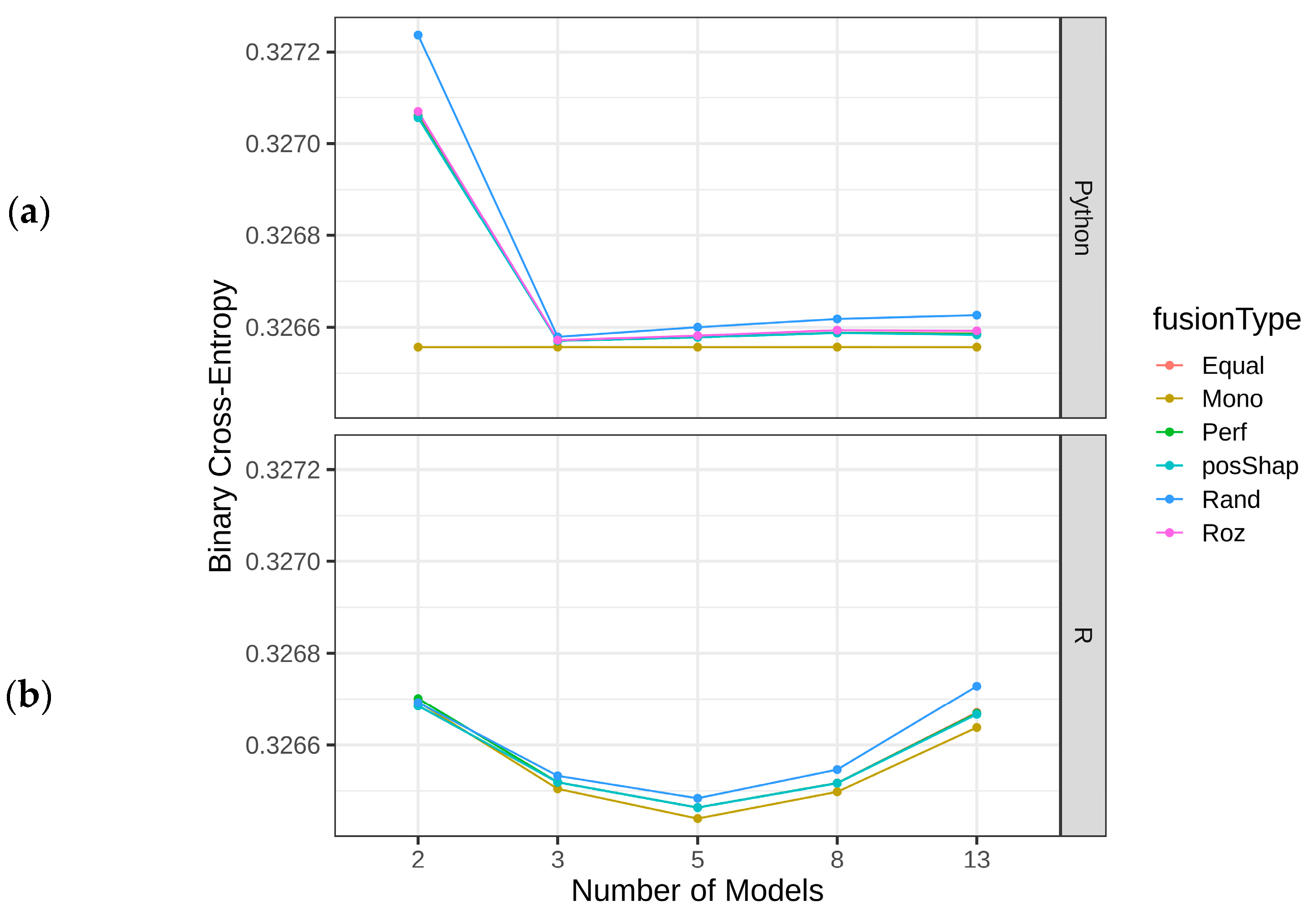
4.2. Experimental Results
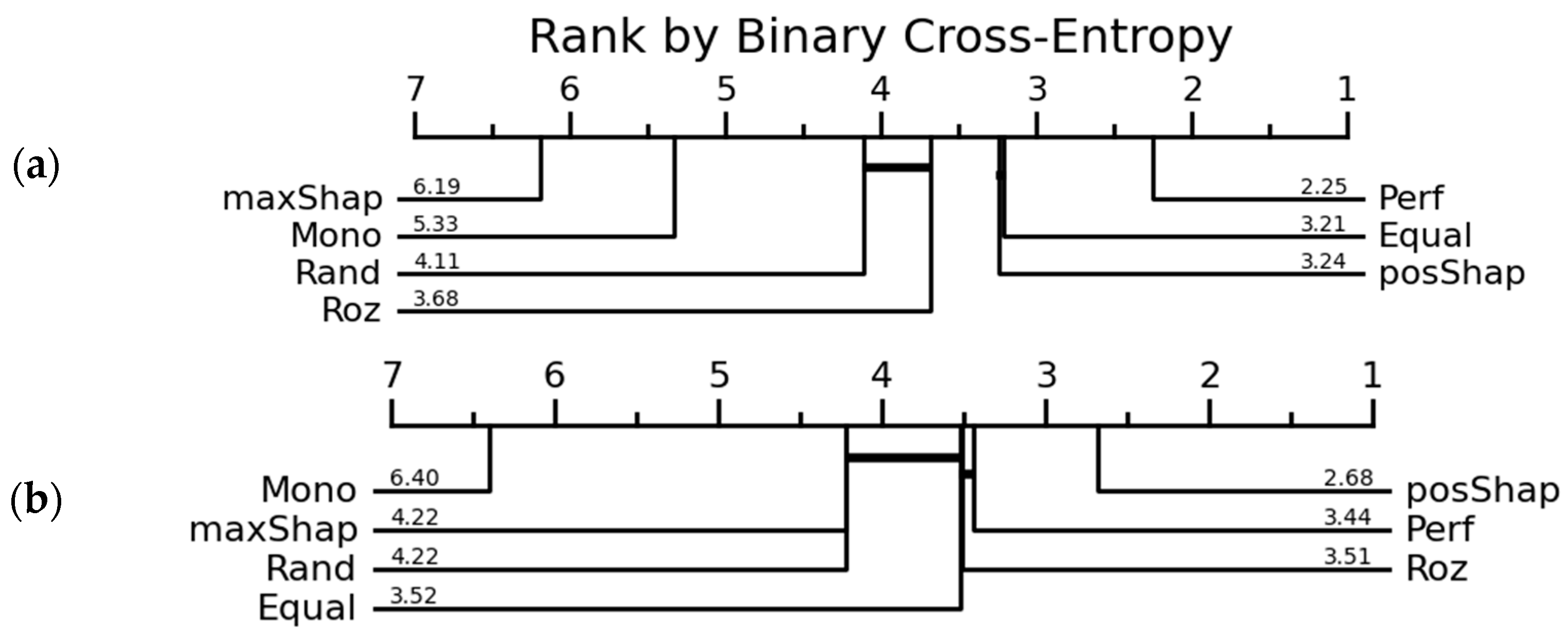
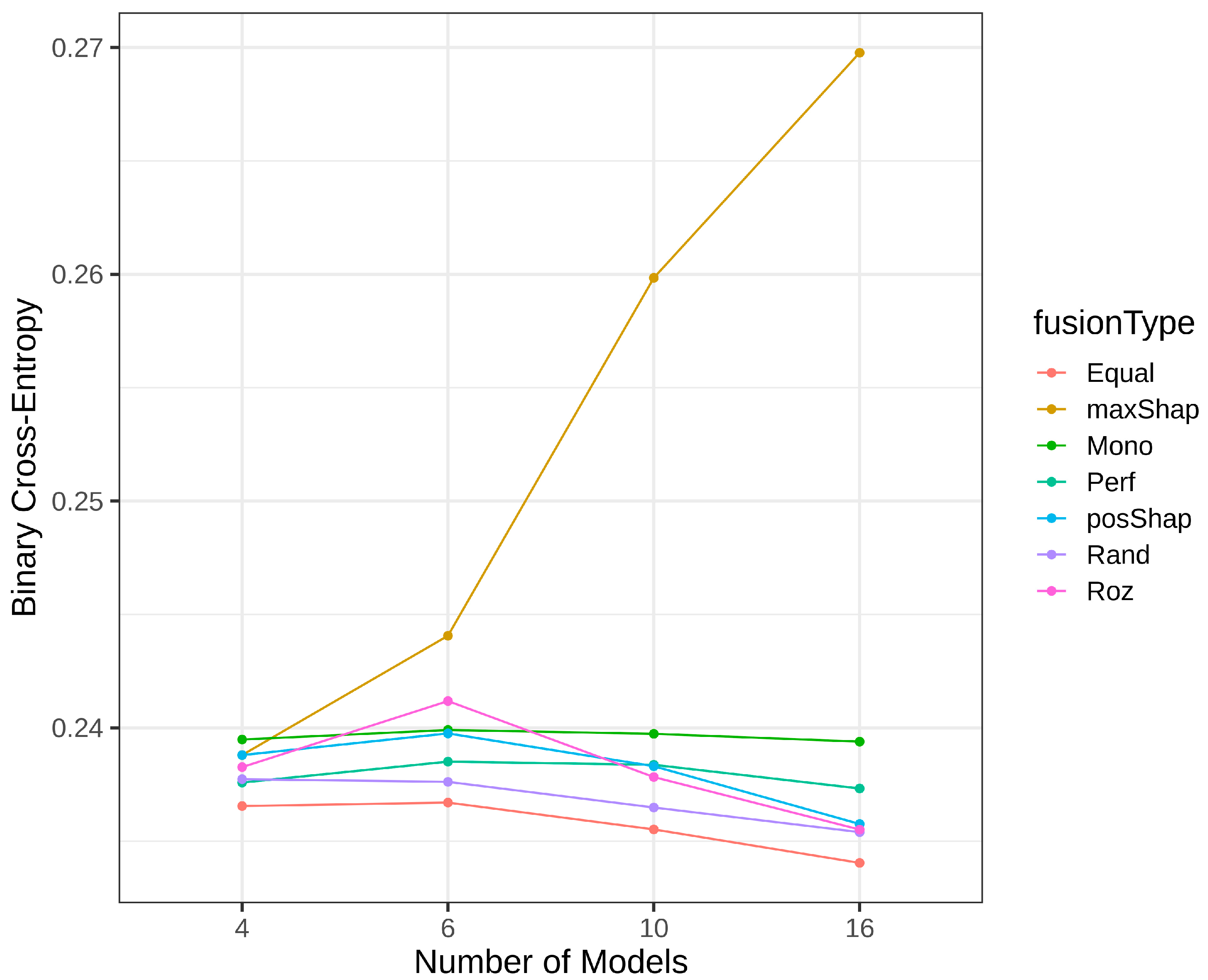
4.3. Results of Homogeneous Model Ensembles
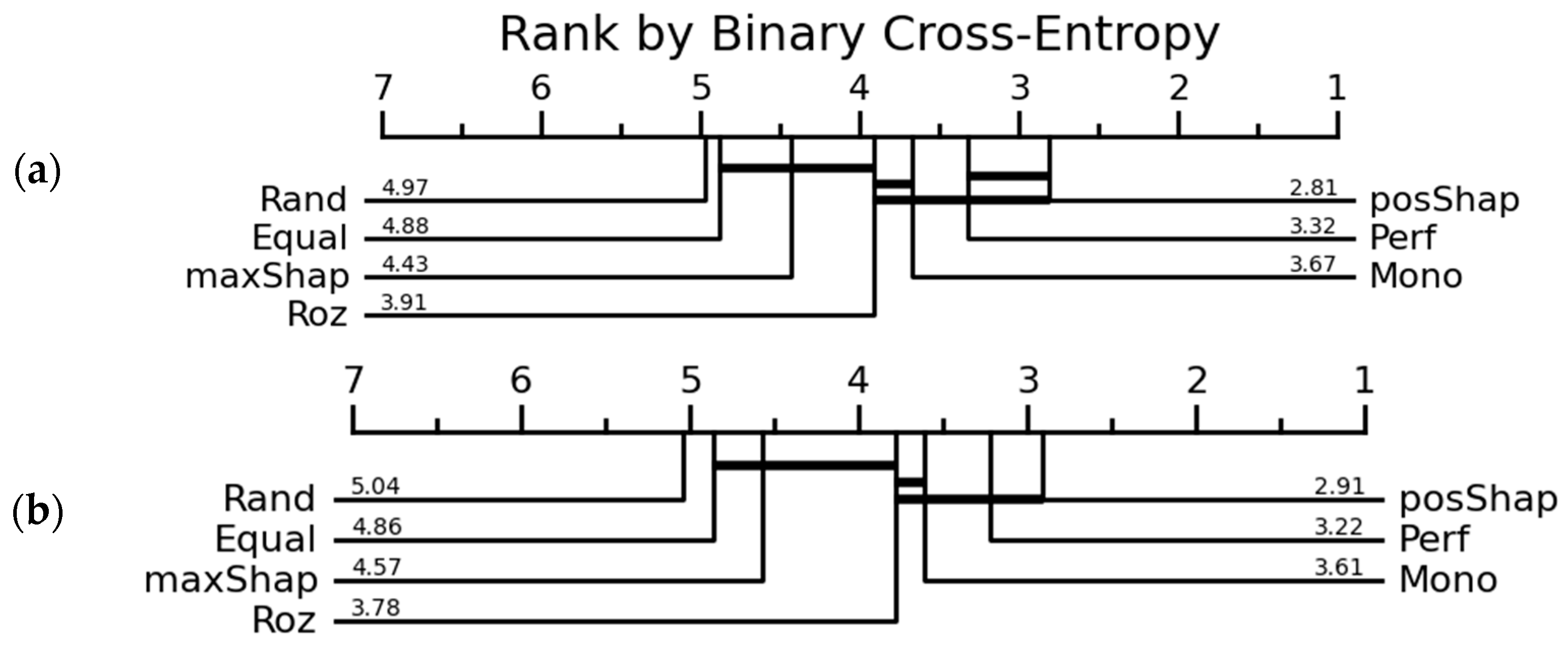
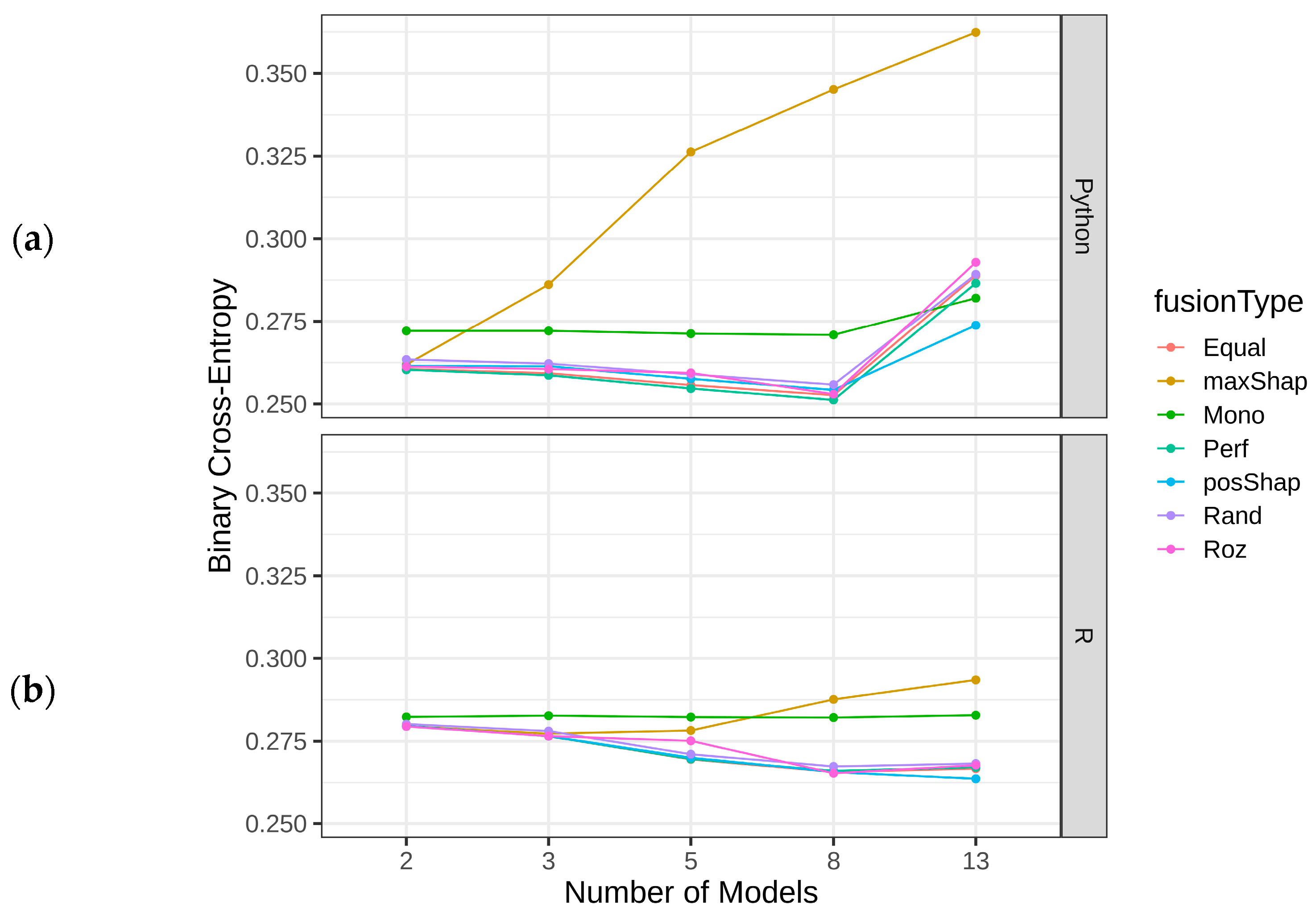
4.4. Heterogenous Ensembles
5. Discussion
6. Conclusions
Author Contributions
Funding
Informed Consent Statement
Data Availability Statement
Conflicts of Interest
References
- Vopson, M.M. The information catastrophe. AIP Adv. 2020, 10, 085014. [Google Scholar] [CrossRef]
- Li, T.; Sahu, A.K.; Talwalkar, A.; Smith, V. Federated learning: Challenges, methods, and future directions. IEEE Signal Process. Mag. 2020, 37, 50–60. [Google Scholar] [CrossRef]
- Schapire, R.E. The strength of weak learnability. Mach. Learn. 1990, 5, 197–227. [Google Scholar] [CrossRef] [Green Version]
- González, S.; García, S.; Del Ser, J.; Rokach, L.; Herrera, F. A practical tutorial on bagging and boosting based ensembles for machine learning: Algorithms, software tools, performance study, practical perspectives and opportunities. Inf. Fusion 2020, 64, 205–237. [Google Scholar] [CrossRef]
- Fan, W.; Stolfo, S.J.; Zhang, J. The application of AdaBoost for distributed, scalable and on-line learning. In Proceedings of the Fifth ACM SIGKDD International Conference on Knowledge Discovery and Data Mining, San Diego, CA, USA, 15–18 August 1999. [Google Scholar]
- Fern, A.; Givan, R. Online ensemble learning: An empirical study. Mach. Learn. 2003, 53, 71–109. [Google Scholar] [CrossRef] [Green Version]
- Street, W.N.; Kim, Y. A streaming ensemble algorithm (SEA) for large-scale classification. In Proceedings of the Seventh ACM SIGKDD International Conference on Knowledge Discovery and Data Mining, San Francisco, CA, USA, 26 August 2001. [Google Scholar]
- Wang, H.; Fan, W.; Yu, P.S.; Han, J. Mining concept-drifting data streams using ensemble classifiers. In Proceedings of the Ninth ACM SIGKDD International Conference on Knowledge Discovery and Data Mining, Washington, DC, USA, 24 August 2003. [Google Scholar]
- Kolter, J.Z.; Maloof, M.A. Dynamic weighted majority: An ensemble method for drifting concepts. J. Mach. Learn. Res. 2007, 8, 2755–2790. [Google Scholar]
- Bowser, A.; Wiggins, A.; Shanley, L.; Preece, J.; Henderson, S. Sharing Data While Protecting Privacy in Citizen Science. Interactions 2014, 21, 70–73. [Google Scholar] [CrossRef]
- Verbraeken, J.; Wolting, M.; Katzy, J.; Kloppenburg, J.; Verbelen, T.; Rellermeyer, J.S. A survey on distributed machine learning. ACM Comput. Surv. Csur 2020, 53, 1–33. [Google Scholar] [CrossRef] [Green Version]
- Wei, J.; Dai, W.; Qiao, A.; Ho, Q.; Cui, H.; Ganger, G.R.; Gibbons, P.B.; Gibson, G.A.; Xing, E.P. Managed communication and consistency for fast data-parallel iterative analytics. In Proceedings of the Sixth ACM Symposium on Cloud Computing, Kohala Coast, HI, USA, 27–29 August 2015. [Google Scholar]
- Ma, C.; Li, J.; Shi, L.; Ding, M.; Wang, T.; Han, Z.; Poor, H.V. When federated learning meets blockchain: A new distributed learning paradigm. IEEE Comput. Intell. Mag. 2022, 17, 26–33. [Google Scholar] [CrossRef]
- Tuladhar, A.; Gill, S.; Ismail, Z.; Forkert, N.D. Alzheimer’s Disease Neuroimaging Initiative, Building machine learning models without sharing patient data: A simulation-based analysis of distributed learning by ensembling. J. Biomed. Inform. 2020, 106, 103424. [Google Scholar] [CrossRef] [PubMed]
- Lu, Y.; Huang, X.; Dai, Y.; Maharjan, S.; Zhang, Y. Blockchain and federated learning for privacy-preserved data sharing in industrial IoT. IEEE Trans. Ind. Inform. 2019, 16, 4177–4186. [Google Scholar] [CrossRef]
- Chen, X.; Ji, J.; Luo, C.; Liao, W.; Li, P. When machine learning meets blockchain: A decentralized, privacy-preserving and secure design. In Proceedings of the IEEE International Conference on Big Data (Big Data), Seattle, WA, USA, 10 December 2018. [Google Scholar]
- Xu, R.; Baracaldo, N.; Joshi, J. Privacy-preserving machine learning: Methods, challenges and directions. arXiv 2021, arXiv:2108.04417. [Google Scholar]
- Shapley, L.S. A value for n-person games. In Contributions to the Theory of Games; Princeton University Press: Princeton, NJ, USA, 1953; Volume 2, pp. 307–318. [Google Scholar]
- Rozemberczki, B.; Sarkar, R. The shapley value of classifiers in ensemble games. In Proceedings of the 30th ACM International Conference on Information & Knowledge Management. Virtual Event, Queensland, Australia, 1–5 November 2021. [Google Scholar]
- Drungilas, V.; Vaičiukynas, E.; Ablonskis, L.; Čeponienė, L. Heterogeneous Models Inference Using Hyperledger Fabric Oracles. In Proceedings of the First Blockchain and Cryptocurrency Conference B2C’ 2022, Barcelona, Spain, 9–11 November 2022. [Google Scholar]
- Drungilas, V.; Vaičiukynas, E.; Jurgelaitis, M.; Butkienė, R.; Čeponienė, L. Towards blockchain-based federated machine learning: Smart contract for model inference. Appl. Sci. 2021, 11, 1010. [Google Scholar] [CrossRef]
- Rokach, L. Ensemble Learning: Pattern Classification Using Ensemble Methods; World Scientific: Singapore, 2019. [Google Scholar]
- Sagi, O.; Rokach, L. Ensemble learning: A survey. Wiley Interdiscip. Rev. Data Min. Knowl. Discov. 2018, 8, e1249. [Google Scholar] [CrossRef]
- Dogan, A.; Birant, D. A weighted majority voting ensemble approach for classification. In Proceedings of the 2019 4th International Conference on Computer Science and Engineering UBMK, Samsun, Turkey, 11–15 September 2019; pp. 1–6. [Google Scholar]
- Prodromidis, A.L.; Stolfo, S.J.; Chan, P.K. Effective and efficient pruning of meta-classifiers in a distributed data mining system. Knowl. Discov. Data Min. J. 1999, 32, 1–29. [Google Scholar]
- Shahhosseini, M.; Hu, G.; Pham, H. Optimizing ensemble weights and hyperparameters of machine learning models for regression problems. Mach. Learn. Appl. 2022, 7, 100251. [Google Scholar] [CrossRef]
- Štrumbelj, E.; Kononenko, I. Explaining prediction models and individual predictions with feature contributions. Knowl. Inf. Syst. 2014, 41, 647–665. [Google Scholar] [CrossRef]
- Lundberg, S.M.; Lee, S.I. A unified approach to interpreting model predictions. Adv. Neural Inf. Process. Syst. 2017, 30, 1–10. [Google Scholar]
- Rozemberczki, B.; Watson, L.; Bayer, P.; Yang, H.T.; Kiss, O.; Nilsson, S.; Sarkar, R. The shapley value in machine learning. arXiv 2022, arXiv:2202.05594. [Google Scholar]
- Tang, S.; Ghorbani, A.; Yamashita, R.; Rehman, S.; Dunnmon, J.A.; Zou, J.; Rubin, D.L. Data valuation for medical imaging using Shapley value and application to a large-scale chest X-ray dataset. Sci. Rep. 2021, 11, 1–9. [Google Scholar] [CrossRef]
- Wang, T.; Rausch, J.; Zhang, C.; Jia, R.; Song, D. A principled approach to data valuation for federated learning. Fed. Learn. Priv. Incent. 2020, 12500, 153–167. [Google Scholar]
- Ykhlef, H.; Bouchaffra, D. Induced subgraph game for ensemble selection. Int. J. Artif. Intell. Tools 2017, 26, 1760003. [Google Scholar] [CrossRef]
- Chen, X.; Li, S.; Xu, X.; Meng, F.; Cao, W. A novel GSCI-based ensemble approach for credit scoring. IEEE Access 2020, 8, 222449–222465. [Google Scholar] [CrossRef]
- Dumitrescu, E.; Hué, S.; Hurlin, C.; Tokpavi, S. Machine learning for credit scoring: Improving logistic regression with non-linear decision-tree effects. Eur. J. Oper. Res. 2022, 297, 1178–1192. [Google Scholar] [CrossRef]
- Laaksonen, J.; Oja, E. Classification with learning k-nearest neighbors. In Proceedings of the International Conference on Neural Networks (ICNN’96), Washington, DC, USA, 3–6 June 1996. [Google Scholar]
- Karthik, S.; Bhadoria, R.S.; Lee, J.G.; Sivaraman, A.K.; Samanta, S.; Balasundaram, A.; Chaurasia, B.K.; Ashokkumar, S. Prognostic kalman filter based bayesian learning model for data accuracy prediction. Comput. Mater. Contin 2022, 72, 243–259. [Google Scholar]
- Loh, W.Y. Classification and regression trees. Wiley Interdiscip. Rev. Data Min. Knowl. Discov. 2011, 1, 14–23. [Google Scholar] [CrossRef]
- King, J.E. Binary Logistic Regression. Best Practices in Quantitative Methods; Osborne, Ed.; Jason SAGE Publications, Inc.: Los Angeles, CA, USA, 2008. [Google Scholar]
- Wang, Q.; Ma, Y.; Zhao, K.; Tian, Y. A comprehensive survey of loss functions in machine learning. Ann. Data Sci. 2020, 1–26. [Google Scholar] [CrossRef]
- Roth, A.E. The Shapley Value: Essays in Honor of Lloyd S. Shapley; Cambridge University Press: Cambridge, UK, 1988. [Google Scholar]
- Zhang, Z.; Ho, K.M.; Hong, Y. Machine learning for the prediction of volume responsiveness in patients with oliguric acute kidney injury in critical care. Crit. Care 2019, 23, 112. [Google Scholar] [CrossRef] [PubMed] [Green Version]
- Agarap, A.F. Deep Learning using Rectified Linear Units (ReLU). arXiv 2018, arXiv:1803.08375. [Google Scholar]
- Sergio, M.; Laureano, R.; Cortez, P. Using Data Mining for Bank Direct Marketing: An Application of the CRISP-DM Methodology. In Proceedings of the European Simulation and Modelling Conference-ESM’2011, Guimarães, Portugal, 24–26 October 2011. [Google Scholar]
- Quinlan, J.R. Simplifying decision trees. Int. J. Man-Mach. Stud. 1987, 27, 221–234. [Google Scholar] [CrossRef] [Green Version]
- van Rijn, J.N.; Holmes, G.; Pfahringer, B.; Vanschoren, J. Algorithm selection on data streams. In Proceedings of the Discovery Science: 17th International Conference, Bled, Slovenia, 8–10 October 2014. [Google Scholar]
- Hsieh, K.; Phanishayee, A.; Mutlu, O.; Gibbons, P. The non-iid data quagmire of decentralized machine learning. In Proceedings of the International Conference on Machine Learning, Virtual Event, 12–18 July 2020. [Google Scholar]
- Stripelis, D.; Thompson, P.M.; Ambite, J.L. Semi-synchronous federated learning for energy-efficient training and accelerated convergence in cross-silo settings. ACM Trans. Intell. Syst. Technol. (TIST) 2022, 13, 78. [Google Scholar] [CrossRef]
- Michieli, U.; Ozay, M. Prototype guided federated learning of visual feature representations. arXiv 2021, arXiv:2105.08982. [Google Scholar]
- Arnold, S.; Yesilbas, D. Demystifying the effects of non-independence in federated learning. arXiv 2021, arXiv:2103.11226. [Google Scholar]
- Wadu, M.M.; Samarakoon, S.; Bennis, M. Joint client scheduling and resource allocation under channel uncertainty in federated learning. IEEE Trans. Commun. 2021, 69, 5962–5974. [Google Scholar] [CrossRef]
- Wang, X.; Han, Y.; Wang, C.; Zhao, Q.; Chen, X.; Chen, M. In-edge ai: Intelligentizing mobile edge computing, caching and communication by federated learning. IEEE Netw. 2019, 33, 156–165. [Google Scholar] [CrossRef] [Green Version]
- Zhou, X.; Deng, Y.; Xia, H.; Wu, S.A.; Bennis, M. Time-triggered Federated Learning over Wireless Networks. IEEE Trans. Wirel. Commun. 2022, 21, 11066–11079. [Google Scholar] [CrossRef]
- Critical Difference Diagram with Wilcoxon-Holm Post-Hoc Analysis. Available online: https://github.com/hfawaz/cd-diagram (accessed on 15 March 2023).
- Ismail Fawaz, H.; Forestier, G.; Weber, J.; Idoumghar, L.; Muller, P.A. Deep learning for time series classification: A review. Data Min. Knowl. Discov. 2019, 33, 917–963. [Google Scholar] [CrossRef] [Green Version]
- Friedman, M. A comparison of alternative tests of significance for the problem of m rankings. Ann. Math. Stat. 1940, 11, 86–92. [Google Scholar] [CrossRef]
- Benavoli, A.; Corani, G.; Mangili, F. Should we really use post-hoc tests based on mean-ranks? J. Mach. Learn. Res. 2016, 17, 152–161. [Google Scholar]
- Wilcoxon, F. Individual comparisons of grouped data by ranking methods. J. Econ. Entomol. 1946, 39, 269–270. [Google Scholar] [CrossRef]
- Holm, S. A simple sequentially rejective multiple test procedure. Scand. J. Stat. 1979, 6, 65–70. [Google Scholar]
- The Official Implementation of “The Shapley Value of Classifiers in Ensemble Games” (CIKM 2021). Available online: https://github.com/benedekrozemberczki/shapley (accessed on 10 May 2023).
- Experiment Results for All Tested Ensemble Sizes and Datasets. Available online: https://github.com/HurrisLT/ShapleyWeighting (accessed on 10 May 2023).
- Heaton, J. An empirical analysis of feature engineering for predictive modeling. In Proceedings of the SoutheastCon, Norfolk, VA, USA, 30 March–3 April 2016. [Google Scholar]
- Castro, J.; Gómez, D.; Tejada, J. Polynomial calculation of the Shapley value based on sampling. Comput. Oper. Res. 2009, 36, 1726–1730. [Google Scholar] [CrossRef]
- Maleki, S.; Tran-Thanh, L.; Hines, G.; Rahwan, T.; Rogers, A. Bounding the estimation error of sampling-based Shapley value approximation. arXiv 2013, arXiv:1306.4265. [Google Scholar]
- Uzunoglu, B.; Fletcher, S.J.; Zupanski, M.; Navon, I.M. Adaptive ensemble reduction and inflation. Q. J. R. Meteorol. Soc. A J. Atmos. Sci. Appl. Meteorol. Phys. Oceanogr. 2007, 133, 1281–1294. [Google Scholar] [CrossRef] [Green Version]


| Article | Metrics Used | Shapley Calculation Approach | Application Area |
|---|---|---|---|
| Benedek Rozemberczki [19] | Prediction voting | Expected marginal contributions approximation | Method to quantify the model importance in an ensemble |
| Hadjer Ykhlef [32] | Classifier accuracy | Exact calculations | Ensemble selection method |
| Tianhao Wang [31] | Classifier accuracy | Permutation sampling-based approximation, group testing-based approximation | Method to evaluate data importance in federated learning approaches |
| Xiaohong Chen [33] | Generalized Shapley Choquet integral | Exact calculations | A heterogeneous ensemble classifier for credit risk management |
| Our proposal | Binary cross-entropy | Exact calculations | Ensemble weight selection strategy |
| Data Characteristic | Bank Marketing | BNG-Credit_a |
|---|---|---|
| Initial features | 16 | 15 |
| Categorical features | 10 | 10 |
| Total features | 51 | 33 |
| Total instances | 45,211 | 1,000,000 |
| Classes | 2 | 2 |
| Target class proportion | 0.12 | 0.544 |
| Dataset sources | Bank Marketing [43] | BNG_credit-a [44,45] |
| Model Type | Common Parameters | Implementation-Specific Parameters |
|---|---|---|
| MLR3 LR 1 | E = e × 108 iterations = 25 | singular.ok = True; trace = False |
| PySpark LR 1 | regParam = 0.0; aggregationDepth = 2; threshold = 0.5; elasticNetParam = 0.0; fitIntercept = True | |
| MLR3 DT 2 | maxDepth = 30 minInfoGain = 0.01 | minSplit = 20; maxcompete = 4; maxsurrogate = 5; surrogatestyle = 0; usesurrogate = 2; xval = 10 |
| PySpark DT 2 | minInstancesPerNode = 20; Standardization = False; minWeightFractionPerNode = 0.0; minInstancesPerNode = 1; maxBins = 32; minInfoGain = 0.0; impurity = ‘gini’ |
| Model Type | LR 1 | DT 2 | LR 1 | DT 2 | |||||
|---|---|---|---|---|---|---|---|---|---|
| Dataset | BNG 3 | BNG 3 | Bank 4 | Bank 4 | |||||
| Implementation | Python | R | Python | R | Python | R | Python | R | |
| Weighting Strategy | |||||||||
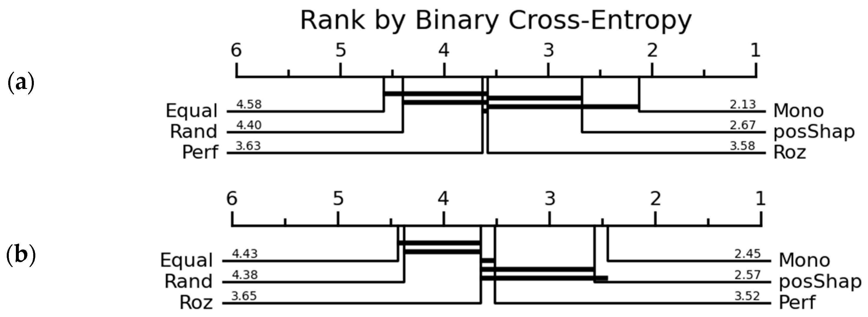
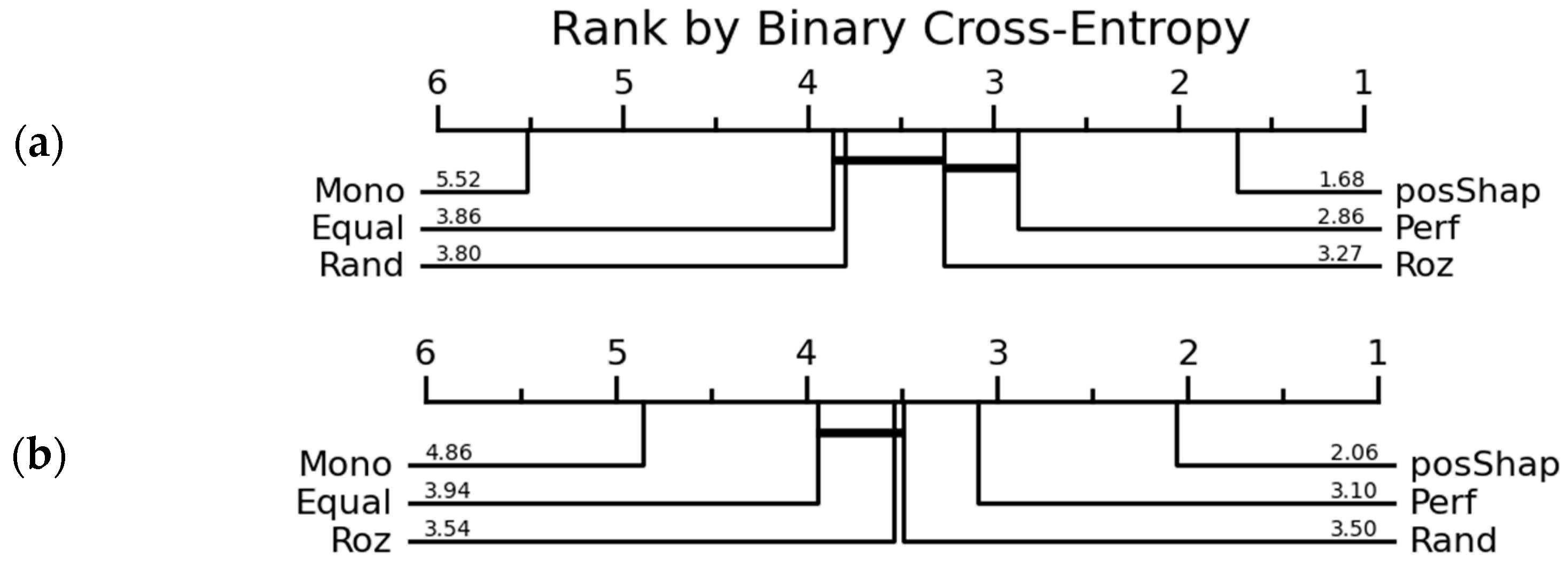
| Mono | 2.13 | 2.45 | 5.52 | 4.86 | 3.67 | 3.61 | 5.33 | 6.40 | |
| Rand | 4.40 | 4.38 | 3.80 | 3.50 | 4.97 | 5.04 | 4.11 | 4.22 | |
| Equal | 4.58 | 4.43 | 3.86 | 3.94 | 4.88 | 4.86 | 3.21 | 3.52 | |
| Perf | 3.63 | 3.52 | 2.86 | 3.10 | 3.32 | 3.22 | 2.25 | 3.44 | |
| Roz | 3.58 | 3.65 | 3.27 | 3.54 | 3.91 | 3.78 | 3.68 | 3.51 | |
| MaxShap | - | - | - | - | 4.43 | 4.57 | 6.19 | 4.22 | |
| PosShap | 2.67 | 2.57 | 1.68 | 2.06 | 2.81 | 2.91 | 3.24 | 2.68 | |
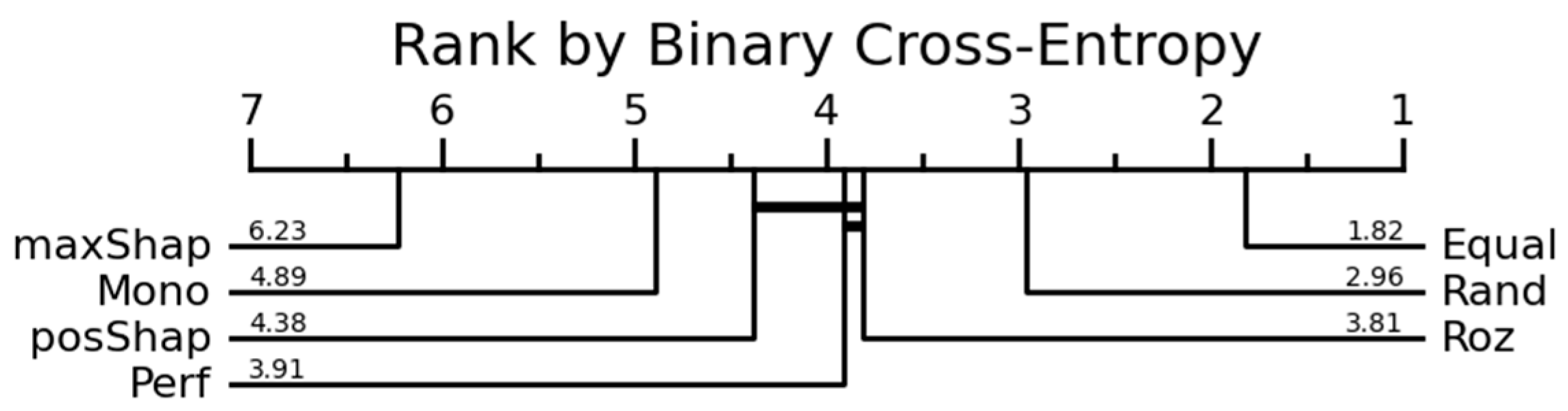
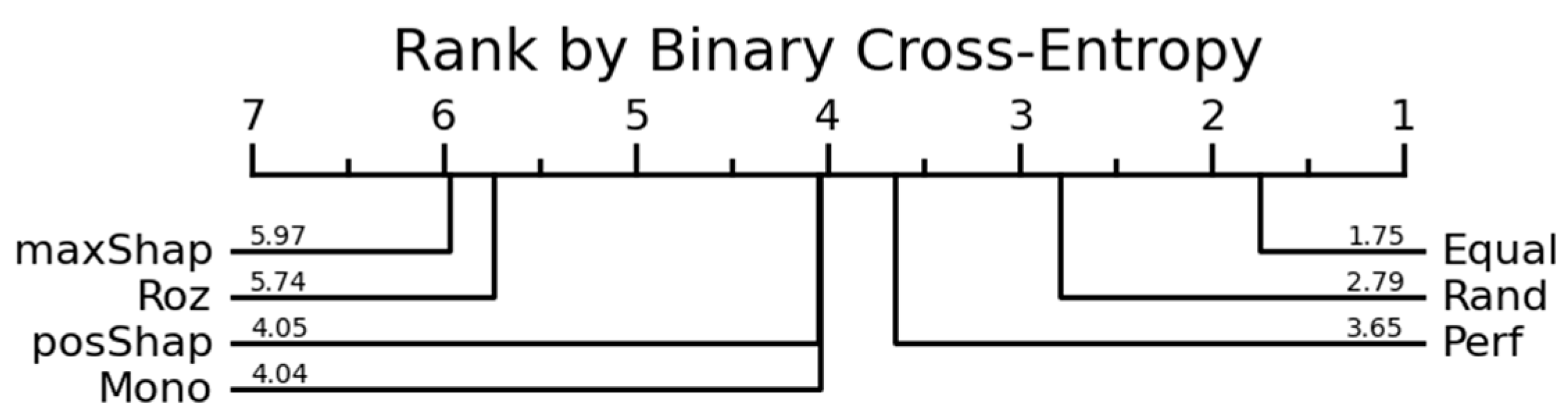
| Dataset | BNG 1 | Bank 2 | ||||
|---|---|---|---|---|---|---|
| Implementation | Python | R | Python | R | ||
| Weighting Strategy | ||||||
| Mono | 5.99 | 1 | 4.89 | 4.04 | ||
| Rand | 3.54 | 3.79 | 2.96 | 2.79 | ||
| Equal | 3.26 | 3.88 | 1.82 | 1.75 | ||
| Perf | 3.20 | 3.53 | 3.91 | 3.65 | ||
| Roz | 3.09 | 5.50 | 3.81 | 5.74 | ||
| MaxShap | - | - | 6.23 | 5.97 | ||
| PosShap | 1.92 | 3.29 | 4.38 | 4.05 | ||
Disclaimer/Publisher’s Note: The statements, opinions and data contained in all publications are solely those of the individual author(s) and contributor(s) and not of MDPI and/or the editor(s). MDPI and/or the editor(s) disclaim responsibility for any injury to people or property resulting from any ideas, methods, instructions or products referred to in the content. |
© 2023 by the authors. Licensee MDPI, Basel, Switzerland. This article is an open access article distributed under the terms and conditions of the Creative Commons Attribution (CC BY) license (https://creativecommons.org/licenses/by/4.0/).
Share and Cite
Drungilas, V.; Vaičiukynas, E.; Ablonskis, L.; Čeponienė, L. Shapley Values as a Strategy for Ensemble Weights Estimation. Appl. Sci. 2023, 13, 7010. https://doi.org/10.3390/app13127010
Drungilas V, Vaičiukynas E, Ablonskis L, Čeponienė L. Shapley Values as a Strategy for Ensemble Weights Estimation. Applied Sciences. 2023; 13(12):7010. https://doi.org/10.3390/app13127010
Chicago/Turabian StyleDrungilas, Vaidotas, Evaldas Vaičiukynas, Linas Ablonskis, and Lina Čeponienė. 2023. "Shapley Values as a Strategy for Ensemble Weights Estimation" Applied Sciences 13, no. 12: 7010. https://doi.org/10.3390/app13127010