A Low-Complexity Deep Learning Model for Predicting Targeted Sequencing Depth from Probe Sequence

Abstract

Targeted sequencing has been widely utilized for genomic molecular diagnostics and the emerging DNA data storage paradigm. However, the probe sequences used to enrich regions of interest have different hybridization kinetic properties, resulting in poor sequencing uniformity and setting limitations for the large-scale application of the technology. Here, a low-complexity deep learning model is proposed for prediction of sequencing depth from probe sequences. To capture the representation of probe and target sequences, we utilized a sequence-encoding model that incorporates k-mer and word embedding techniques, providing a streamlined alternative to the intricate computations involved in biochemical feature analysis. We employed bidirectional long short-term memory (Bi-LSTM) to effectively capture both long-range and short-range interactions within the representation. Furthermore, the attention mechanism was adopted to identify pivotal regions in the sequences that significantly influence sequencing depth. The ratio of the predicted sequencing depth to the actual sequencing depth was in the interval of 1/3—3 as the evaluation metric of model accuracy. The prediction accuracy was 94.3% in the human single-nucleotide polymorphism (SNP) panel and 99.7% in the synthetic DNA information storage sequence (SynDNA) panel. Our model substantially reduced data processing time (from 334 min to 4 min of CPU time in the SNP panel) and model parameters (from 300 k to 70 k) compared with the baseline model.

1. Introduction

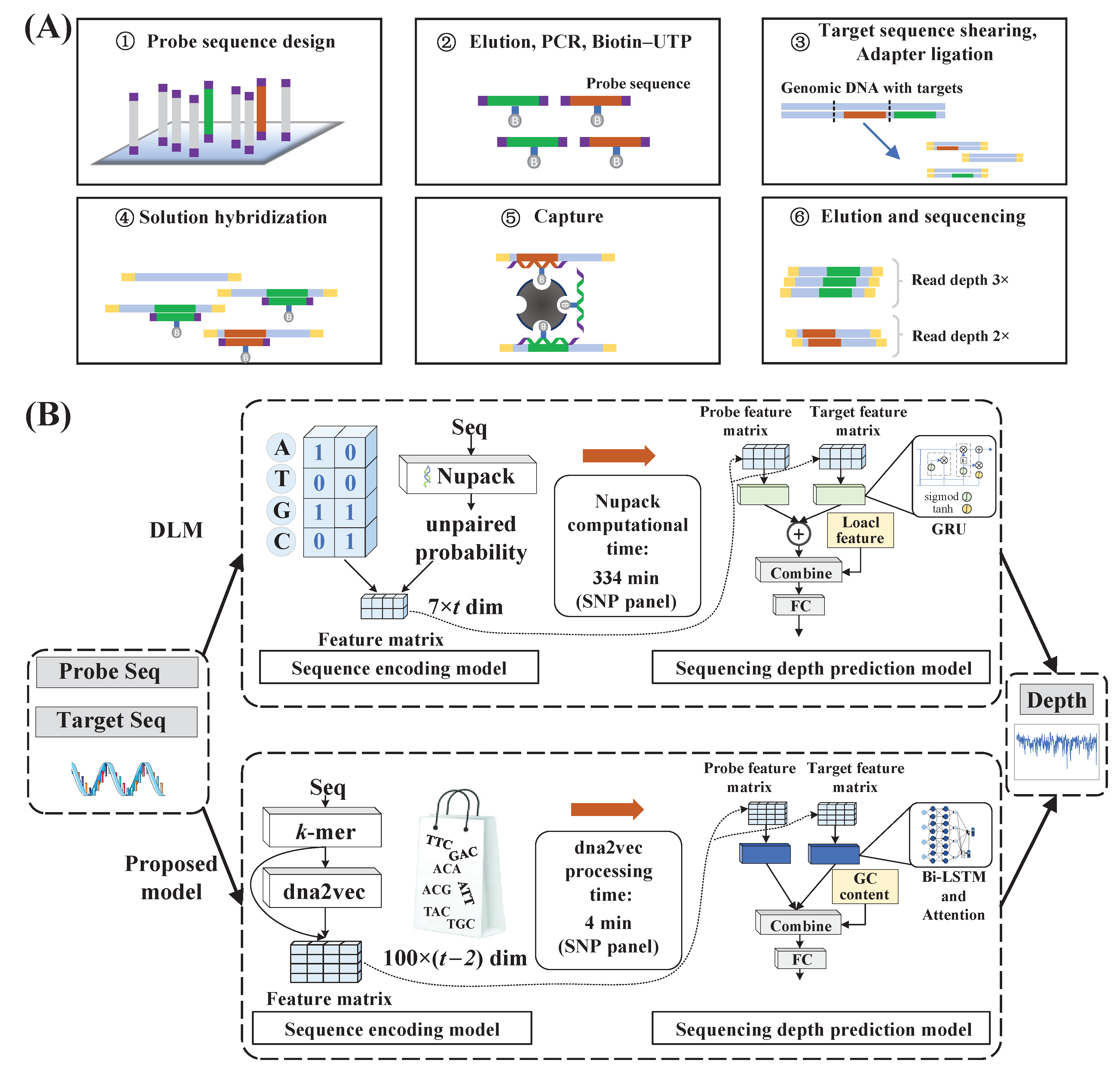
With the development of next-generation sequencing (NGS) technology, its massively parallel sequencing ability and high analytical sensitivity have made it an increasingly prevalent tool in diverse fields, such as population genomics, cancer or disease genetics, and DNA data storage [1,2,3,4]. In the realm of genome ecology, there are three main types of NGS sequencing, encompassing targeted sequencing, whole-exome sequencing, and whole-genome sequencing. Targeted sequencing uses probes to enable the process of enriching and sequencing specific regions of DNA [5], with the work flow shown in Figure 1A. In next-generation sequencing, probe sequences enable researchers to focus their sequencing efforts on areas of interest by targeting specific genomic regions [6], thereby reducing the sequencing time and cost associated with analyzing the entire genome. However, the hybridization kinetic properties of the probe structure lead to uneven enrichment efficiency, which results in increased sequencing costs. Therefore, modeling the impact of probe character on enrichment efficiency can aid in the design of probe sequences that ensure a uniform coverage of sequencing depth.

In recent years, some traditional methods based on experience with DNA structure and biochemistry have been presented to optimize probe sequences for specific hybridization between probe and target sequences [7,8]. Several studies have shown that the traditional methods are labor-intensive and poorly generalized [9]. In recent years, deep learning approaches have leveraged diverse neural network architectures to autonomously extract weakly correlated features from large datasets, leading to significant breakthroughs in various scientific domains, including natural language processing (NLP) and computer vision (CV) [10,11,12,13]. The latest research indicates that deep learning has been successfully applied in the field of bioinformatics for emerging tasks (e.g., protein structure prediction and medical image analysis) [14,15,16,17]. In the prediction of sequencing depth for targeted sequencing, the short-range and long-range interactions in the sequence can lead to the formation of different secondary structures, affecting the kinetic nature of the hybridization reaction and the efficiency of probe capture. This interaction phenomenon between different regions can be trapped by the recurrent neural network (RNN). The large NGS dataset also offers the possibility of using deep learning to solve this problem.

A deep learning model (DLM) was introduced to predict sequencing depth [9]. The unpaired probability of each nucleotide in all possible secondary structures of the probe sequence was calculated using Nupack as the local feature [18]; then, the standard free energy of the probe sequence, the target sequence, and the molecule after hybridization of the probe sequence were calculated as global features. The local feature of each nucleotide with the nucleotide chemical identity (NCP) was used to complete the process of encoding the sequence into the matrix. Four gate-recurrent units (GRUs) were utilized to process the probe and target sequences separately. The processing results were combined with global features and fed into the fully connected neural network to accomplish sequencing depth prediction.

Although the existing deep learning model is effective at predicting the sequencing depth of probe sequences, it suffers from several limitations. (1) The process of using Nupack to calculate the unpaired probability of each nucleotide is time-consuming. Therefore, it is possible to use only a few local features of the sequence, which are derived directly from the sequence itself, avoiding the need for a complex and uncertain thermodynamic calculation process. (2) NCP-based sequence encoding leads to less information input because it only describes the characteristics of the sequence without considering the dependence of nucleotides in the sequence. Thus, the representation of sequences can be achieved with higher-dimensional matrices. dna2vec enables the application of NLP techniques to DNA sequences by using sequence information to acquire the k-mer distributed representation [19]. (3) Although the attention mechanism has been widely applied in bioinformatics and possesses a better prediction ability, it has not yet been commonly applied in the field of sequencing depth prediction, so it can be introduced to improve the accuracy of the sequencing depth prediction.

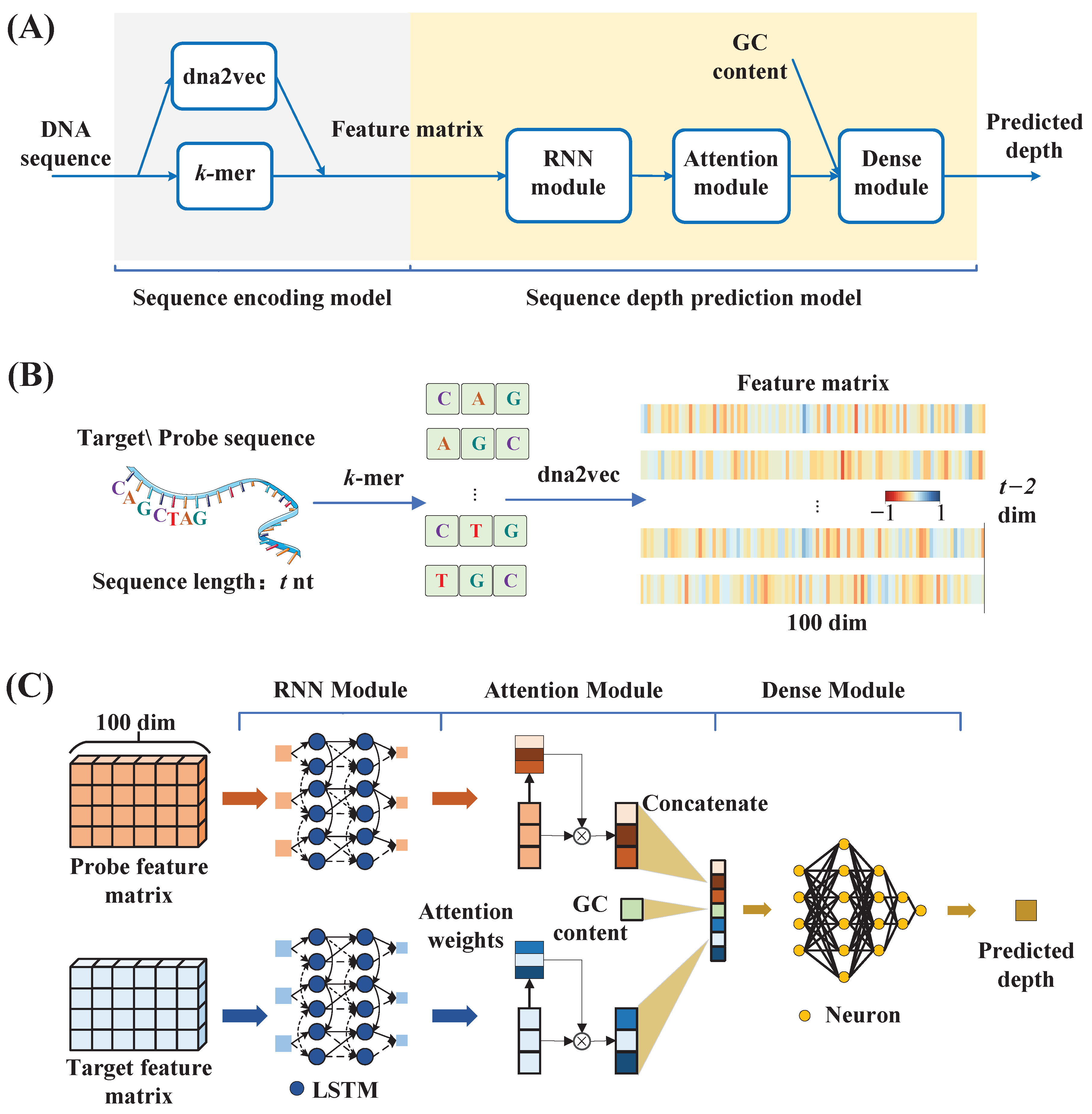
To overcome these limitations, we proposed a low-complexity deep learning model to predict the sequencing depth of probe sequences in targeted sequencing. Specifically, in this model, the target and probe sequences were first split into k-mer word vector representations using k-mer processing. Subsequently, the association information between different k-mer word vectors was extracted from the probe sequences using the dna2vec model to obtain the high-dimensional vector representation of the k-mer word vectors. The sequences were transformed into distributed representations based on the different high-dimensional vector representation combinations. Then, the Bi-LSTM was utilized to process the sequences sequentially according to base positions, and interactions between adjacent bases (short-range interactions), as well as interactions between bases that were far apart (long-range interactions), were captured as output for subsequent processing. Later, the attention mechanism was employed to process the output of the Bi-LSTM. Its ability to represent the different effects of nucleotides at different positions on sequencing depth by setting different weights allowed the model to selectively focus on positions that were more important for sequencing depth prediction. Finally, the predicted log sequencing depth was derived through a deep neural network. Figure 1B provides an overview of the DLM and the proposed sequencing depth prediction model.

2. Materials and Methods

2.1. Datasets

The NGS experiment generated a large number of sequencing datasets, and the baseline dataset used in this paper was the same as the DLM, including three panels of SNP, long non-coding RNA (lncRNA) [20], and SynDNA. The SNP panel fastq file contained 21,857,262 reads, and the fasta file contained 39,145 probe sequences. By using the conventional read alignment tool BWA to match the fastq file and counting the matched values [21], a dataset of 38,040 probes was obtained after excluding 1105 probes with zero matched reads. The lncRNA panel consisted of 1966 probes with reads secured by using BWA to match the fastq file. The SynDNA panel included 7215 probes with reads gained using BWA to match the fastq file. Histograms of GC content and log sequencing depth for the three sets of probe sequences are shown in Figure 2, which shows that the SynDNA panel has a more concentrated GC content of around 0.5 and a tighter distribution in sequencing depth compared with the SNP and lncRNA panels. The figure also indicates that the distribution of GC content showed a correlation with the distribution of sequencing depth [22,23].

2.2. Sequence Encoding Model

In this study, the next-generation sequencing depth was predicted using a new deep learning approach. A flow chart of our new method is shown in Figure 3A. From the deep learning perspective, the process of predicting the sequencing depth from probe sequences could be regarded as a regression task. Since sequences could not be used directly as input to a neural network, they needed to be transformed into vector representations. The sequence encoding process is shown in Figure 3B. The input sequence and sequencing depth were treated as ${\left\{{\mathbf{X}}^j,y^j\right\}}_{j=1}^n$ using k-mer and dna2vec, where ${\mathbf{X}}^j$ represents the embedded probe sequences, $y^j$ represents the probe sequencing depth, and n signifies the number of sequences in the dataset.

First, the k-mer processing method, which is commonly used in sequence analysis and processing, was selected to segment the target sequence and probe sequence, where mer represents the monomer unit, and k indicates segmentation into k bases in length. Setting different step sizes (s) yielded k-mer segmentation results with different intervals. Taking a sequence as an example, the step size (s) was set as 1, and the value of k was set to 3. Therefore, a probe sequence (D) with a length of t bp could be expressed as

$$D=n_1{n}_2{n}_3\dots n_j\dots n_t,(n_j\in \{A,T,C,G\}),$$

(1)

where $n_j$ represents the nucleotide in the j-th position. The k-mer processing method was utilized to split it into $t-2$ subsequences with a length of 3 mer. Then, these $t-2$ subsequences were regarded as the words that made up the sentence of the DNA sequence, which was described as

$$S=\left\{N_1,N_2,\dots ,N_j,\dots ,N_{t-2}\right\},$$

(2)

where $N_j$ represents the subsequence at the j-th position $\left\{n_j{n}_{j+1}{n}_{j+2}\right\}$ taken from $\left\{AAA\right\}$, $\left\{AAC\right\}$, $\left\{AAG\right\},\dots ,\left\{TTT\right\}$.

Then, the dna2vec method was applied to generate word vector representations for each 3-mer subsequence obtained through k-mer processing. The dna2vec method is an improvement of word2vec using skip-gram [24,25], which predicted the occurrence probability of the target subsequence and generated its word vector based on all sequence correlations. Each subsequence ($N_j$) was transformed into a 100-dimensional vector (${\mathbf{x}}_j$). The sequence (D) was converted into a distributed representation ($\mathbf{X}$) as follows

$$\mathbf{X}=\left[{\mathbf{x}}_1,{\mathbf{x}}_2,\dots ,{\mathbf{x}}_j,\dots ,{\mathbf{x}}_{t-2}\right],$$

(3)

and it was used as input for the RNN module.

2.3. Sequencing Depth Prediction Model

Figure 3C presents the process used to predict the sequencing depth of the probe sequence. The process took the feature matrix ($\mathbf{X}$) obtained from the sequence encoding module as input and the predicted log sequencing depth ($y_{pred}$) as output, which proceeded as follows. The RNN module employed a pair of two-layer Bi-LSTMs to capture the forward and backward higher-order features of the target sequence and probe sequence. Then, the attention module assigned weights to the output results of the RNN module to improve prediction accuracy. The dense module combined the results of the attention module with the local feature and outputted the predicted log sequencing depth of the probe sequence.

First, in the RNN module, Bi-LSTM was chosen to implement the proposed model because it solved the long-term dependency problem and captured the long-range interactions in sentences using neurons in the hidden layer [26]. The RNN module used a dual approach, where two sets of Bi-LSTMs with two layers were employed to process the probe sequence and target sequence. The basic unit of each layer of the Bi-LSTM included the forward-propagating LSTM and the backward-propagating LSTM. The LSTM unit consisted of three crucial gates and two state vectors, which were a forget gate (${\mathbf{f}}_j$), input gate (${\mathbf{i}}_j$), output gate (${\mathbf{o}}_j$), hidden state (${\mathbf{h}}_j$), and cell state (${\mathbf{c}}_j$). At each time step (j), the operation of the LSTM memory cell was formulated as

$${\mathbf{f}}_j=\sigma \left({\mathbf{W}}_{xf}{\mathbf{x}}_j+{\mathbf{W}}_{hf}{\mathbf{h}}_{j-1}+{\mathbf{b}}_f\right),$$

(4)

$${\mathbf{i}}_j=\sigma \left({\mathbf{W}}_{xi}{\mathbf{x}}_j+{\mathbf{W}}_{hi}{\mathbf{h}}_{j-1}+{\mathbf{b}}_i\right),$$

(5)

$${\mathbf{c}}_j={\mathbf{f}}_j\odot {\mathbf{c}}_{j-1}+{\mathbf{i}}_j\odot tanh\left({\mathbf{W}}_{xc}{\mathbf{x}}_j+{\mathbf{W}}_{hc}{\mathbf{h}}_{j-1}+{\mathbf{b}}_c\right),$$

(6)

$${\mathbf{o}}_j=\sigma \left({\mathbf{W}}_{xo}{\mathbf{x}}_j+{\mathbf{W}}_{ho}{\mathbf{h}}_{j-1}+{\mathbf{b}}_o\right),$$

(7)

$${\mathbf{h}}_j={\mathbf{o}}_j\odot tanh\left({\mathbf{c}}_j\right),$$

(8)

where ${\mathbf{W}}_{xf}$, ${\mathbf{W}}_{xi}$, ${\mathbf{W}}_{xc}$, and ${\mathbf{W}}_{xo}$ are weight matrices for the input ${\mathbf{x}}_j$; ${\mathbf{W}}_{hf}$, ${\mathbf{W}}_{hi}$, ${\mathbf{W}}_{hc}$, and ${\mathbf{W}}_{ho}$ are the learnable weight matrices of the hidden state; ${\mathbf{b}}_f$, ${\mathbf{b}}_i$, ${\mathbf{b}}_c$, and ${\mathbf{b}}_o$ are bias vectors; $\sigma$ is the sigmoid function; ⊙ denotes element-wise multiplication; and tanh is the hyperbolic tangent function.

The output of each Bi-LSTM, including hidden-state information (${\mathbf{h}}_j$), was the element-wise sum of the forward-propagating output ($\overrightarrow{{\mathbf{h}}_j}$) and backward-propagating output ($\overleftarrow{{\mathbf{h}}_j}$) of each LSTM at time step j, as in

$${\mathbf{h}}_j=\left[\overrightarrow{{\mathbf{h}}_j}\oplus \overleftarrow{{\mathbf{h}}_j}\right],$$

(9)

where ⊕ represents the element-wise sum. The output of the Bi-LSTM in the first layer was used as the input of the Bi-LSTM in the second layer, and the output of the Bi-LSTM in the second layer was used as the input of the attention module.

Secondly, the self-attention mechanism was used to construct attention modules, which input the hidden state feature (${\mathbf{h}}_j$) obtained from Bi-LSTM for the probe sequence and the target sequence at each time step (j). The output was obtained by adaptively performing weight assignments according to the importance of each time step. The attention mechanism was the transfer of attentional behavior from human perception modality to machine learning. At present, it is widely utilized in the fields of CV, NLP, and other fields in which machines are trained to focus on crucial positions or extract keywords from sentences, ignoring other unimportant parts [27,28,29,30]. In the attention module, the self-attention output process was as follows

$$\mathbf{H}=\left[{\mathbf{h}}_1,{\mathbf{h}}_2,\dots ,{\mathbf{h}}_{j-1},{\mathbf{h}}_j\right],$$

(10)

$$\mathbf{Q}=\mathbf{H}{\mathbf{W}}_Q,\mathbf{K}=\mathbf{H}{\mathbf{W}}_k,\mathbf{V}=\mathbf{H}{\mathbf{W}}_V,$$

(11)

$$\mathbf{S}=softmax\left(\frac{{\mathbf{K}}^T\mathbf{Q}}{\sqrt{{\mathbf{d}}_k}}\right),$$

(12)

$$\mathbf{Z}=\mathbf{S}\mathbf{V},$$

(13)

where $\mathbf{H}$ is the output of hidden states obtained from the Bi-LSTM; ${\mathbf{W}}_Q,{\mathbf{W}}_k,an{\mathbf{W}}_V$ are learned parameter weight matrices; queries ($\mathbf{Q}$), keys ($\mathbf{K}$), and values ($\mathbf{V}$) are obtained from the linear transformation of $\mathbf{H}$; $\mathbf{S}$ is the attention weights matrix; and $\sqrt{{\mathbf{d}}_k}$ is a scaling factor to prevent the dot product from becoming too large. The softmax is a generalized logistic function. $\mathbf{Z}$ is the output vector, which is the result of weighting the input ($\mathbf{H}$).

Finally, the dense module included a fully connected neural network that combined the outputs of the two attention modules. In addition to the outputs of the attention module, the dense module also took the GC content of the probe sequence as input. A total of 65 dimensions were used as the input of the dense module, and the network included two hidden layers with 64 and 32 nodes, respectively. The dropout layer was set to alleviate overfitting [31]. The root mean square error (RMSE) was used as the loss function, which was calculated using the predicted log sequencing depth (${\mathbf{Y}}_{pred}$) and the observed log sequencing depth (${\mathbf{Y}}_{obs}$) in each epoch round. The calculation process was as follows:

$$RMSE\left({\mathbf{Y}}_{pred},{\mathbf{Y}}_{obs}\right)=\sqrt{\frac{1}{m}\sum _{i=1}^m{\left(y_{pred}-y_{obs}\right)}^2},$$

(14)

where $y_{pred}$ represents the predicted log sequencing depth for each sequence calculated by the proposed model, $y_{obs}$ refers to the observed log sequencing depth label of the sequence, and m represents the number of sequences in each epoch round.

3. Results

In this section, the performance of the proposed model is discussed. Similar to previous work, the discussion is based on three benchmark datasets, lncRNA, and SynDNA, which contain different design and application directions. We relied on these datasets as the foundation of our research and aspired to offer guidance for future related studies.

3.1. Comparison of Sequence-Encoding Methods

To verify the advantages of dna2vec in transforming DNA subsequences into a distributed representation, a commonly used one-hot encoding method [32] was chosen for comparison with the dna2vec method. As one-hot encoding uses the sparse feature vector to represent each k-mer word, each k-mer word corresponds to a separate vector space, and each separate space is linearly independent. 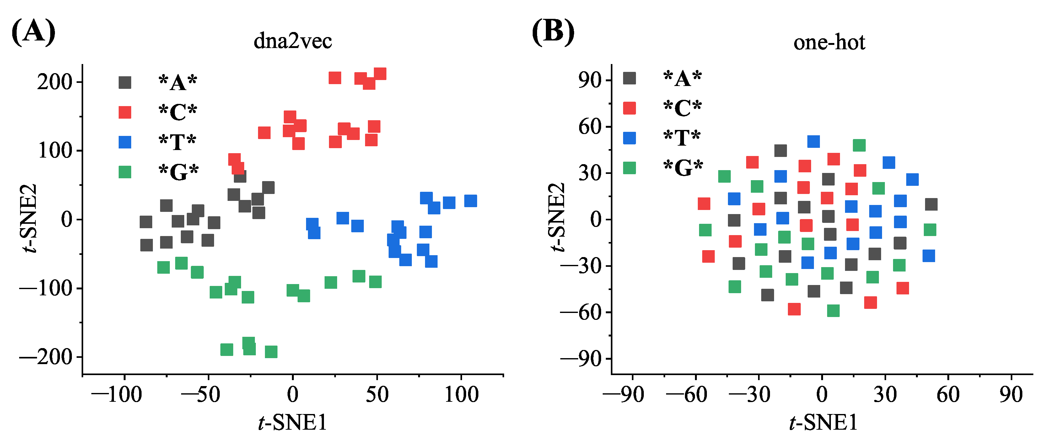In contrast to the dna2vec method, the one-hot encoding method cannot infer the connections between k-mer words for deeper association mining. The data visualization tool t-SNE was used to cluster the word vectors obtained by different encoding methods. Figure 4 shows the clustering effect of the three-mer word vectors based on dna2vec and one-hot encoding, and different three-mer vectors according to the nucleotide species at the central position are plotted. In the figure, the dna2vec-based encoding method better clustered similar word vectors, and their local clusters were clustered into larger clustering groups based on the same central nucleotides.

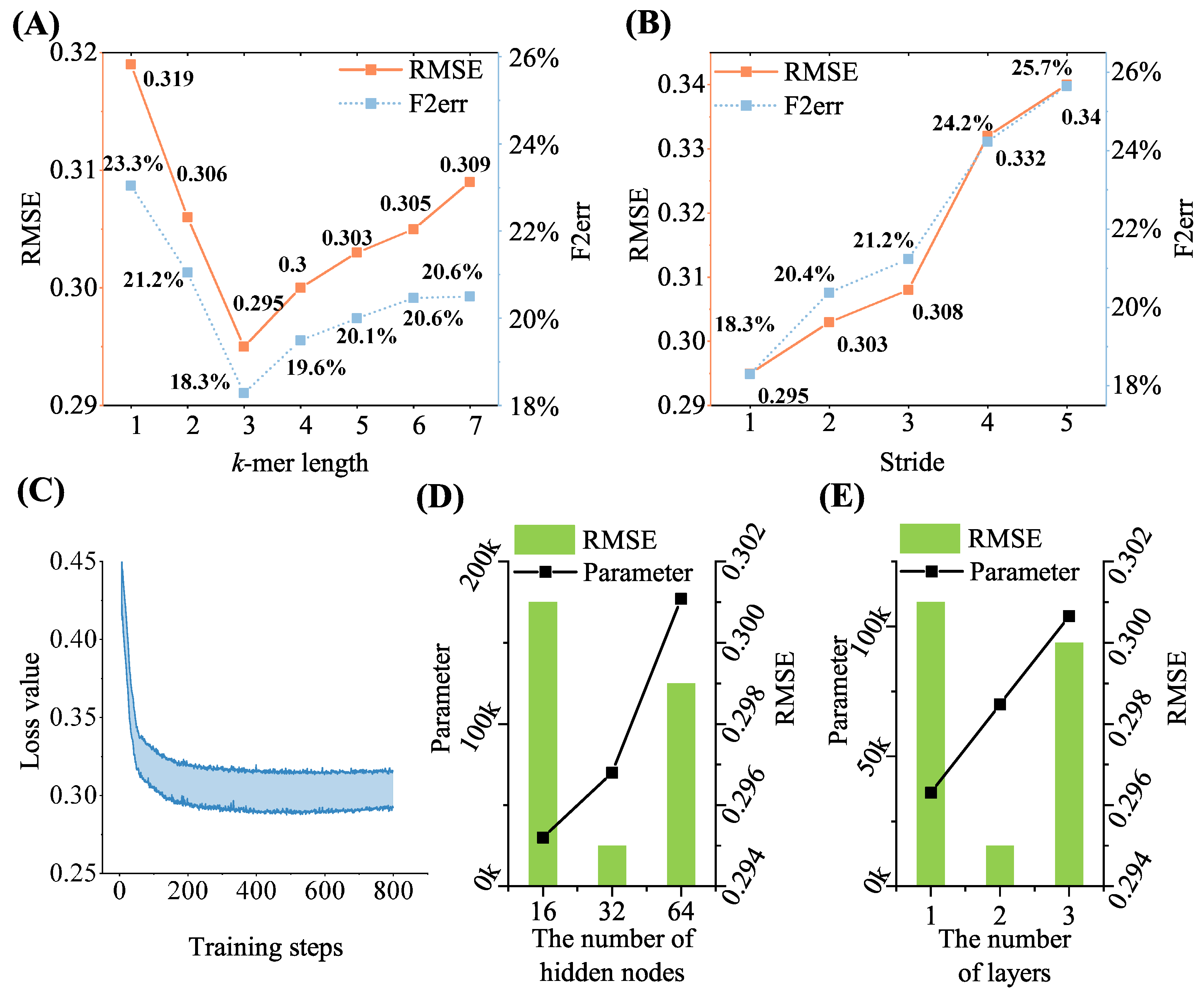
3.2. Parameter Optimization

The model parameters were trained using a 20-fold cross-validation method to comprehensively assess the proposed model. The dataset was divided into 20 folds, with 19 folds serving as the training set and 1 fold serving as the prediction set. This process was repeated 20 times, and the results were aggregated after 20 rounds of cross-validated predictions to obtain the prediction accuracy of our network.

To acquire the best-distributed representation of the sequences, the performance of the proposed model was tested with different step size (s) and k values. As depicted in Figure 5A, the performance of the model was the best when k was 3. This result can be attributed to the fact that in biology, an amino acid comprises three bases, and the process of segmenting a sequence into word vectors with $k=3$ shares a similar characteristic with this phenomenon. Then, k was set to 3, and the effect of different values of s on performance was tested. As Figure 5B indicates, the model’s performance deteriorated as the step size increased. Longer step lengths could lead to a loss of sequence information. This might result in a degradation of prediction performance. Therefore, the values of k and s were set to 3 and 1, respectively, during the following experiments on model performance calculation. On an Intel(R) Xeon Gold 5220R CPU with a maximum frequency of 2.2 GHz, the CPU times required to generate sequence representation using DLM and the proposed model were compared. Based on the SNP dataset, the process of generating three-mer sequence representation took only 4 min of CPU time, significantly reducing the transformation processing time from sequence to distributed representation compared to the DLM (334 min of CPU time).

The proposed model was completed with the PyTorch framework on an NVIDIA A6000 GPU server [33]. The model was trained with a batch size of 2560, and the initial learning rate was set to 0.0001. During the training process, RMSE was utilized to calculate the loss value between the predicted results and actual labels, and the adaptive moment estimation (Adam) algorithm was used to optimize the gradient descent [34]. The training process of this model is illustrated in Figure 5C. By observing the change in the loss value with the number of iterations, it was found that the loss value of the validation set started to increase at 450 rounds or more, indicating that the overfitting phenomenon had started to occur; therefore, the number of iterations was set to 450. Figure 5D,E illustrates the process of setting the number of hidden nodes and layers in a Bi-LSTM network, and the two-layer Bi-LSTM network with 32 hidden nodes is the optimal model. Setting more hidden nodes and deeper layers in the Bi-LSTM could lead to overfitting of the model, while a one-layer network or a smaller number of hidden nodes could lead to a lack of information acquisition. Compared to the four three-layer GRU networks with 128 hidden nodes used in the DLM, the number of parameters was reduced in the proposed sequencing depth prediction model because the sequence representation obtained through the k-mer and dna2vec in the sequence-encoding module contained more sequence information.

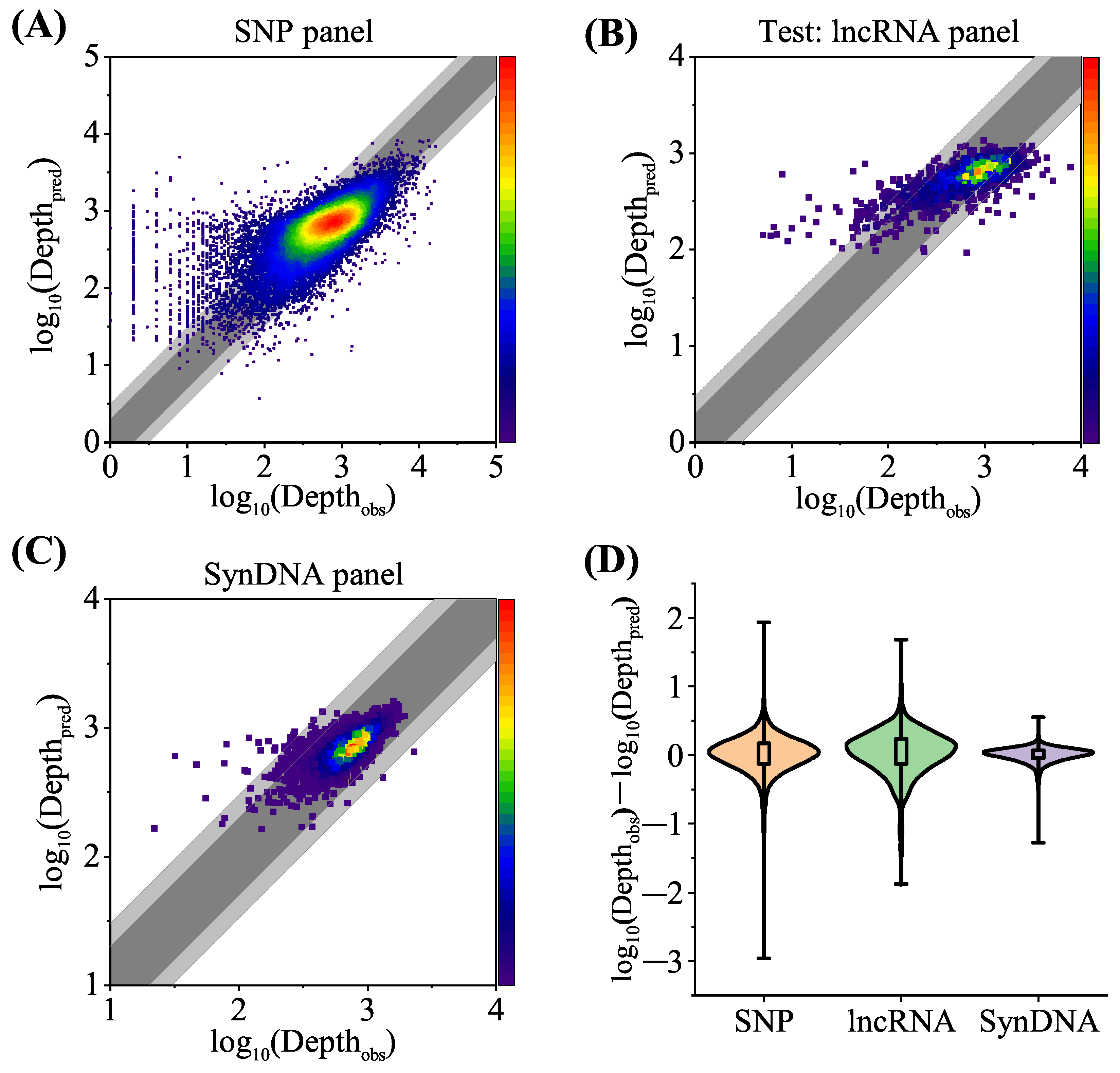
3.3. Predicted Results

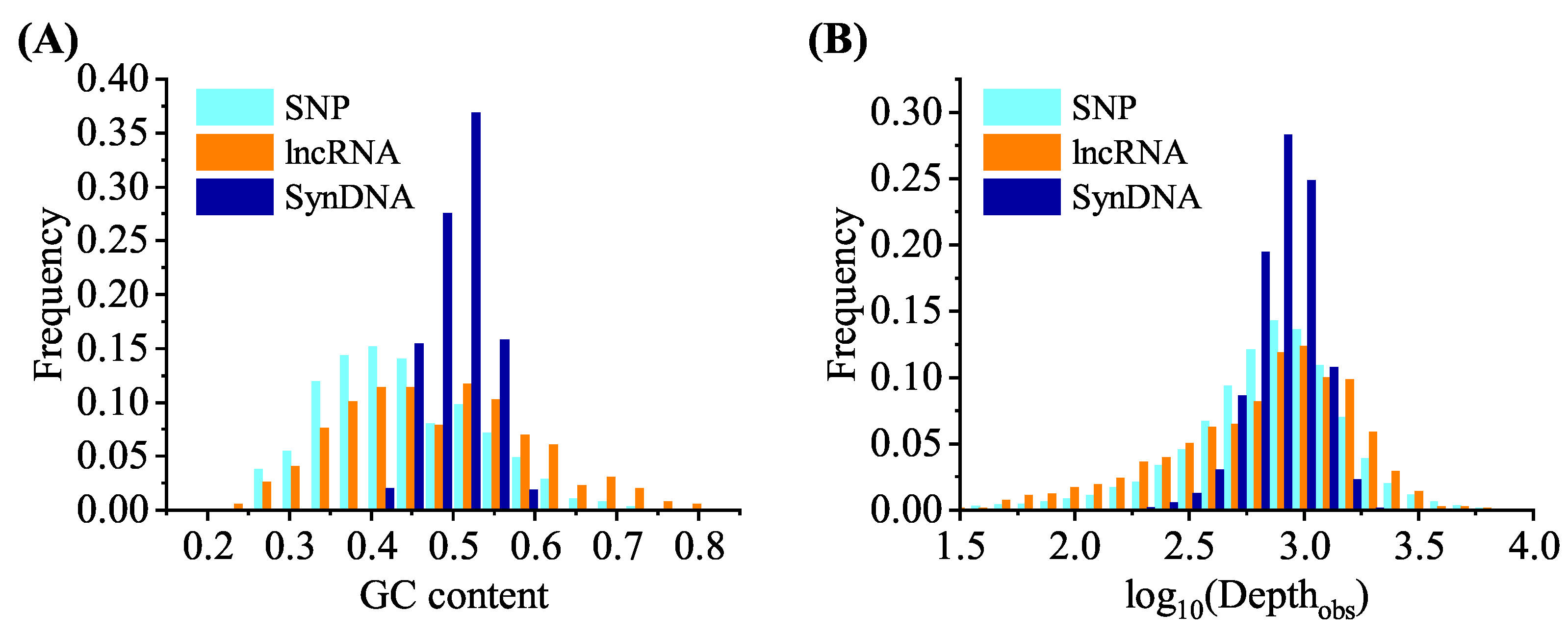
Figure 6A–C depict a comparison of the predicted and observed sequencing depth for the different datasets. The dark gray shading marks areas where the difference between the predicted sequencing depth and observed actual read depth was within a multiple of two, and the light gray indicates where the difference was within a multiple of three. Figure 6A shows the combined results of the SNP dataset after 20-fold cross validation. At a sequencing depth of 100 and above (i.e., ${log}_{10}($Depth${}_{obs})>2)$, the points combining predicted and observed depth were densely distributed in the gray area. Sequences with a lower observed sequencing depth in the SNP dataset had a ${log}_{10}($Depth${}_{pred}$) of between 1 and 3.5, while the majority of these probes had a lower GC content (average GC content of 0.31 for sequencing depth less than 100 and 0.45 for sequences depth greater than 100). An explanation for this phenomenon is that probes with a lower observed sequencing depth (such as a lower GC content) were more affected by random fluctuations in the experimental procedure, which could also affect the sequencing depth [9]. This also illustrates the importance of using GC content as an input to the dense module in the neural network.

To prove the effectiveness of the model in practical application scenarios, such as using the existing model to optimize the new probe design, the lncRNA dataset was taken as a prediction set from the SNP dataset, and the read depth of lncRNA was predicted through the model trained on the SNP dataset. It should be noted that although the lncRNA dataset and the SNP dataset had similar library preparation methods in terms of experimental work flow, hybridization temperature, and other relevant aspects, they differed in terms of the experimental operator, instrumentation, and reagents. In this study, the model obtained from a single fold of the 20-fold cross-validation process on the SNP dataset was employed to directly predict the probe log sequencing depth for the lncRNA dataset. Figure 6B displays the results of the lncRNA dataset generated from the proposed model trained on the SNP dataset. The proportion of points within the light gray region was marginally lower in the lncRNA compared to the SNP, and this decline might have been caused by the experimental changes associated with library preparation methods and other factors. However, because the proposed model only used the model trained in one fold of the SNP training process to predict the lncRNA log sequencing depth, this significantly reduced the cost of the sequencing probe design and prediction. The results of the lncRNA dataset show that the proposed model can predict the sequencing depth of probes obtained by similar library preparation methods to enable the generalization of method availability.

Figure 6C shows the SynDNA dataset prediction results of probes applied in DNA information storage. The points in the figure are mostly concentrated within the gray area. The generation of these sequences by the program led to a reduction in the probability of high or low GC content, hairpin structures, and homopolymers, which resulted in a more focused distribution of sequencing depth and enhanced prediction performance. Figure 6D shows the deviation between the predicted and observed log sequencing depth in different datasets. On each box whisker plot, the bottom of the box represents the 75th percentile, the top edge represents the 25th percentile, and the whisker length refers to the maximum and minimum values of the difference between the observed and predicted depths.

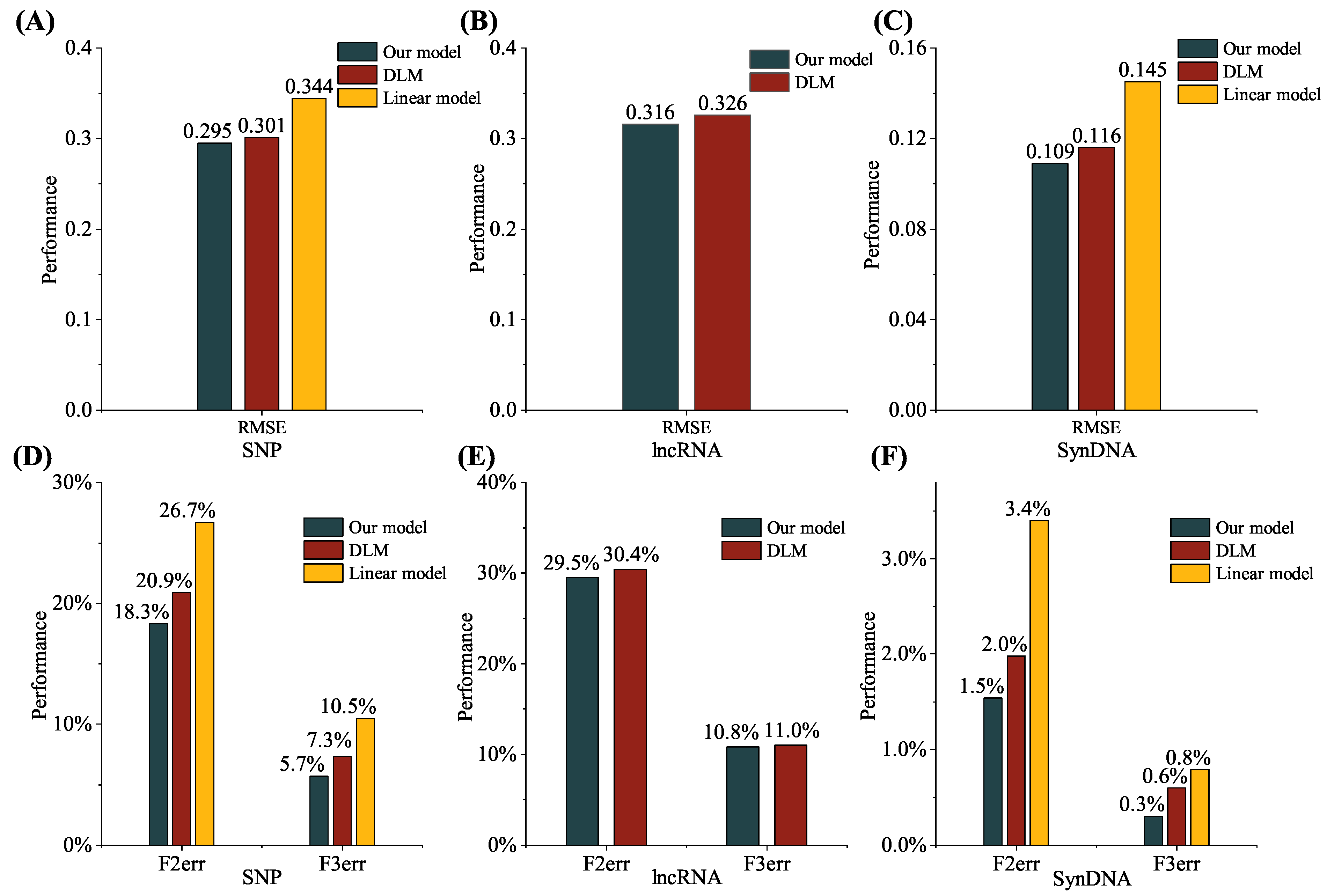
3.4. Performance Comparison with Other Methods

To better evaluate the performance of our model, Figure 7 demonstrates a performance comparison of different networks on three different datasets. F2err and F3err were applied to determine the proportion of sequences for which the error between the predicted and observed sequencing depth exceeded twofold and threefold, respectively, where RMSE represents the root mean square error across the dataset. The DLM and the linear model were employed for comparison with the proposed model. The DLM used the GRU network were used to process the target and probe sequences for sequencing depth prediction. The linear model used four biochemical features calculated by Nupack as input to predict the sequencing depth. The sequencing depth prediction performance for all competing methods was obtained from their respective papers.

As demonstrated in Figure 7, our model outperformed the DLM and the linear model in terms of RMSE, F2err, and F3err metrics on both the SNP and SynDNA datasets (F2err of 18.3%, F3err of 5.7%, and RMSE of 0.295 on the SNP dataset and F2err of 1.5%, F3err of 0.3%, and RMSE of 0.109 on the SynDNA dataset), indicating that better predictions were achieved for different types of probes. Our model also performed slightly better than DLM in predicting the sequencing depth of the lncRNA dataset using a onefold model trained on the SNP dataset (F2err of 29.5%, F3err of 10.8%, and RMSE of 0.316 on the lncRNA dataset). This suggests that it could achieve a better prediction performance for probes that use similar library preparation methods to predict their sequencing depth. The performance improvement can be attributed to the distributed representation of the sequence, as well as the utilization of Bi-LSTM and attention modules, to capture the long-range and short-range interactions in the sequences.

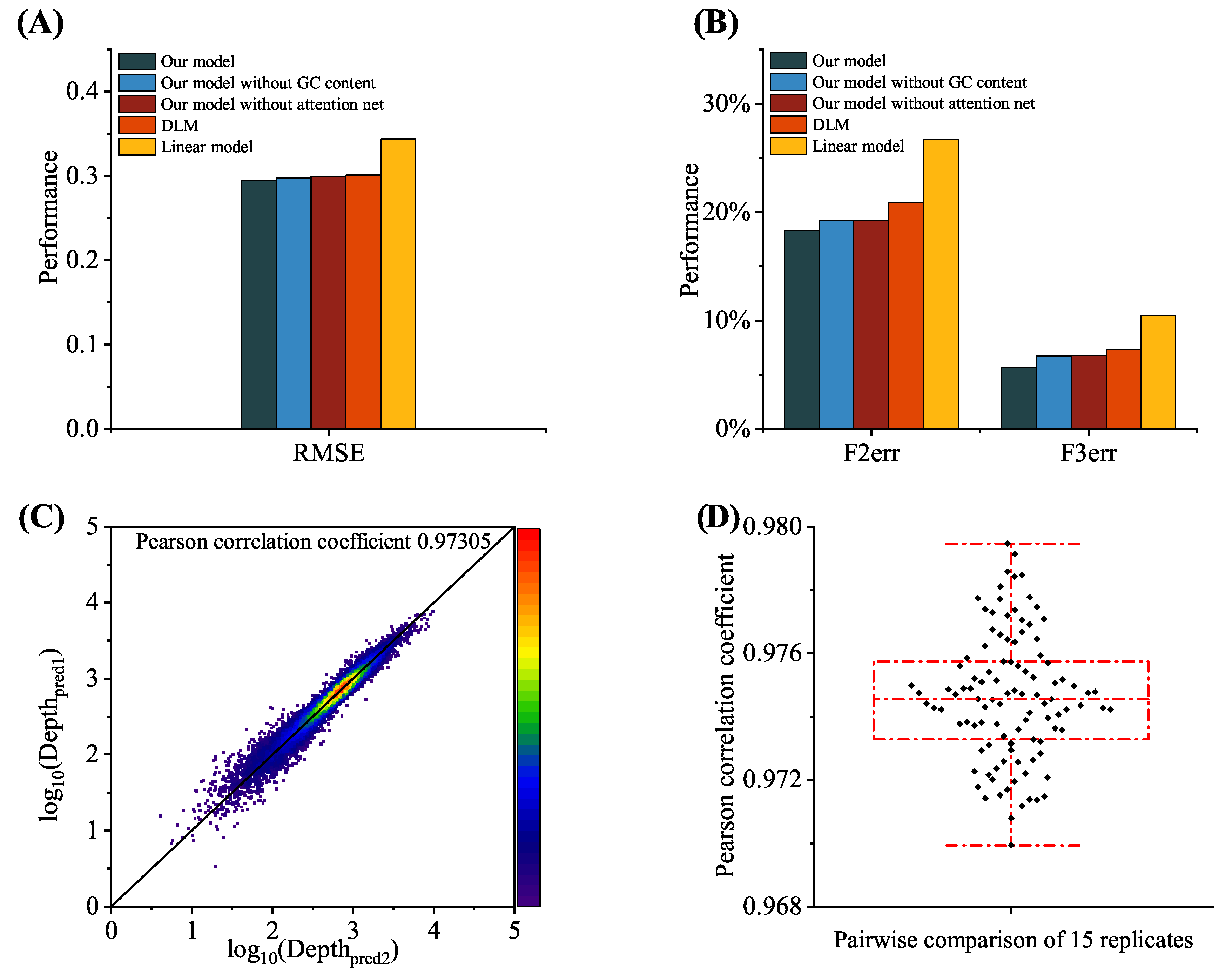
3.5. Ablation Experiments and Reliability Analysis

To verify the design superiority of the proposed model, two simplified models were compared with the proposed model using ablation experiments: our model (no GC feature) and our model (no attention). Figure 8A,B and

Table 1. Comparison of the performance of different neural networks and the number of parameters based on the SNP dataset.

	Parameter	Memory	Batch Size	RMSE
DLM	300 k	2369 MB	999	0.301
Our model	70 k	4055 MB	2560	0.295
Our model (no GC feature)	70 k	4027 MB	2560	0.298
Our model (no attention)	68 k	3953 MB	2560	0.299

present the performance results on the SNP dataset. Further analysis showed that the use of different modules resulted in different performance improvements. The GC content increased the amount of input information for the existing model and was related to the sequencing depth. The attention mechanism extracted the effect of different regions of the input sequence on the sequencing depth. Based on performance comparisons, the model using the attention mechanism with GC content achieved the best prediction performance.

As shown in Table 1, there are 70 k trainable parameters in the proposed sequencing depth prediction model, which is significantly less than the DLM (300 k in total), with the reduction in parameters mainly stemming from optimization of the number of hidden nodes and the number of network layers in the RNN module. The reduction in the number of parameters did not have a negative impact on prediction accuracy. Experiments conducted on publicly available data illustrate that the proposed model outperformed the DLM, as described in Figure 7. However, due to the large number of model parameters, to verify the robustness of the model and avoid overfitting phenomena or non-reproducibility being caused by too many parameters, several rounds of independent experiments were set up, verifying that the prediction results were highly consistent. The proposed model training process was repeated 15 times on the SNP dataset. Each round of training started with random parameters and stopped after 450 rounds. Figure 8C shows the comparison results of the log sequencing depth predictions from two independent prediction rounds. As presented in Figure 8D, Pearson’s r values for all 105 pairwise comparisons exceeded 0.970, which demonstrates that despite the difference in parameter initialization across independent experiments, the proposed model still generated relatively consistent prediction results.

4. Discussion and Conclusions

Targeted high-throughput sequencing of DNA has emerged as a superior technique in biomedical research. Although the cost of NGS has decreased exponentially over the years, the problem of poor sequencing uniformity remains a significant issue. Inefficient sequencing of high-depth targets and insufficient coverage of low-depth targets can result in a wasteful use of reads. Therefore, a low-complexity targeted sequencing depth prediction model was proposed in this paper to provide guidance for probe sequence analysis work. In this study, we implemented the prediction function of sequencing depth prediction using probe sequences. Our innovation can be summarized as follows. (1) A distributed representation of k-mer was trained using the word-embedding model, and a sequence-encoding model was constructed to realize the representation process from sequences to feature matrices. (2) The sequencing depth prediction model based on Bi-LSTM with ab attention mechanism was proposed to realize the sequencing depth prediction result of generating sequences from the feature matrix representation of probe sequences. Our model used a new sequence-encoding process that only took 4 min of CPU time for the SNP dataset. Compared with the complex biochemical calculations in DLM, our process was more efficient and convenient. The network architecture was optimized, and the parameters were reduced from 300 k to 70 k, which reduced the risk of overfitting. The prediction accuracy was improved based on the different datasets compared with the linear model and the DLM. The proposed model predicted the difference between predicted and observed sequencing depths with an F3err of 5.7% for SNP and 0.3% for SynDNA.

In conclusion, our model provides a practical solution for prediction of the sequencing depth of the probe sequence. In future work, the proposed model can be transferred and extended to other bioinformatics tasks. For example, the proposed model can be extended by constructing corresponding datasets and combining other types of features. The intermolecular interactions that occur between a large number of sequences in solution during target capture are modeled and analyzed to assess their impact on sequencing depth. Meanwhile, we can attempt to introduce a transformer [35] to optimize the existing sequencing depth prediction model to address the potential vanishing gradient problem of existing RNN models when sequentially processing long sequence information.

References

1. Jones, M.R.; Good, J.M. Targeted capture in evolutionary and ecological genomics. Mol. Ecol. 2016, 25, 185–202. [Google Scholar] [CrossRef] [PubMed] [Green Version]
2. Zhong, Y.; Xu, F.; Wu, J.; Schubert, J.; Li, M.M. Application of next generation sequencing in laboratory medicine. Ann. Lab. Med. 2021, 41, 25–43. [Google Scholar] [CrossRef] [PubMed]
3. Chen, W.; Wang, L.; Han, M.; Han, C.; Li, B. Sequencing barcode construction and identification methods based on block error-correction codes. Sci. China Life Sci. 2020, 63, 1580–1592. [Google Scholar] [CrossRef] [PubMed]
4. Chen, W.; Han, M.; Zhou, J.; Ge, Q.; Wang, P.; Zhang, X.; Zhu, S.; Song, L.; Yuan, Y. An artificial chromosome for data storage. Natl. Sci. Rev. 2021, 10, 361. [Google Scholar] [CrossRef]
5. Singh, R.R. Target enrichment approaches for next-generation sequencing applications in oncology. Diagnostics 2022, 12, 1539. [Google Scholar] [CrossRef]
6. Mertes, F.; ElSharawy, A.; Sauer, S.; van Helvoort, J.M.L.M.; van der Zaag, P.J.; Franke, A.; Nilsson, M.; Lehrach, H.; Brookes, A.J. Targeted enrichment of genomic DNA regions for next-generation sequencing. Brief. Funct. Genom. 2011, 10, 374–486. [Google Scholar] [CrossRef]
7. Mamanova, L.; Coffey, A.J.; Scott, C.E.; Kozarewa, I.; Turner, E.H.; Kumar, A.; Howard, E.; Shendure, J.; Turner, D.J. Target-enrichment strategies for next-generation sequencing. Nat. Methods 2010, 7, 111–118. [Google Scholar] [CrossRef]
8. Gnirke, A.; Melnikov, A.; Maguire, J.; Rogov, P.; LeProust, E.; Brockman, W.; Fennell, T.; Giannoukos, G.; Fisher, S.; Russ, C.; et al. Solution hybrid selection with ultra-long oligonucleotides for massively parallel targeted sequencing. Nat. Biotechnol. 2009, 27, 182–189. [Google Scholar] [CrossRef] [Green Version]
9. Zhang, J.X.; Yordanov, B.; Gaunt, A.; Wang, M.X.; Dai, P.; Chen, Y.J.; Zhang, K.; Fang, J.Z.; Dalchau, N.; Li, J.M.; et al. A deep learning model for predicting next-generation sequencing depth from DNA sequence. Nat. Commun. 2021, 12, 4387. [Google Scholar] [CrossRef]
10. Redmon, J.; Divvala, S.; Girshick, R.; Farhadi, A. You only look once: Unified, real-time object detection. In Proceedings of the IEEE Conference on Computer Vision and Pattern Recognition (CVPR), Las Vegas, NV, USA, 27–30 June 2016; pp. 779–788. [Google Scholar]
11. Otter, D.W.; Medina, J.R.; Kalita, J.K. A survey of the usages of deep learning for natural language processing. IEEE Trans. Neural Netw. Learn. Syst. 2021, 32, 604–624. [Google Scholar] [CrossRef] [Green Version]
12. Chen, W.; Chen, W.; Song, L. Enhancing deep multimedia recommendations using graph embeddings. In Proceedings of the IEEE Conference on Multimedia Information Processing and Retrieval (MIPR), Shenzhen, China, 6–8 August 2020; pp. 161–166. [Google Scholar]
13. Srinivasan, S.S.; Gong, Y.; Xu, S.; Hwang, A.; Xu, M.; Girgenti, M.J.; Zhang, J. InsuLock: A weakly supervised learning approach for accurate insulator prediction, and variant impact quantification. Genes 2022, 13, 621. [Google Scholar] [CrossRef] [PubMed]
14. Cohen, J.D.; Li, L.; Wang, Y.X.; Thoburn, C.; Afsari, B.; Danilova, L.; Douville, C.; Javed, A.A.; Wong, F.; Mattox, A.; et al. Detection and localization of surgically resectable cancers with a multi-analyte blood test. Science 2018, 359, 926–930. [Google Scholar] [CrossRef] [Green Version]
15. Angenent-Mari, N.M.; Garruss, A.S.; Soenksen, L.R.; Church, G.; Collins, J.J. A deep learning approach to programmable RNA switches. Nat. Commun. 2020, 11, 5057. [Google Scholar] [CrossRef] [PubMed]
16. Chen, W.; Zhang, P.; Song, L.; Yang, J.; Han, C. Simulation of nanopore sequencing signals based on BiGRU. Sensors 2020, 20, 7244. [Google Scholar] [CrossRef] [PubMed]
17. Berrar, D.; Dubitzky, W. Deep learning in bioinformatics and biomedicine. Brief. Bioinform. 2021, 22, 1513–1514. [Google Scholar] [CrossRef]
18. Zadeh, J.N.; Steenberg, C.D.; Bois, J.S.; Wolfe, B.R.; Pierce, M.B.; Khan, A.R.; Dirks, R.M.; Pierce, N.A. NUPACK: Analysis and design of nucleic acid systems. J. Comput. Chem. 2008, 32, 170–173. [Google Scholar] [CrossRef]
19. Ng, P. dna2vec: Consistent vector representations of variable-length k-mers. arXiv 2017, arXiv:1701.06279. [Google Scholar]
20. Ceze, L.; Nivala, J.; Strauss, K. Molecular digital data storage using DNA. Nat. Rev. Genet. 2019, 20, 456–466. [Google Scholar] [CrossRef]
21. Li, H.; Durbin, R. Fast and accurate short read alignment with Burrows-Wheeler transform. Bioinformatics 2009, 25, 1754–1760. [Google Scholar] [CrossRef] [Green Version]
22. Benjamini, Y.; Speed, T.P. Summarizing and correcting the GC content bias in high-throughput sequencing. Nucleic Acids Res. 2012, 10, e72. [Google Scholar] [CrossRef] [Green Version]
23. Browne, P.D.; Nielsen, T.K.; Kot, W.; Aggerholm, A.; Gilbert, M.T.P.; Puetz, L.; Rasmussen, M.; Zervas, A.; Hansen, L.H. GC bias affects genomic and metagenomic reconstructions, underrepresenting GC-poor organisms. Gigascience 2020, 9, giaa008. [Google Scholar] [CrossRef]
24. Mikolov, T.; Chen, K.; Corrado, G.; Dean, J. Efficient estimation of word representations in vector space. arXiv 2013, arXiv:1301.3781. [Google Scholar]
25. Deng, C.; Lai, G.; Deng, H. Improving word vector model with part-of-speech and dependency grammar information. CAAI Trans. Intell. Technol. 2020, 5, 276–282. [Google Scholar] [CrossRef]
26. Yu, Y.; Si, X.; Hu, C.; Zhang, J. A review of recurrent neural networks: LSTM cells and network architectures. Neural Comput. 2019, 31, 1235–1270. [Google Scholar] [CrossRef]
27. He, B.; Wu, H.; Li, C.; Song, L.; Chen, W. K-CSRL: Knowledge enhanced conversational semantic role labeling. In Proceedings of the 2021 13th International Conference on Machine Learning and Computing (ICMLC 2021), Shenzhen, China, 26 February–1 March 2021; pp. 530–555. [Google Scholar]
28. Basiri, M.E.; Nemati, S.; Abdar, M.; Cambria, E.; Acharya, U.R. ABCDM: An attention-based bidirectional CNN-RNN deep model for sentiment analysis. Future Gener. Comput. Syst. 2021, 115, 279–294. [Google Scholar] [CrossRef]
29. Niu, Z.; Zhong, G.; Yu, H. A review on the attention mechanism of deep learning. Neurocomputing 2021, 452, 48–62. [Google Scholar] [CrossRef]
30. Chaudhari, S.; Mithal, V.; Polatkan, G.; Ramanath, R. An attentive survey of attention models. ACM Trans. Intell. Syst. Technol. 2021, 53, 1–32. [Google Scholar] [CrossRef]
31. Srivastava, N.; Hinton, G.; Krizhevsky, A.; Sutskever, I.; Salakhutdinov, R. Dropout: A simple way to prevent neural networks from overfitting. J. Mach. Learn. Res. 2014, 15, 1929–1958. [Google Scholar]
32. Lv, Z.; Ding, H.; Wang, L.; Zou, Q. A convolutional neural network using dinucleotide one-hot encoder for identifying DNA n6-methyladenine sites in the rice genome. Neurocomputing 2021, 422, 214–221. [Google Scholar] [CrossRef]
33. Paszke, A.; Gross, S.; Massa, F.; Lerer, A.; Bradbury, J.; Chanan, G.; Killeen, T.; Lin, Z.; Gimelshein, N.; Antiga, L.; et al. PyTorch: An imperative style, high-performance deep learning library. Adv. Neural Inf. Process. Syst. 2019, 32. [Google Scholar]
34. Kingma, D.; Ba, J. Adam: A method for stochastic optimization. arXiv 2014, arXiv:1412.6980. [Google Scholar]
35. Ji, Y.; Zhou, Z.; Liu, H.; Davuluri, R. DNABERT: Pre-trained Bidirectional Encoder Representations from Transformers model for DNA-language in genome. Bioinformatics 2021, 37, 2112–2120. [Google Scholar] [CrossRef] [PubMed]
Figure 1. Overview of targeted sequencing methods and different sequencing depth prediction models. (A) The specific process of targeted sequencing includes probe sequence design, sample library construction, probe and sample library hybridization capture, elution, and sequencing. (B) The proposed model is compared with the existing sequencing depth prediction model, DLM, and the proposed model differs from the sequence encoding model and the sequencing depth prediction model.
Applsci 13 06996 g001
Figure 2. Histograms of the frequency distribution of GC content and log sequencing depth for the three datasets. (A) Frequency distribution histograms of GC content for the SNP, lncRNA, and SynDNA datasets. (B) Histogram of the frequency distribution of the log sequencing depth for the three probe datasets.
Applsci 13 06996 g002
Figure 3. Schematic representation of the sequence-encoding phase and the sequencing depth prediction phase of the proposed model. (A) A flow chart demonstrating the proposed model for generating sequencing depth prediction results from probe sequences. The light gray area represents the sequence-encoding model, and the light yellow area represents the sequencing depth prediction model. (B) Overview of converting sequences into a feature matrix via k-mer and dna2vec processing. (C) Overview of the process of using the feature matrices of probe and target sequences to generate the log sequencing depth prediction result.
Applsci 13 06996 g003
Figure 4. Visualization of features extracted by dna2vec and one-hot for three-mer word vectors using t-SNE. (A) The word vector clustering result for three-mer encoding by dna2vec. The different colors represent the different nucleotide species in the central position, where “*” represents nucleotide. (B) The clustering result of word vector encoding by one-hot for three-mer encoding.
Applsci 13 06996 g004
Figure 5. Optimization of different network architecture parameters. (A) Comparison of the proposed model with different k-mer lengths on the SNP dataset under the RMSE and F2err, where F2err represents the proportion of predicted sequencing depth and observed sequencing depth errors exceeding twofold, and RMSE represents the root mean square error across the dataset. (B) Comparison of RMSE and F2err results for different step sizes on the SNP dataset with a length of 3 mer. (C) The plot of loss values versus training iteration steps shows the variation of loss values with training rounds for each fold of the proposed model in the 20-fold cross-validation run. The area between the two lines indicates the range of loss values over the 20 training rounds. (D) Comparison of RMSE and parameters for different hidden nodes in two-layer Bi-LSTM on the SNP dataset. (E) Comparison of RMSE and parameters for different layers of a Bi-LSTM with 32 hidden nodes on the SNP dataset.
Applsci 13 06996 g005
Figure 6. Results of 20-fold cross-validation training of the proposed model based on different datasets. (AC) Comparison of predicted log sequencing depth with observed log sequencing depth for different datasets, where (AC) are under the SNP dataset, lncRNA dataset, and SynDNA dataset, respectively. These plots are a summary of the sequencing depth prediction results for all validation sets in the 20-fold cross-validation training. (D) The deviation of sequencing depth between predicted and observed depth for different datasets.
Applsci 13 06996 g006
Figure 7. Performance comparison of our model and the competing models on different datasets. (A,D) Comparison of our model with DLM and the linear model on the SNP dataset under the F2err, F3err, and RMSE. (B,E) Comparison of our model with DLM on the lncRNA dataset under the F2err, F3err, and RMSE. (C,F) Comparison of our model with DLM and the linear model on the SynDNA dataset under the F2err, F3err, and RMSE.
Applsci 13 06996 g007
Figure 8. Results of the robustness analysis of the proposed model and ablation experiments based on the SNP dataset. (A) Performance comparison of our model, our model (no GC feature), our model (no attention), DLM, and the linear model on the SNP dataset under the RMSE. (B) Performance comparison of different models on the SNP dataset under the F2err and F3err. (C) Comparison of sequencing depth predictions from two independent prediction rounds. (D) Summary of 105 pairwise comparative correlation coefficients for the results of 15 training process runs.
Applsci 13 06996 g008