Systematic Review

PREFMoDeL: A Systematic Review and Proposed Taxonomy of Biomolecular Features for Deep Learning

1
Department of Biochemistry, University of Washington, Seattle, WA 98195, USA
2
Institute for Protein Design, University of Washington, Seattle, WA 98195, USA
3
Graduate Program in Biological Physics, Structure and Design, University of Washington, Seattle, WA 98195, USA
4
Department of Biochemistry and Biophysics, Oregon State University, Corvallis, OR 97331-7305, USA
*
Author to whom correspondence should be addressed.
Appl. Sci. 2023, 13(7), 4356; https://doi.org/10.3390/app13074356
Submission received: 5 February 2023 / Revised: 8 March 2023 / Accepted: 9 March 2023 / Published: 29 March 2023
(This article belongs to the Special Issue Machine Learning in Bioinformatics: Latest Advances and Prospects)

Abstract

:
Of fundamental importance in biochemical and biomedical research is understanding a molecule’s biological properties—its structure, its function(s), and its activity(ies). To this end, computational methods in Artificial Intelligence, in particular Deep Learning (DL), have been applied to further biomolecular understanding—from analysis and prediction of protein–protein and protein–ligand interactions to drug discovery and design. While choosing the most appropriate DL architecture is vitally important to accurately model the task at hand, equally important is choosing the features used as input to represent molecular properties in these DL models. Through hypothesis testing, bioinformaticians have created thousands of engineered features for biomolecules such as proteins and their ligands. Herein we present an organizational taxonomy for biomolecular features extracted from 808 articles from across the scientific literature. This objective view of biomolecular features can reduce various forms of experimental and/or investigator bias and additionally facilitate feature selection in biomolecular analysis and design tasks. The resulting dataset contains 1360 nondeduplicated features, and a sample of these features were classified by their properties, clustered, and used to suggest new features. The complete feature dataset (the Public Repository of Engineered Features for Molecular Deep Learning, PREFMoDeL) is released for collaborative sourcing on the web.

Graphical Abstract

1. Introduction

Modern experimental advances have enabled scientists to analyze molecular properties, and to design completely new molecules with beneficial functions [1,2,3,4]. For example, the antibiotic penicillin was first discovered as a natural product in the mold Penicillium rubens, but subsequent drug design produced the stronger, faster-acting, and broader-spectrum antibiotic amoxicillin [5]. Furthermore, not limited to only small molecules, protein design for therapeutic applications has recently grown by leaps and bounds with the introduction of deep neural networks for structure prediction [6,7] and sequence design [8]. SkyCovione [9], the first computationally designed nanoparticle vaccine developed for COVID-19, elicits a superior immune response than existing mRNA vaccines, and has been approved for use in South Korea to fight COVID-19. Drugs such as amoxicillin and SkyCovione could not save lives today were it not for careful characterization of experimental data.
From large datasets, analytical measurements (“observables”) are refined into more concise “features”—specific subsets that capture relevant properties of the sample. For example, features describing amoxicillin might include its solubility, its bioavailability, the set of endogenous proteins it is known to bind to (so-called “promiscuous” drugs can bind to multiple receptors [10], see below), and the crystal structures of these bound complexes. Similarly, the SkyCovione nanoparticle may be described by its elicited antibody titer, its retention volume distribution by size-exclusion chromatography, or the kinetic association constant between its domains and the SARS-CoV-2 spike. These data are most often generated from various experimental assays and screening protocols, and reliable data gathering requires the skills necessary to prepare the sample and operate the instrument. Designing features based on the resulting data is often challenging as the high level of expertise required to accurately interpret the experimental results is often exclusive to the expertise required for feature design. Cursory instrument operation, incomplete knowledge of experimental protocols, and improper analysis can lead to erroneous features because each step can introduce a distinct form of error. These errors are discussed in Section 2.3.3.
Promiscuity refers to the behavior of a given ligand or receptor to bind to multiple receptors or ligands, respectively, each with a high affinity (distinguished by whether the kinetic dissociation constant of the protein–ligand complex is less than 10 μ M ). Promiscuous drugs are usually small and hydrophobic (which reduces the required specificity of interaction imposed by binding site electrostatics and hydrogen bonding, while retaining interaction strength) and promiscuous binding sites are able to accommodate diverse ligands through complementary hydrophobicity and dynamics [11]. Promiscuity may be a desired function of a designed drug or protein in some applications, but it may also manifest as undesired side effects; therefore, the careful accounting of promiscuity effects is encouraged. Recent work has investigated the structure–function relationship of promiscuity [12,13,14], and a comprehensive toolkit to analyze and optimize promiscuity effects would be immensely helpful, but one has not, to our knowledge, been published.
Many experimental assays will yield nonuseful or redundant information for the study of interest, so scientists routinely judge whether the features they design and refine contribute meaningfully to analysis—indeed, this process is analogous to the scientific method itself (Figure 1). Often new features (as well as new hypotheses) are needed to model a biochemical phenotype, so they are developed through feature engineering. In the machine learning field where the choice of input data is important  [15], successful network training is inextricably linked to feature choice.
In the language of features, a hypothesis is a falsifiable statement about an outcome of a proposed experiment given sufficient enumerated premises and whose falsification is contingent on the interpretation of measured features. Hypotheses are closely related to features [16], although key differences exist. While hypotheses are conceptual and designed to directly connect a phenomenon to an experimental outcome, the meaning of a feature (often in equation form or as a function in a computer program) is less directly interpretable. Separability is yet another factor: features may contribute supporting or falsifying information towards one or more hypotheses just as scientific hypotheses may be written in a way that requires the measurement and analysis of one or more features. A feature (or features) may be well selected to reflect the encoded hypothesis (or hypotheses), or not. A well-written feature would be as close as possible to representing the encoding of a single hypothesis, and achieves the following parameters: it is both human- and computer-interpretable; there is a one-to-one relationship between the hypothesis written and the feature computed; and the feature directly addresses the hypothesis. In short, a feature should be a hypothesis, but in a computationally accessible form such as an equation or in a programming language.
The extent to which existing feature–hypothesis pairs satisfy these conditions has not, to our knowledge, been investigated in the literature in part because a comprehensive enumeration of all features in the literature has not been put forth and because multiple orthogonal features can be used to evaluate a given hypothesis. Because a single hypothesis is often supported by multiple features, features in the scientific literature are likely at least as numerous as scientific hypotheses.
For these reasons, a comprehensive analysis of all features reported in the literature is a nearly impossible task, but is nonetheless a valuable endeavor that may be achieved through an open-source community-based effort. To start this process, the focus of this work is to describe a systematic review and the resulting development of a taxonomy of an initial representative sample of engineered molecular features based on their properties (in this study, “properties” refers to qualities that distinguish between two or more distinct groups of features—in other words, properties are “meta-features”). As an example of how this feature database (the Public Repository of Engineered Features for Molecular Deep Learning, PREFMoDeL) can be used, we have analyzed—without the detailed knowledge of how specific feature selections impact performance in various deep learning tasks—correlations between feature properties and visualized feature space using t-distributed stochastic neighborhood embedding (t-SNE).
The source PREFMoDeL table is presented in a community-editable repository (https://github.com/picodase/PREFMoDeL, accessd on 19 February 2023) which gives researchers an overarching view of the state of the art of biomolecular feature engineering, and to determine whether certain features are potentially useful or not. Additionally, we encourage researchers to perform their own analyses (including using other methods apart from t-SNE), to assess the appropriateness of a given feature selection to their own specific deep learning task(s). An additional benefit of our presented analysis and taxonomy is that gaps and underrepresentation of feature types in the literature are easily noticeable and therefore, addressable. We provide several examples of underrepresented feature taxa in our discussion below.
While particular attention is paid to the properties of biomolecular features, many of these properties are universal as they can describe broader categories of molecules. Additionally, the set of enumerated properties constituting the taxonomy is logically extensible, and adding features that are specific to other classes of molecules is easily accomplished.

2. Background

2.1. Vocabulary

Before discussing molecular analysis and design, features, and feature engineering, it is helpful to define several key terms. This initial work is focused on the class of biological molecules (biomolecules), more specifically proteins and ligands. The word protein denotes an amino acid polymer whether structured, fibrous, or intrinsically disordered. The word ligand indicates a molecule from the enormous class of compounds that bind to proteins and thus modulate their function. Ligands can include small organic molecules, carbohydrates, lipids, nucleic acids, inorganic compounds, clathrates, and organometallic compounds. As biological activity can be described reductively as a prescribed set of protein–ligand interactions, our study has broad utility for biomolecular analysis and design.

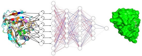
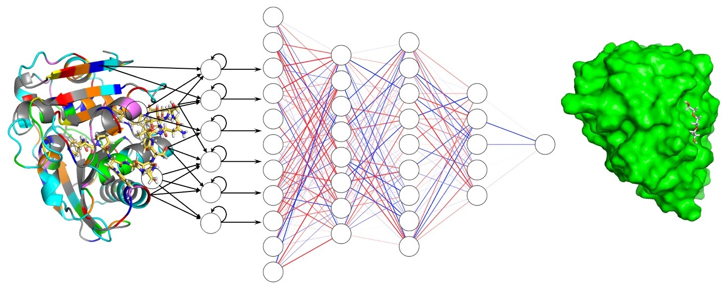
2.2. Parts of a Machine Learning Model

Features are used as input for a machine learning (ML) model to learn a transformation through parameter optimization. ML models learn the transformation F ( input ) = output by iteration over a training dataset. A ML model is composed of four parts: the model architecture, the loss function, the learned parameters mapping input to output, and the features.
The model architecture is the structure which defines how data are processed, where data often flow through multiple layers of composed functions. Architectures might vary from one another by the number of layers in a neural network, the number of nodes, layer dimensionality, layer arrangement, layer connectivity, and the model composition (modularity). Architectures tend to fall into two general classes based on the input data they can accept. A convolutional neural network (CNN) takes dimensional feature vectors—those that can be measured along an n-dimensional (ND) space—as input, and uses them to learn geometric information in that space based on locality [17]. Alternately, a graph neural network (GNN) operates on network features (or graphs)—those that can be represented as nodes connected by edges—so they learn topological information about input graphs [18]. Both of these networks are formed from layers that can be evaluated in a feed-forward manner (passed forward linearly from one layer to the next, e.g., from layer A B C ) or through a feedback manner (passed to a previous layer, e.g., taking a path from A B C A ). Note that the feedback architecture, which defines how features flow through the model, is distinct from the backpropagation algorithm, which updates the gradients of the model parameters between adjacent layers with respect to these features and is a common mechanism for all modern neural networks. These basic components may be composed in sequential layers and arranged to form more complex architectures such as autoencoders and transformers [19], and finally applied to biological problems [20,21].
The loss function is the part of the architecture which measures the “correctness” of model predictions [22,23]. It is typically composed of several terms that together teach the model to be “less incorrect” in specific, measurable ways through training. For example, a common loss function term for continuous features is the L2 norm or through-space distance. The categorical cross entropy (CCE) is a popular loss term for discrete features.
The parameters of the model are variables during training and are updated iteratively in order to minimize the loss function with respect to the architecture and features. After input features are passed through the layers of the network, the loss function is evaluated and used to compute the gradient of the loss with respect to each input. Backpropagation of these gradients [24,25] through the network informs the change in each parameter, with the guidance of an optimization algorithm [26] such as stochastic gradient descent (SGD). Over epochs of training, the parameters are fine-tuned to better compute F.
Lastly, features are as explained above: mathematical representations of relevant data. In other words, features are the evidence that the model observes to draw conclusions about the dataset using the hypothesis specified by the model structure. While all components of a neural network encode induced hypotheses about the system of study, the design of features that behave well in machine learning models, and of models that efficiently process input features, are active areas of discussion [27]. Features can be used to predict the target features of validation data sets that were not used for training the network (a task termed “supervised learning”, i.e., predicting a target feature f pred = F ( f input , 1 , . . . , f input , N ) ), to cluster the data and determine their underlying structure (“unsupervised learning”, i.e., calculating all pairwise relationships between feature f i and f j ), or to impute incomplete input feature columns and/or target features given other feature columns (“semi-supervised learning”, i.e., predicting features f pred , f missing , 1 , . . . f missing , M = F ( f input , 1 , . . . f input , N )). The choice of features is highly critical to successful modeling and frequently requires expert insight, and it will dictate the speed of learning, the speed of prediction, prediction accuracy, and the complexity of the function F.

2.3. Features and Feature Engineering as Analogues to the Scientific Method

A feature is a number or collection of numerical values that describes some direct or processed experimental observable. Any form of data can be converted into a feature if it can be assigned a numerical value. For example, the crystal structure of a protein consists of a set of datapoints (atoms) with several attributes: Cartesian position ( x , y , z ) , element (N, C, O, H), atom type (Calpha, C=O), B-factor, and more. Each of these attributes is a feature of that molecule and the experimental conditions under which the data were collected. At first glance, attributes such as element and atom type are categorical non-numeric values, but they can be converted into numbers using several strategies. These strategies might include using the isotopically averaged mass of the atom (14.007, 12.011, 15.999, and 1.008 au for each element, respectively) or using one-hot encoding (for example, 1000, 0100, 0010, 0001 for each element, respectively). While the strategy one chooses to encode their data is often subjective, algorithmically the results based on the encoding chosen is objective, and thus one must think carefully about how their data can best be represented.
Generic features can describe all types of objects, but only a subset of documented mathematical features have analogues in biomolecular representations. Furthermore, biomolecules have some features that other objects lack. For example, for an iris classification task, a certain flower might have the sepal length of 5.1 cm. Other objects, such as people, trees, or buildings, also have associated lengths. However, consider a particular protein–ligand pair that has the kinetic dissociation constant of K d = 0.14 millimolar (Figure 2). Flowers, people, trees, and buildings do not have well-defined notions of kinetic dissociation constants because they are not molecules and cannot be characterized in this manner.
However, just because a feature exists does not mean it is useful for a task of interest. Indeed, scientists routinely evaluate what the features they derive from their data suggest about the systems they study, which has led to the calculation of feature importance [28] and guidance for feature selection [29,30]. Often new features (like new hypotheses) are needed to explain a biochemical phenotype, so they are developed through feature engineering. In this process, features are equivalent to hypotheses of relevance.

2.3.1. The Importance of Feature Relevance

Features must be relevant to the problem they are being used to solve [29,30,31,32,33]: although the color of the iris (purple) would not help to distinguish between the three species in the iris training dataset, the length of the sepal can meaningfully provide this distinction. Furthermore, all relevant features must be represented at the time analysis or design decisions are made. However, these are challenging conditions to guarantee because it is impossible to measure the relevance of any feature before training a network. Instead, prior knowledge from past experiments is used to inform feature selection.

2.3.2. Desirable Feature Characteristics

Features that allow convenient, efficient, and stable network training (so-called “ideal features”) satisfy certain mathematical properties. To our knowledge, no biomolecular features satisfy all of them, and most satisfy fewer than half. Ideally, a given feature f must satisfy the following:
  • Representativeness: f accurately represents the underlying phenomenon.
  • Fixed dimension: f is of a fixed size, such as an appropriately shaped NumPy array.
  • Continuity: f takes continuous values.
  • Differentiability: f is differentiable.
  • Normalizability: f is normalized or normalizable to the interval (0,1) or the interval (−1,1).
  • Linearizability: If f is exponential or nonlinear, f can be linearized.
  • Reversibility: f is generated by a lossless transform T R that can be inverted, such that f = T R 1 T R f .
  • Example uniqueness: f is unique for a given input i. Similar to the concept of one-to-one in linear algebra.
  • SE(3) invariance or SE(3) equivariance: A rotation or translation in space either does not change (invariant) or evenly changes (equivariant) the values in f, respectively.
The significance and examples of applications of these ideal features are described in Supplementary Table S1. These mathematical properties are known for classifying features of all types of objects, but biomolecules have specific properties that other objects do not have. In order to evaluate these biomolecule-specific properties, a literature survey was conducted. Features were enumerated and classified according to a list of biomolecule-specific properties which was developed during the investigation. The collection and analysis process and the properties of this dataset are described in detail below.

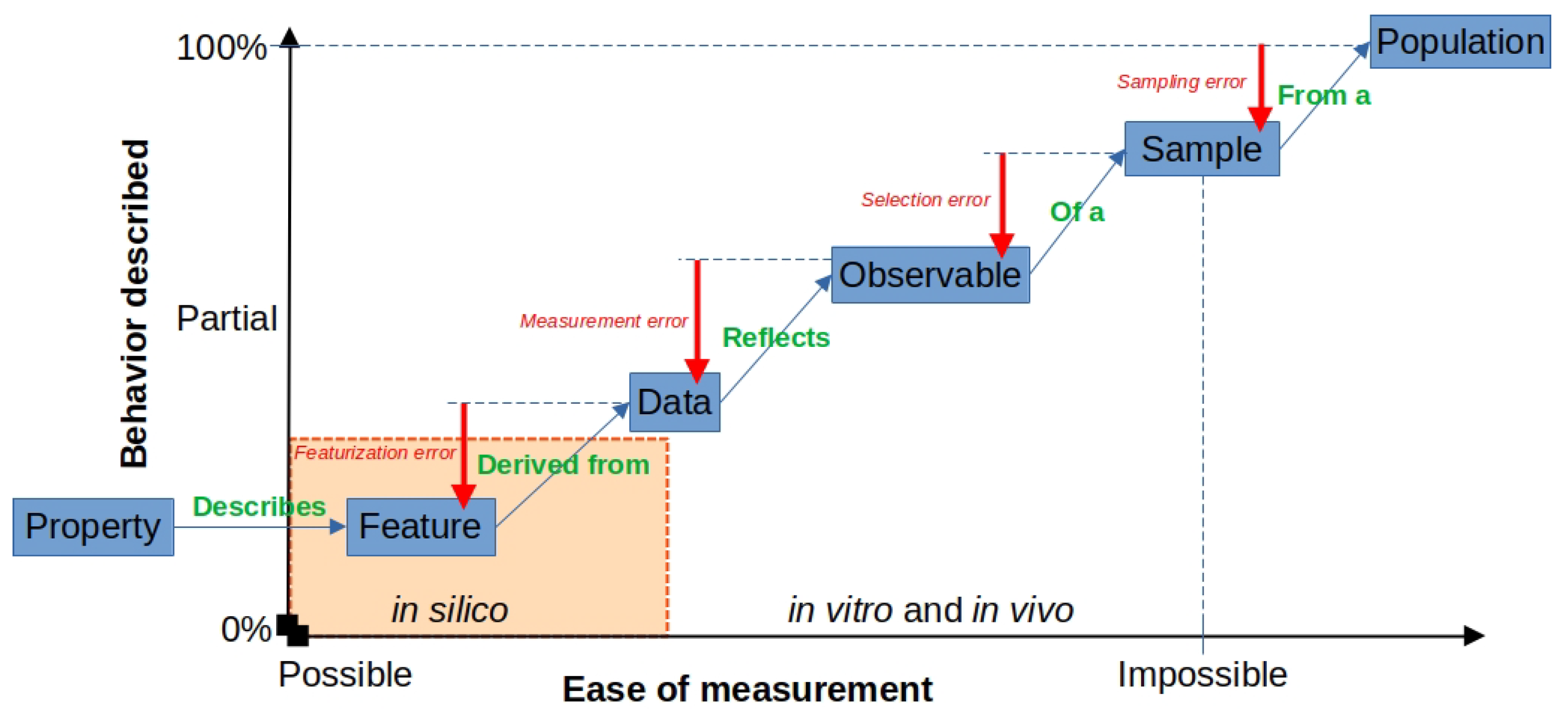
2.3.3. Errors in Feature Engineering from Physical and Computational Sources

In the course of their experiments, scientists may inadvertently redesign existing features, apply them in an inappropriate context, or accrue errors in feature selection that impedes their network training or analysis of results. Several forms of errors arise when features are measured (that is, in vivo or in vitro) and applied (that is, in silico). These errors are generated because features are derived from measurements that are collected using instruments with intrinsic error, because of uncertainties in measuring a sample of matter, or because the feature engineer may not have the essential background information or experience to avoid unintentionally erroneous feature constructions. For molecules, the sample itself is the exact arrangement, dynamics, and quantum uncertainties of all matter within a particular collection. The sample itself is not measurable, but theoretically its exact composition and arrangement contains all possible information (excluding quantum-mechanical uncertainty) about how an experiment on that sample would be consistent with prevailing physical theory—that is, how the sample would behave. Quantum-mechanical uncertainty is presently an irreducible form of error according to Heisenberg’s uncertainty principle, but other errors may be reduced through appropriate mitigation strategies. Each such strategy involves the systematic enumeration, measurement, and reduction of errors. This process might inspire the selection of new experimental reagents, instruments, protocols, algorithms, or analysis methods.
The set of all possible such behaviors are collectively the phenomena that the sample can experience, and observables are produced when these phenomena are measured by any means. First, the sample is collected from a larger population in nature and subjected to controlled experimental conditions, where those phenomena and the values of their observables are influenced by these conditions and the specific sample that was selected. Here, the scientist collects certain measurements designed to capture data reflecting the observables of some material phenomena the scientist expects to measure, although data from other phenomena may also be concomitantly captured. These data are then transformed through the process of “featurization” into features in parallel with hypothesis generation, and these features are subsequently tested by modeling the system of interest. Increasingly, deep learning is the method of choice for such modeling.
However, it is important to remember that these experimentally derived features are products of a sequence of transformations, each of which incurs a unique form of error:
  • When a sample is measured, the particular sample chosen may not be representative of the population from which it is picked, incurring sampling error.
  • The phenomena and its associated observable(s) are necessarily incomplete, because not all observables can be measured, and those that can may not be measurable in isolation from others. Therefore, the selection of which observables to measure incurs selection error.
  • The data may suffer from a low signal-to-noise ratio or reflect measurement error in a sample.
  • During featurization, the scientist might unknowingly neglect useful information, which further convolutes the expected behavior described in the original data, incurring featurization error. This is because the featurization process is dependent on the scientist’s discretion and bias (intended or not) to select valuable information from that dataset.
Thus, all features reflect these four sources of error to some extent. By optimizing each step, the total error can be reduced, but never removed entirely. This concept is illustrated in Figure 3.

2.4. Circumventing Feature-Associated Errors by Systematic Testing

As established in this section, feature selection for a task of interest is an error-prone process. Proper feature selection strengthens the fields’ computational models of reality [34]. The negatives associated with inappropriate feature selection include the following:
  • Existing features are redesigned without insight from previous investigation(s).
  • Features are applied in a context that experts in the field know to be inappropriate.
  • Errors are made in feature selection that impede network training or human insight.
  • Features are implemented in a CPU- or memory-inefficient manner that prevents replication.
Thus, arranging existing features in a taxonomy and developing the means to test them against a panel of analysis or design tasks would serve to benchmark existing features and guide scientists both experimentally and algorithmically. In the current work, we set forth a clear taxonomy that characterizes existing features. We propose that this work, which is currently without code implementations, can be followed naturally by a community-sourced effort to algorithmically implement these features in open-source and scientist-accessible computer code.

3. Methods

3.1. Literature Curation

An extensive literature survey was conducted in order to identify and collect biomolecular features. This meta-analysis was conducted in accordance with the PRISMA guidelines for systematic reviews (Supplementary Figure S1) [35]. First, publications were collected based on literature searches and subsequently filed into one of three Zotero folders broadly based on essential feature type: nonstructural, structural, or dynamical. For each of these folders, a file containing each publication title and metadata was exported and stacked in a single spreadsheet. Then, individual features were extracted from each paper, and columns describing features were manually enumerated. This produced 1360 features, which were individually classified. To preserve context and implementation, deduplication of similar features was not performed. Property columns were then filled for a sample of features across the reported dataset.
In order to collect publications, searches were performed using the Google Scholar literature metasearch engine. A total of 79 publications were initially classified as containing nonstructural features, 305 as containing structural features, and 379 as containing dynamical features. Later, 45 additional papers were added without this prior classification scheme, giving a total of 808 papers. In this study, nonstructural indicated that the examined study focused on fundamental chemical properties and was less reliant on structural or dynamical information; structural indicated the presence of static detail about the arrangement of atoms in three-dimensional space as determined by X-ray crystallography, nuclear magnetic resonance spectroscopy, cryo-electron microscopy, or simulation; and dynamical features contain information about more than one functional state of a molecule or its transitions between states, whether structural or nonstructural. These three groups may be additionally distinguished by their treatment of molecular conformation, that is a specific three-dimensional arrangement of atoms in Cartesian space: “nonstructural” indicates no specific conformations were specified, “structural” indicates at least one was specified with explicit attention to coordinates or equivalent information, and “dynamical” indicates that more than one conformation was specified, albeit not necessarily with coordinates or equivalent information. Structural and dynamical features were given particular attention during our literature search.
After sorting, the papers in these folders were examined, and the features within were extracted, labeled, and classified. Publications were exported into a common file through the Zotero Export menu function. Features were classified with the same labels, nonstructural, structural, and/or dynamical, among other taxa (see Results). Finally, each feature was given both a short and a long name to standardize feature labels and meanings. Because a large number of papers was scanned for features, this metadata is presented in the accompanying feature table rather than appearing as citations in this work. This table can be found on the web at https://github.com/picodase/PREFMoDeL (accessd on 19 February 2023) by navigating to the comma separated value (CSV) file feature_database/features.csv.

3.2. Feature Extraction

Feature extraction was performed using a two-step process. The pdfgrep command-line utility was used to parse through text in each publication for a series of keyphrases. These keyphrases were contained in a plain text file called patterns.txt whose complete contents are shown in Supplementary Figure S2. Some keyphrases were left as incomplete words in order to match a number of possible suffixes. For example, the prefix “featur” can match to both “featurization” and “feature” instead of only one, but is unlikely to match to an off-target word. In order to parse each PDF, the publication hash ID was copied from the common spreadsheet and pasted into Zotero’s search bar at the root “My Library” folder. This returned a single entry with the PDF of interest. Opening this file using the PDF viewer and highlighting the menu bar revealed the PDF file path. An example command run to produce the pdfgrep output was as follows:
pdfgrep -ihnr –context=4 –-file=patterns.txt <PDF_folder>
where the command-line arguments used have the following functions: -i ignores case distinction so as to include upper- and lower-case matches; -h suppresses printing of the filename; -n prints the page number on the left-hand column for ease of location in-text; -r searches the directory recursively for PDFs; and --context=4 yields 4 lines of context before and after a text match. An example output of this function is shown in Figure 4.
The output of pdfgrep was inspected and used to hasten an initial keyword scan, but was not expected to capture all mentioned features. Features were often implicitly defined or encoded in graphs or diagrams which are not visible in the pdfgrep output. Thus, articles containing original features were read for textual references, with special attention to abstracts, introductions, and methods sections. In addition, all figures in each article were examined. In a second pass through the Zotero library, a second set of folders (“nonstructural-2”, “structural-2”, and “dynamical-2”) were constructed and analyzed in the same table. After this analysis, 1360 nondeduplicated features were enumerated. Approximately 700 other tools were collected, including datasets and machine learning architectures, which were not analyzed in this study but are included at the provided GitHub repository. If a feature was presented in a figure or equation, this was enumerated in two columns, where the first indicated the element type (that is, figure, table, or equation) and the second indicated the number of the element from the text (2, 3A, 1B, etc.). Analysis of a sample of this feature set yielded the final taxonomy, where taxa consisted of 45 total properties: 8 categorical properties and 37 binary properties. These properties are defined in the Results section, below.

3.3. Analysis Tools

Properties of features were analyzed using the Orange3 Data Mining suite [36]. Mutually exclusive categorical feature properties were analyzed using pie charts and a percentage table was used to analyze non-mutually exclusive binary properties. Several analyses were performed in Orange3, including general dataset analyses such as property correlation, as well as unsupervised learning techniques such as hierarchical and t-SNE clustering [37,38]. t-SNE was used as an example of a dimensionality-reduction technique to simplify the high-dimensional space (described by 45 feature properties) to a two-dimensional (2D) space. This enables visualizing similarity between features (such as how similar feature X is to Y, or X or Y to Z) based on their Euclidean distance to each other on this 2D space, which is embedded using their enumerated feature properties. Necessarily, analysis of the visualization is highly dependent on the chosen features and the properties by which they are characterized. Plot generation details are provided within the figure captions.

4. Results

Features can be categorized in different ways. Here, we developed an extensible system of classification—a taxonomy—of biomolecular features based on a survey of N = 808 research articles and reviews on proteins and biologically relevant protein-binding ligands. Clearly, this taxonomy can be logically extended to include nucleic acids, carbohydrates, organic compounds, etc.

4.1. Taxonomic Charts

The results of this study are summarized by two tree diagrams, one containing categorical feature properties (Figure 5) and the other containing binary properties (Figure 6).

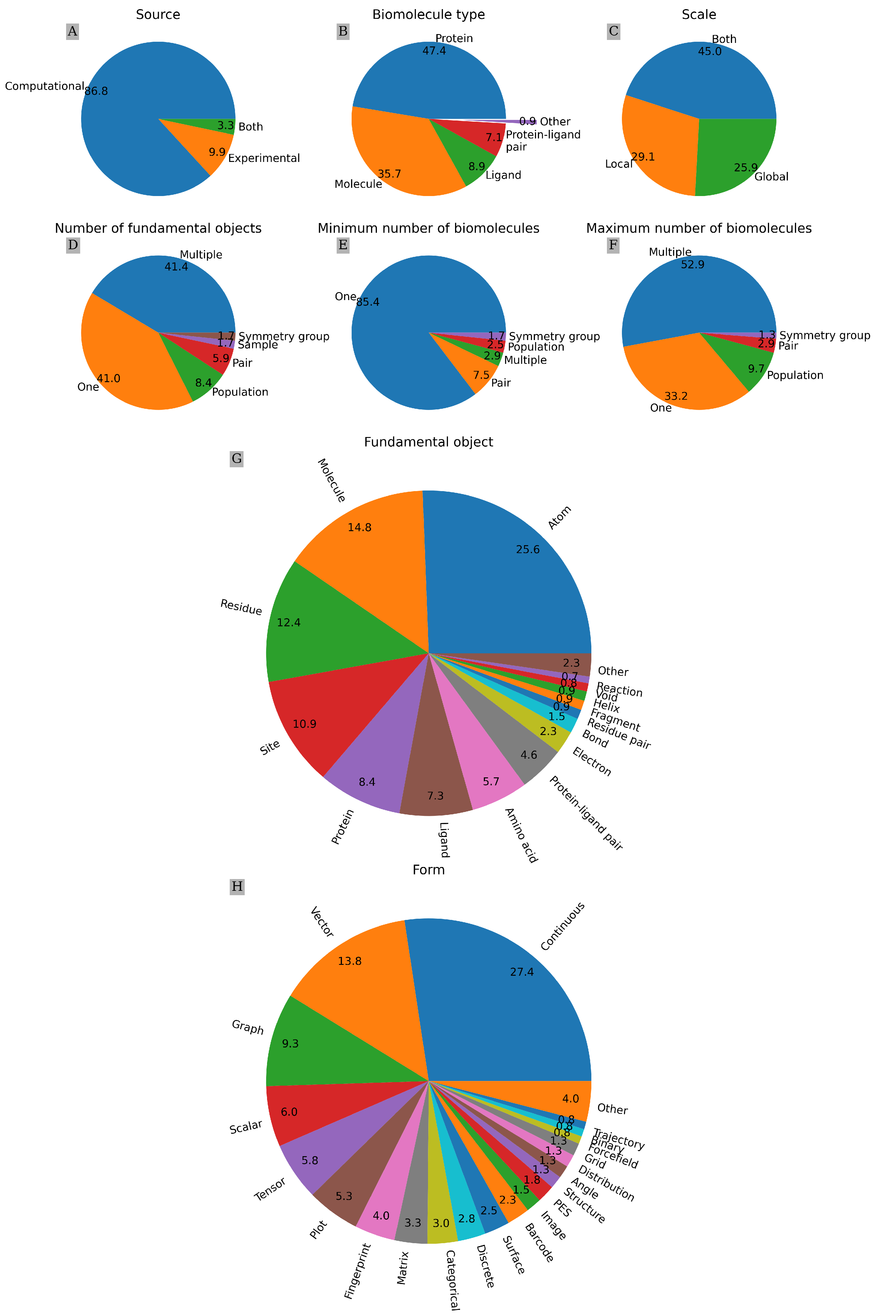
4.2. Categorical Properties

Some evaluated properties were mutually exclusive. Below, these categories are described briefly. Note that biomolecular features are reviewed, in particular features representative of proteins, ligands, and their interactions.
  • Source: Either physical experiment or computational model.
  • Biomolecule type: Protein, ligand, protein–ligand pair, generic molecule, or other.
  • Number of biomolecules: One, pair, multiple, or population. Minimum and maximum number possible to be represented by each feature are counted as separate properties.
  • Fundamental object: Smallest object considered explicitly, e.g., an atom or an amino acid.
  • Number of fundamental objects: One, pair, multiple, symmetry group, sample, or population
  • Form: Data structure, such as a scalar, matrix, or graph.
  • Scale: Local, global, or both.

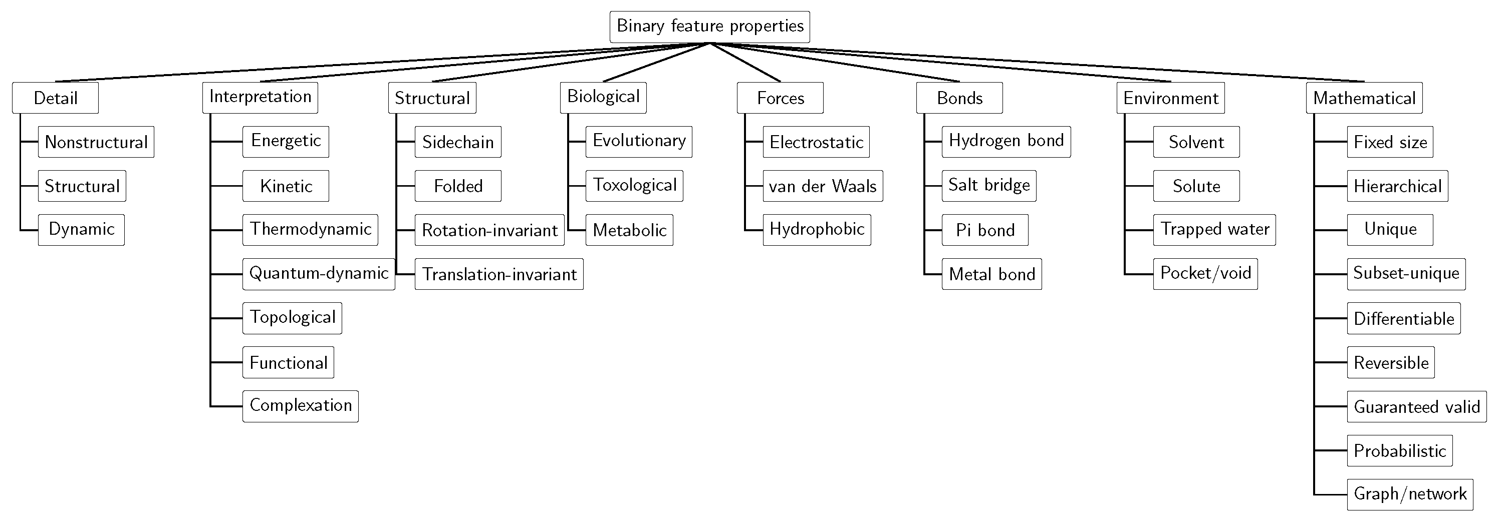
4.3. Binary Properties

Other properties were not mutually exclusive. These properties are grouped and outlined below.
  • Detail: Nonstructural, structural, and dynamical.
  • Interpretation: Energetic, kinetic, thermodynamic, quantum dynamic, topological, functional, and complexation.
  • Structural: Sidechain atoms, macromolecular folding, rotation invariance, and translation equivariance.
  • Biological interpretation: Evolutionary, toxological, and metabolic.
  • Forces: van der Waals, electrostatic, and hydrophobic.
  • Chemical bond: Hydrogen bond, salt bridge, pi bond, and metal bond.
  • Environment: Solvent, solute, trapped waters, and pockets/voids.
  • Mathematical features: Fixed size, hierarchical, unique, subset-unique, differentiable, reversible, guaranteed valid, probabilistic, and graph/network.

4.4. Structural-Feature-Specific Properties

Structural features have one particularly unique property.
  • Structural comparison: Generated by the comparison of two structures, e.g., RMSD.

4.5. Dynamical-Feature-Specific Properties

Dynamical features have several unique properties. Although these were not analyzed in the accompanying table, these were nonetheless observed during the course of feature extraction.
  • Dynamic perspective: State-based or transition-based.
  • Structure set type: Ensemble or trajectory.
  • Probability of dynamics: Most-probable dynamics or rare-event dynamics.
  • Considered states: All states or only relevant states.
  • Period timescale: Thermal noise, functional motion, or evolutionary.
  • Trajectory bias: From a biased simulation, or an unbiased one.

5. Analysis

Pie charts give a property-centric view of the feature dataset. A total of 87% of features are generated through computational means, 10% are generated experimentally, and 3% of features can be generated by either. This reaffirms the assertion that experimental and computational methods are complementary (Figure 7A). Almost half of the features exclusively represent proteins, few exclusively represent ligands, and one-third can represent either biomolecule, which suggests that irrespective of the biomolecule type (that is, protein or ligand), a large selection of features are available (Figure 7B). A plurality of features span both local and global scales, and over a quarter exclusively representing either local or global properties. Thus, surveyed features are robust to multiple scales, where a randomly selected feature is at least 70.9% likely to be able to represent either local or global properties (Figure 7C).
Surveyed features mostly represent one or multiple fundamental objects, with some representing a population of objects, fewer representing a pair of objects, and 1.7% each representing a sample or a symmetry group (Figure 7D). The vast majority of features can represent singular biomolecules, with a few pair-, multiple-, symmetry group-, and population-exclusive features (Figure 7E). Most features can also represent multiple biomolecules, with few exclusively pair- or population-specific features. Only one-third of features can represent at most singular biomolecules, suggesting biomolecule design tasks may make extensive use of the provided feature table (Figure 7F). Although features capable of representing fewer numbers of biomolecules are the majority, the ability to directly represent multiple molecules and populations of molecules is encouraging for biosystem design.
Continuous features constitute a plurality of surveyed features, which makes intuitive sense as structural features are well represented. Furthermore, 50.5% of features either take continuous values, vector form, or graph (network) form (Figure 7H). However, these data are confounded by the form of the feature versus the form of the values within the feature—that is, whether the feature itself is shaped like a matrix, versus the type of value contained at each of its elements (discrete or continuous). In order to better represent feature diversity, these features should be re-classified according to both the form of the feature (feature form) and the form of the values within the feature (numerical form), as applicable. The fundamental objects represented by each feature are more diverse, with the most common fundamental object, atoms, only composing twenty-six percent of the feature set, followed by molecules, residues (either an amino acid or a nucleic acid base pair), binding sites, proteins, ligands, amino acids, and protein–ligand pairs (Figure 7G).
Binary feature properties are outlined in Table 1, which also provides a property-centric view of the feature dataset. Features with a structural interpretation constitute the majority of features at 65%, while nonstructural and dynamic interpretations are less common. A majority of features can represent molecular topology and complex formation, but very few measure either quantum-dynamic or evolutionary detail. This suggests that features capable of representing these properties are excellent targets for new investigations.
More features are rotationally and translationally invariant than those which had structural detail, which is reasonable as structural-detail-containing features are the most likely to depend on rotations and translations. Thus, it is expected that rotational and translational invariance is concentrated in molecules without a structural representation. Recent work has produced architectures capable of learning from features with rotational and translational equivariance [39], such as the SE(3) transformer [40], so these issues with many structural features are not insurmountable. Fewer features are capable of representing amino acid sidechains, which correlates with a presence of global structural analyses that subselected alpha-carbon atoms from a larger protein structure, while neglecting amino acid side chains. This is useful for global structural or dynamical features, but less so for features describing molecular interactions (binding or enzymatic). However, as sidechain-scale local dynamical features are developed for faster biomolecular rearrangements, this difference should diminish (Table 1).
Approximately one-quarter of features represent forces of any kind, which are likely to be concentrated in features with dynamic representations. Bond types are far more variable, with hydrogen bonds and salt bridges being most commonly represented in one-third of features, with pi bonds being least represented at fewer than one-fifth. This disparity signifies greater attention applied to hydrogen bonds, which is generally true in the field due to their known importance in secondary structure, stabilization of internal protein structure, solvent interactions, and ligand binding. By contrast, pi bonds and metal bonds are far less common. As more precise structural and dynamical methods are developed, these types of interactions should gain more attention (Table 1).
Approximately half of features are capable of representing environmental features such as solvent, solute, and pockets. Trapped water-capable representations are less represented in the dataset, as they required not only the appropriate experimental structural detail but also solvent representation, among other details (Table 1).
Among the mathematical properties surveyed, features are most commonly guaranteed to be valid representations. This is expected, as many analysis algorithms give deterministic output generated from extensively validated static experimental data (such as crystal structures from the PDB [41] and PDBBind [42]), while by contrast experimental methods often require specialized skills. Some computational methods are not guaranteed to be valid, such as biased sampling molecular simulations. For example, over 40% of features are of fixed dimensions or can represent detail hierarchically. The least commonly satisfied properties are subset uniqueness, which is only guaranteed with certain latent space representations from neural networks. Reversibility is often lost because many features concentrate on the most relevant parts of a dataset while ignoring other aspects of an experiment. Only one-third of features can be interpreted probabilistically, which is highly represented with dynamical and reduced structural features (Table 1).
Correlated properties (Table 2) tend to fall pairwise into three groups: mathematical, interactions (including forces and bonds), and environment. These results are easily rationalized because features describing bonds tend to describe many types of bonds, rotationally invariant metrics are almost always translationally invariant, and features describing energetic detail are closely related with bonds and environment. An interesting correlation is between reversibility and subset-uniqueness. This may be rationalized because reversible transformations compress essential information into a secondary space, such that all parts of the transformed space are sufficiently unique to distinguish the elements in the untransformed space.
Qualitative analysis of two-dimensional t-SNE plots of the feature database (Figure 8) revealed that dynamically capable features tend to reside in a corner of the space, the area shown with the yellow background in Figure 8, and that more dynamically capable features are also capable of representing complexes. This conclusion is interesting because complex-capability appears slightly enriched in dynamically capable representations, but is ultimately not surprising because complex formation is a dynamic process being extensively studied by a large number of research groups.
Features capable of representing bonding cluster on the right-hand side of the t-SNE plot (Supplementary Figure S3). As protein-representing features are concentrated on the bottom of the figure, this suggests that the majority of protein-capable features do not explicitly represent bonding. This implies that gross structural features are often preferred to specific local interactions in the existing set of structural features. Because local bonding is essential to biomolecular function, it should be emphasized in new features where appropriate.
A final visualization of the same space (Supplementary Figure S4) suggests that structurally capable features occupy the right-hand side of the space, and that they are distributed over more of the feature space. Features representing structure are far more likely to represent complexation than nonstructural features. This is reasonable as protein–ligand complexes cannot be richly represented by metrics which ignore structure.

6. Discussion

6.1. A Note on Feature Characterization Error

Error in feature characterization may arise from an ambiguous or alternate interpretation of implicit features. Implicit features are those that are assumed to exist by scientists familiar with a particular subfield, and may or may not be discussed verbally by practitioners in the laboratory setting, and are not explicitly mentioned (written, graphical, or subtext) in the scientific literature [50,51]. While explicit features are described through a formula, definition, figure, or algorithm, often with an accompanying value proposition that specifies the feature’s properties, implicit features were harder to characterize. They perhaps contributed to the appearance of a figure, but were not strongly emphasized in the text. It is possible that these features could be learned by a deep learning model through representation learning, and therefore the characterization of all implicit features would be a low-priority task for the field. Work in semantic analysis suggests that language models are capable of identifying implicit features [52]. Lacking the specific knowledge of each subfield from which the literature was surveyed in this study, it is very likely that some features required deeper knowledge and that feature characterization accuracy was concomitantly reduced. By consulting experts with years of experience in the techniques of crystallography or quantum chemistry, this characterization accuracy would be raised significantly. Supplementary Figure S5, which is analogous to Figure 3, illustrates the forms of error incurred as methods were applied to collect features.

6.2. Directions for Future Work

6.2.1. Feature Relevance

This study was conducted with the assumption that all features collected are equally useful for the particular task they were designed for. Thus, in the current iteration of this feature table, no feature relevance metrics are applied, which precluded supervised learning on the table to draw some insights. In future iterations of this table, the performance of specific design tasks for specific molecules should be tabulated for each feature. This would enable ablation studies on the feature property dataset, unveiling how individual features or combinations of features help molecular analysis and design. Outside metrics can also be used, such as the Comparative Assessment of Scoring Functions (CASF) [53] or AlphaFold [7] can be used to judge protein–ligand complexes.

6.2.2. Underrepresented Taxa

Through the course of collecting features and analyzing the resulting table of biomolecular features, we recognized that several properties of features in the taxonomy are underrepresented. These areas warrant further attention, and several examples are given below.
  • Residue-Specific Atomic Subsets. Previous work by Cang and Wei included three atomic structural partitions [54]. In one representation, they included the entire structure for atom partitioning, in a second representation they only included primary and secondary shell residues in the binding site, and in a third representation they selected subsets representing the interactions between two atomic elements. However, this approach excludes allosteric networks and amino acid level properties. To alleviate this unintended bias, scientists should partition structures by residue properties and by computationally or experimentally elucidated allosteric residue interaction networks.
  • Amino acid specific features. Currently, few amino acid specific representations exist, thus this is a major growth area for protein-specific structural dynamic features. As mentioned, amino acid motion (and their restriction, such as in active site preorganization) is essential for protein function, although without the tools to experimentally measure amino acid motion, insights cannot be drawn from amino acid dynamics. New features should address amino acid specific dynamics, and extend these dynamic models beyond the common but rudimentary Principal Component Analysis (PCA) to describe more complex motions with simple equations.
  • Structural trajectories: “dynamicalization” of structural features. It would be computationally trivial to expand all structural features to dynamic structural features through molecular dynamics simulation. Recent work has improved the efficiency and analysis of these simulations by integration with DL modeling [55,56] and given guidance to practitioners for which models they should use with their systems of study [57].
  • Evolutionary trajectories. In order to make evolutionary methods more accessible and useful and to take advantage of existing evolutionary knowledge, many desired features can be computed along an evolutionary trajectory. This is accessible for most computational methods and may be powerfully applied to evolutionary design tasks.

6.2.3. Deduplication and Expansion of Feature Properties

While compiling features for our dataset, we recognized that some of the features are repeated, but did not prune these duplicated features in order to not lose the context in which these features were applied and their specific method of implementation. We acknowledge that in the absence of deduplication the analysis of feature relevance, feature ubiquity across different design tasks, and/or historical trends in features is hindered. We also recognize that unintended bias is also present not only in which features were extracted from selected publications, but also in the collection of columns used to classify feature properties, making the accurate assessment of feature properties difficult. For these reasons, we strongly feel that community-sourced involvement should yield a more systematic column selection and grouping, ultimately yielding multiple levels of insight into feature relevance for molecular modeling and design. Thus, future iterations of this dataset will presumably classify features more exactly.

6.2.4. Potential New Features for Molecular Deep Learning

This current meta-analysis of biomolecular features for deep learning presents a broad perspective on specific features utilized in publications across the field of biochemistry. The primary goal for developing our taxonomy was to organize the current state of the art of biomolecular features for deep learning to strengthen future implementations of deep learning models to the wide variety of biochemical, molecular interaction, and biomedical questions being studied by research investigators worldwide. After our analysis, we discovered that the resulting taxonomy of features also served to highlight several noticeable voids in the molecular feature space, especially with respect to dynamic structural features. A few examples of potential new features are described below. Furthermore, these features should be, in principle, relatively straightforward to implement using modern Python libraries.
  • Kinetics-Weighted and Multi-Transition State Sequences. The consensus structure method described by Smith et al. [58] is an excellent advance in enzyme design, but can be slightly modified to incorporate more dynamic detail. Each transition state’s contribution can be weighted by the inverse of the experimentally determined forward kinetic constant for that particular reaction step. This adjustment would enable the slowest reaction barriers to exert the greatest influence on the consensus structure. Secondly, multiple transition states might be considered rather than creating a consensus structure. This can be accomplished by optimizing multiple states and their transitions by using fast protein motions, such as sidechain rearrangements, cofactor vibrations, and other atom-scale dynamics. These two features, coupled with methods developed to utilize them to the fullest extent, would enhance structure- and dynamics-based enzyme engineering efforts.
  • Bond strain vector. A bond strain vector would describe bond strain for every bond in a protein or ligand from theoretically ideal values. Such a feature can be visualized as a one-dimensional vector where each index in the vector holds the energy of the indexed bond in kilojoules per mole. Through application of Hooke’s law and idealized bond geometries, bond energy deviations are easily computed. Then, they can be visualized on a protein structure, or for a ligand, bound in an active site. Such a feature is extensible to analogues for angular strain (between three atoms) or torsional strain (between four atoms) which together describe the system in more dynamic and mechanical detail. This feature would illustrate where strain is present in a protein or a ligand structure and may prove important in deep learning tasks concerning function such as recognition, binding, and catalysis [59].
  • Amino acid sidechain normal modes. Conformational plasticity, from high-frequency rate-promoting vibrations to sidechain rotamer sampling to large domain motion, is often required to understand protein function [60,61,62,63]. This is especially relevant on the scale of individual amino acid sidechains within a binding pocket, as they are often subject to rapid structural rearrangements to enable precise biochemical function. Bonk et al. simulated enzyme active site dynamics with restricted conformational mobility to determine which structural features activate catalysis [64]. The ability to compute other such elementary features may lead to widely interpretable insight when applied to novel systems. For example, single amino acid motions are critical for the substrate IP7 to enter the active site of PPIP5K2. Here, a single residue glutamine-192 utilizes spontaneous motion and the irreversibility of reverse substrate diffusion to ratchet IP7 from a capture site to the active site [65]. These case studies demonstrate the value of the automatic extraction of this detail to sense amino acid motions for analysis or design purposes. While alpha carbon PCA is a popular model to enable quick visually interpretable dynamic structural features for a gross protein structure traveling through an ensemble or trajectory [66], no analogous feature exists for substructures such as sidechains within the protein. In order to compute such a feature, one would fix a reference frame at each alpha carbon and measure wagging or spinning modes for each amino acid along with their frequencies using PCA or nonlinear dimensionality reduction techniques. Next, these modes could be projected onto the larger protein structure and analyzed for their correspondence with the more slowly relaxing backbone modes produced by alpha carbon PCA. These collections of principal components can then be used to construct features assuming either independence of motion or any particular dependence, based on correlations in molecular dynamics trajectories or NMR-derived ensembles. By repeating this process for all non-glycine amino acids in a structure, these “amino acid sidechain normal modes” could reveal how sums of large and small dynamic principal components enable protein function on multiple scales.
  • Docking strength for interaction specificity and uniqueness. Specificity in biomolecular recognition and binding is a composite problem involving the maximization of on-target interactions and minimization of off-target ones. Because so many off-target molecules exist in the cell, this is challenging to solve analytically. However, methods that measure the strength of binding between two proteins raise the potential to initiate examination of this space. Such a method could be docking-based, but may be efficiently implemented by using DL to reduce docking strength determination to a sequence of matrix multiplications. Using such a method, ostensibly a “kinetic association constant regressor network”, off-target interactions could be minimized for each non-target endogenous protein, while on-target interactions would be maximized. Such a solution would be a first step towards minimizing unintentional drug side effects without requiring manual testing of all possible cross interactions in the cell.

6.2.5. Automated Feature Engineering and the Need for Functional Data

Representation learning combines human-readable hand-crafted features into high-dimensional, machine-readable composite features [67,68]. Critically, these composite features are constrained by the input data and representative power of the network, and therefore must be built from rigorous, representative elementary features that span all aspects of relevant biomolecular function. Because there is currently insufficient functional data (binding constants, enzyme kinetics, spectroscopies, etc.) to train DL networks to relate an arbitrary ligand or protein structure to its function, this space is still sparsely explored. Thus, while automated feature engineering may judge feature relevance, hand-crafted features remain relevant.

6.2.6. Unsupervised Learning Visualization for Dataset Exploration

As researchers explore the feature dataset, using interactive tools to visualize the feature set will facilitate their selection of properties—and subsequently the features—that are most relevant to their own analyses and design tasks, and their integration into their own deep learning models. The t-SNE visualization shown in Figure 8 is a statistically meaningful way to embed high-dimensionality data (as is present in the feature dataset) into a more readily interpretable two- or three-dimensional map. By judiciously using color, size, and outlines, even more dimensions are accessible. This visualization allows the researcher to leverage the feature space for their own task.

6.2.7. Feature Implementations and Future Integrations

Existing software packages have made selected feature sets available for specific types of biomolecules. Specifically, the DeepChem drug discovery feature library DeepChem [69] provides feature conversions for ligand systems, and the Graphein library [70] already includes many graph-based protein features. A broader library could be written for all described features and diverse molecule types, with each feature classified according to their properties. Implementing the complete list as presented in the feature table is beyond the scope of this work, and would benefit immensely from community-level discussion of optimal approaches for development. It remains an open project to collect this library of open-source implementations with an accessible and appropriate API for end-users.
Keeping this essential database up-to-date is envisioned as a community-based task that benefits significantly from the open-source development model. Sharing the task of collection, implementation, and analysis of features, would materialize several key benefits. Firstly, the task of collection and analysis would not fall on a single person, which enables the project to extend beyond the time and effort constraints of that person. Second, the perspectives represented in the table would be averaged between the contributors and thus reduce intrinsic or unintentional biases. Thirdly, feature evaluation and opt-in performance telemetry could be used to analyze feature relevance by measuring which features or collection of features perform best in specific tasks [28,30,34,71]. Existing algorithms [72,73] and software [74,75] are already implemented and capable of using such telemetry for automated calculation of feature relevance, or to aid investigators in their search for optimal features [76].
Eventually, such a database of features could be integrated into established molecular simulation suites. One notable example is Omnia, which uses the package OpenMM for molecular dynamics trajectory generation, MDTraj [77] for molecular dynamics trajectory analysis, TorchMD [56] for improved efficiency in molecular simulation, MSMBuilder2 [78] and PyEMMA [79] for the construction of Markov State Models, and YANK for alchemical free energy calculations. Another package called ProDy [66] includes several features documented in the features table. Similar integrated feature modeling suites could automatically generate robust existing features and enable easier implementations for new compound features. Finally, integration into protein modeling software suites such as Rosetta would bring these insights directly to protein designers.

6.2.8. Publicly Available Biophysical Datasets

Compiling datasets from biophysical assays has become a more common practice with improvements in experimental techniques, software, and hardware over recent decades. Because features are designed using empirical data, rigorous and auditable feature implementations require the data to be publicly available. Plentiful publicly available image and text data were used to train Stable Diffusion [80] and ChatGPT [81], respectively, which define the state of the art in their tasks. In the biophysical literature, open data have already led to the creation of powerful deep learning models such as AlphaFold [7] and RoseTTAFold [6] from the Protein Data Bank (PDB) [41], RGN2 [82] from the UniParc protein sequence database [83], cryoDRGN [84] from the EMPIAR database [85], and ModelAngelo [86] from the Electron Microscopy Database (EMDB) [87]. Similarly vast biophysical databases are poised to be incorporated into useful data-driven deep learning models to glean dynamical details, such as NMR chemical shift data from the Biological Magnetic Resonance Database (BMRB) [88] or Small Angle Scattering Biological Data Bank (SASBDB) [89].
As deep learning has grown in popularity, more public databases of biophysical observables have been created on the worldwide web. We support this trend, and encourage the reader to submit their data to these public databases or to create these public databases with their colleagues if they do not already exist. The overall range of benefits of this work are hard to predict, but several are easily anticipated. Beyond structural dynamics, functional data from databases containing binding constants [42], enzyme mechanisms [90], and enzyme activity measurements [91], or electronic data from biomolecular FRET, EPR, and Raman spectroscopies could enable direct analysis and design of quantum states in enzyme active sites, a prevailing grand challenge even with the advent of structural deep learning networks.

7. Conclusions

A list of 1360 nonunique observed biomolecular features was extracted from N = 808 publications and classified by a series of feature properties. Feature properties were generalized to produce a taxonomy of biomolecular features. Feature space was visualized using compositional pie charts and unsupervised clustering methods in order to explore and describe feature space topology. New features were proposed using this taxonomy as a guide which would serve to fill some voids not currently addressed in the literature. Finally, directions for further development of the feature table with a mechanism for analyzing each feature’s efficacy in analysis and design tasks were discussed, and the benefits of implementing these features in an open sourced, public repository were outlined.

Supplementary Materials

The following supporting information can be downloaded at https://www.mdpi.com/article/10.3390/app13074356/s1, Figure S1: The PRISMA 2020 flow diagram for the meta-analysis of biomolecular features; Figure S2: Contents of patterns.txt; Table S1: A table of mathematically-ideal properties and their significance; Table S2: Table of terms used in literature metasearch sorted by feature type; Figure S3: Feature clustering by t-SNE using biomolecule type and ability to represent bonding; Figure S4: Feature clustering by t-SNE using the ability to represent structure and molecular complexes; Figure S5: Conceptual relation of six types of data-containing objects used in feature collection.

Author Contributions

Conceptualization: J.L.N. and V.L.H.; methodology: J.L.N.; data curation: J.L.N.; analysis: J.L.N.; supervision: V.L.H.; writing—original draft preparation: J.L.N.; writing—review, editing, and finalizing: V.L.H.; funding acquisition: V.L.H. All authors have read and agreed to the published version of the manuscript.

Funding

This work was supported in part by NIGMS grant number 1R02GM140183 (Christopher Beaudry, P.I.) and an OSU/CoS Summer Undergraduate Research Experience (SURE) Award.

Data Availability Statement

The full feature dataset can be found at the URL https://github.com/picodase/PREFMoDeL (accessd on 19 February 2023). The table can be viewed by navigating to the feature_database/features.csv CSV file. In addition, the Orange3 session file and several jupyter notebooks providing basic statistics about the dataset are included in this repository. A folder structure for future feature implementations is also included at this address.

Acknowledgments

We thank P. Andrew Karplus for insightful discussion supporting this work in its early stages. Any opinions, findings, conclusions, or recommendations expressed in this manuscript are those of the authors and do not necessarily reflect the views of the National Institutes of Health.

Conflicts of Interest

The authors declare no conflict of interest.

Abbreviations

The following abbreviations are used in this manuscript:
AIArtificial Intelligence
APIApplication Programming Interface
BMRBinding Mode Representation
BMRBBiological Magnetic Resonance Database
CASFComparative Assessment of Scoring Functions
CCECategorical Cross Entropy
CNNConvolutional Neural Network
CPUCentral Processing Unit
CSVComma Separated Value
DLDeep Learning
DRINDynamic Residue Interaction Network
EMDBElectron Microscopy Database
EMPIARElectron microscopy public image archive
EPRElectron Paramagnetic Resonance
FRETFörster Resonance Energy Transfer
GNNGraph Neural Network
MDMolecular Dynamics
MLMachine Learning
NDn-Dimensional
PCAPrincipal Component Analysis
PDBProtein Data Bank
PDFPortable Document Format
PREFMoDeLPublic Repository of Engineered Features for Molecular Deep Learning
SASBDBSmall Angle Scattering Biological Data Bank
SGDStochastic Gradient Descent
SWIFSurface-Weighted Interaction Fingerprint
t-SNE             t-distributed Stochastic Neighbor Embedding
URLUniform Resource Locator

References

  1. Drews, J. Drug Discovery: A Historical Perspective. Science 2000, 287, 1960–1964. [Google Scholar] [CrossRef]
  2. Vincent, F.; Nueda, A.; Lee, J.; Schenone, M.; Prunotto, M.; Mercola, M. Phenotypic drug discovery: Recent successes, lessons learned and new directions. Nat. Rev. Drug Discov. 2022, 21, 899–914. [Google Scholar] [CrossRef]
  3. Dara, S.; Dhamercherla, S.; Jadav, S.S.; Babu, C.M.; Ahsan, M.J. Machine Learning in Drug Discovery: A Review. Artif. Intell. Rev. 2022, 55, 1947–1999. [Google Scholar] [CrossRef] [PubMed]
  4. Schneider, P.; Walters, W.P.; Plowright, A.T.; Sieroka, N.; Listgarten, J.; Goodnow, R.A.; Fisher, J.; Jansen, J.M.; Duca, J.S.; Rush, T.S.; et al. Rethinking drug design in the artificial intelligence era. Nat. Rev. Drug Discov. 2020, 19, 353–364. [Google Scholar] [CrossRef] [PubMed]
  5. Long, A.a.W.; Nayler, J.H.C.; Smith, H.; Taylor, T.; Ward, N. Derivatives of 6-aminopenicillanic acid. Part XI. α-Amino-p-hydroxybenzylpenicillin. J. Chem. Soc. Org. 1971, 1920–1922. [Google Scholar] [CrossRef]
  6. Baek, M.; DiMaio, F.; Anishchenko, I.; Dauparas, J.; Ovchinnikov, S.; Lee, G.R.; Wang, J.; Cong, Q.; Kinch, L.N.; Schaeffer, R.D.; et al. Accurate prediction of protein structures and interactions using a three-track neural network. Science 2021, 373, 871–876. [Google Scholar] [CrossRef]
  7. Jumper, J.; Hassabis, D. Protein structure predictions to atomic accuracy with AlphaFold. Nat. Methods 2022, 19, 11–12. [Google Scholar] [CrossRef]
  8. Dauparas, J.; Anishchenko, I.; Bennett, N.; Bai, H.; Ragotte, R.J.; Milles, L.F.; Wicky, B.I.M.; Courbet, A.; Haas, R.J.d.; Bethel, N.; et al. Robust deep learning based protein sequence design using ProteinMPNN. Science 2022, 378, 49–56. [Google Scholar] [CrossRef]
  9. Arunachalam, P.S.; Walls, A.C.; Golden, N.; Atyeo, C.; Fischinger, S.; Li, C.; Aye, P.; Navarro, M.J.; Lai, L.; Edara, V.V.; et al. Adjuvanting a subunit COVID-19 vaccine to induce protective immunity. Nature 2021, 594, 253–258. [Google Scholar] [CrossRef] [PubMed]
  10. Peón, A.; Naulaerts, S.; Ballester, P.J. Predicting the Reliability of Drug-target Interaction Predictions with Maximum Coverage of Target Space. Sci. Rep. 2017, 7, 3820. [Google Scholar] [CrossRef]
  11. Cerisier, N.; Petitjean, M.; Regad, L.; Bayard, Q.; Réau, M.; Badel, A.; Camproux, A.C. High Impact: The Role of Promiscuous Binding Sites in Polypharmacology. Molecules 2019, 24, 2529. [Google Scholar] [CrossRef] [PubMed]
  12. Blaschke, T.; Feldmann, C.; Bajorath, J. Prediction of Promiscuity Cliffs Using Machine Learning. Mol. Informatics 2021, 40, 2000196. [Google Scholar] [CrossRef] [PubMed]
  13. Feldmann, C.; Bajorath, J. Machine learning reveals that structural features distinguishing promiscuous and non-promiscuous compounds depend on target combinations. Sci. Rep. 2021, 11, 7863. [Google Scholar] [CrossRef]
  14. Gilberg, E.; Gütschow, M.; Bajorath, J. Promiscuous Ligands from Experimentally Determined Structures, Binding Conformations, and Protein Family-Dependent Interaction Hotspots. ACS Omega 2019, 4, 1729–1737. [Google Scholar] [CrossRef] [PubMed]
  15. Wigh, D.S.; Goodman, J.M.; Lapkin, A.A. A review of molecular representation in the age of machine learning. Comput. Mol. Sci. 2022, 12, e1603. [Google Scholar] [CrossRef]
  16. Friederich, P.; Krenn, M.; Tamblyn, I.; Aspuru-Guzik, A. Scientific intuition inspired by machine learning-generated hypotheses. Mach. Learn. Sci. Technol. 2021, 2, 025027. [Google Scholar] [CrossRef]
  17. Gu, J.; Wang, Z.; Kuen, J.; Ma, L.; Shahroudy, A.; Shuai, B.; Liu, T.; Wang, X.; Wang, G.; Cai, J.; et al. Recent advances in convolutional neural networks. Pattern Recognit. 2018, 77, 354–377. [Google Scholar] [CrossRef]
  18. Wu, Z.; Pan, S.; Chen, F.; Long, G.; Zhang, C.; Yu, P.S. A Comprehensive Survey on Graph Neural Networks. IEEE Trans. Neural Networks Learn. Syst. 2021, 32, 4–24. [Google Scholar] [CrossRef]
  19. Vaswani, A.; Shazeer, N.; Parmar, N.; Uszkoreit, J.; Jones, L.; Gomez, A.N.; Kaiser, L.; Polosukhin, I. Attention Is All You Need. arXiv 2017, arXiv:1706.03762. [Google Scholar]
  20. Wang, Z.; Liu, M.; Luo, Y.; Xu, Z.; Xie, Y.; Wang, L.; Cai, L.; Qi, Q.; Yuan, Z.; Yang, T.; et al. Advanced graph and sequence neural networks for molecular property prediction and drug discovery. Bioinformatics 2022, 38, 2579–2586. [Google Scholar] [CrossRef]
  21. Fang, X.; Liu, L.; Lei, J.; He, D.; Zhang, S.; Zhou, J.; Wang, F.; Wu, H.; Wang, H. Geometry-enhanced molecular representation learning for property prediction. Nat. Mach. Intell. 2022, 4, 127–134. [Google Scholar] [CrossRef]
  22. Wang, Q.; Ma, Y.; Zhao, K.; Tian, Y. A Comprehensive Survey of Loss Functions in Machine Learning. Ann. Data Sci. 2022, 9, 187–212. [Google Scholar] [CrossRef]
  23. Ciampiconi, L.; Elwood, A.; Leonardi, M.; Mohamed, A.; Rozza, A. A survey and taxonomy of loss functions in machine learning. arXiv 2023, arXiv:2301.05579. [Google Scholar]
  24. Chauvin, Y.; Rumelhart, D.E. (Eds.) Backpropagation: Theory, Architectures, and Applications; Psychology Press: London, UK, 1995. [Google Scholar] [CrossRef]
  25. Lillicrap, T.P.; Santoro, A.; Marris, L.; Akerman, C.J.; Hinton, G. Backpropagation and the brain. Nat. Rev. Neurosci. 2020, 21, 335–346. [Google Scholar] [CrossRef] [PubMed]
  26. Abdolrasol, M.G.M.; Hussain, S.M.S.; Ustun, T.S.; Sarker, M.R.; Hannan, M.A.; Mohamed, R.; Ali, J.A.; Mekhilef, S.; Milad, A. Artificial Neural Networks Based Optimization Techniques: A Review. Electronics 2021, 10, 2689. [Google Scholar] [CrossRef]
  27. AlQuraishi, M.; Sorger, P.K. Differentiable biology: Using deep learning for biophysics-based and data-driven modeling of molecular mechanisms. Nat. Methods 2021, 18, 1169–1180. [Google Scholar] [CrossRef]
  28. König, G.; Molnar, C.; Bischl, B.; Grosse-Wentrup, M. Relative Feature Importance. In Proceedings of the 25th International Conference on Pattern Recognition (ICPR), Milan, Italy, 10–15 January 2021; pp. 9318–9325. [Google Scholar] [CrossRef]
  29. Dhal, P.; Azad, C. A comprehensive survey on feature selection in the various fields of machine learning. Appl. Intell. 2022, 52, 4543–4581. [Google Scholar] [CrossRef]
  30. Bouchlaghem, Y.; Akhiat, Y.; Amjad, S. Feature Selection: A Review and Comparative Study. E3S Web Conf. 2022, 351, 01046. [Google Scholar] [CrossRef]
  31. Noé, F.; Tkatchenko, A.; Müller, K.R.; Clementi, C. Machine Learning for Molecular Simulation. Annu. Rev. Phys. Chem. 2020, 71, 361–390. [Google Scholar] [CrossRef]
  32. Haghighatlari, M.; Li, J.; Heidar-Zadeh, F.; Liu, Y.; Guan, X.; Head-Gordon, T. Learning to Make Chemical Predictions: The Interplay of Feature Representation, Data, and Machine Learning Methods. Chem 2020, 6, 1527–1542. [Google Scholar] [CrossRef]
  33. George, J.; Hautier, G. Chemist versus Machine: Traditional Knowledge versus Machine Learning Techniques. Trends Chem. 2021, 3, 86–95. [Google Scholar] [CrossRef]
  34. Kumar, V.; Minz, S. Feature Selection: A Literature Review. Smart Comput. Rev. 2014, 4, 211–229. [Google Scholar] [CrossRef]
  35. Liberati, A.; Altman, D.G.; Tetzlaff, J.; Mulrow, C.; Gøtzsche, P.C.; Ioannidis, J.P.A.; Clarke, M.; Devereaux, P.J.; Kleijnen, J.; Moher, D. The PRISMA statement for reporting systematic reviews and meta-analyses of studies that evaluate healthcare interventions: Explanation and elaboration. BMJ 2009, 339, b2700. [Google Scholar] [CrossRef] [PubMed]
  36. Demšar, J.; Curk, T.; Erjavec, A.; Črt Gorup; Hočevar, T.; Milutinovič, M.; Možina, M.; Polajnar, M.; Toplak, M.; Starič, A.; et al. Orange: Data Mining Toolbox in Python. J. Mach. Learn. Res. 2013, 14, 2349–2353. [Google Scholar]
  37. Hinton, G.E.; Roweis, S. Stochastic Neighbor Embedding. In Advances in Neural Information Processing Systems; MIT Press: Cambridge, MA, USA, 2002; Volume 15, pp. 857–864. [Google Scholar]
  38. Maaten, L.v.d.; Hinton, G. Visualizing Data using t-SNE. J. Mach. Learn. Res. 2008, 9, 2579–2605. [Google Scholar]
  39. Miller, B.K.; Geiger, M.; Smidt, T.E.; Noé, F. Relevance of Rotationally Equivariant Convolutions for Predicting Molecular Properties. arXiv 2020, arXiv:2008.08461. [Google Scholar]
  40. Fuchs, F.B.; Worrall, D.E.; Fischer, V.; Welling, M. SE(3)-Transformers: 3D Roto-Translation Equivariant Attention Networks. In Proceedings of the 34th International Conference on Neural Information Processing Systems, Vancouver, BC, Canada, 6–12 December 2020; pp. 1970–1981. [Google Scholar]
  41. Berman, H.M.; Westbrook, J.; Feng, Z.; Gilliland, G.; Bhat, T.N.; Weissig, H.; Shindyalov, I.N.; Bourne, P.E. The Protein Data Bank. Nucleic Acids Res. 2000, 28, 235–242. [Google Scholar] [CrossRef]
  42. Liu, Z.; Li, Y.; Han, L.; L, J.; Liu, J.; Zhao, Z.; Nie, W.; Yuchen, L.; Wang, R. PDB-wide Collection of Binding Data: Current Status of the PDBbind Database. Bioinformatics 2014, 31, 405–412. [Google Scholar] [CrossRef]
  43. Bourgeat, L.; Serghei, A.; Lesieur, C. Experimental Protein Molecular Dynamics: Broadband Dielectric Spectroscopy coupled with nanoconfinement. Sci. Rep. 2019, 9, 17988. [Google Scholar] [CrossRef]
  44. Pradeepkiran, J.; Reddy, P. Structure Based Design and Molecular Docking Studies for Phosphorylated Tau Inhibitors in Alzheimer’s Disease. Cells 2019, 8, 260. [Google Scholar] [CrossRef]
  45. Fout, A.; Byrd, J.; Shariat, B.; Ben-Hur, A. Protein Interface Prediction using Graph Convolutional Networks. In NIPS’17: Proceedings of the 31st International Conference on Neural Information Processing Systems; MIT Press: Cambridge, MA, USA, 2017; p. 10. [Google Scholar]
  46. Meng, Z.; Xia, K. Persistent spectral–based machine learning (PerSpect ML) for protein-ligand binding affinity prediction. Sci. Adv. 2021, 7, eabc5329. [Google Scholar] [CrossRef] [PubMed]
  47. Liu, C.; Perilla, J.R.; Ning, J.; Lu, M.; Hou, G.; Ramalho, R.; Himes, B.A.; Zhao, G.; Bedwell, G.J.; Byeon, I.J.; et al. Cyclophilin A stabilizes the HIV-1 capsid through a novel non-canonical binding site. Nat. Commun. 2016, 7, 10714. [Google Scholar] [CrossRef]
  48. Wicker, J.G.; Cooper, R.I. Beyond Rotatable Bond Counts: Capturing 3D Conformational Flexibility in a Single Descriptor. J. Chem. Inf. Model. 2016, 56, 2347–2352. [Google Scholar] [CrossRef] [PubMed]
  49. Schmidt, J.; Wei, R.; Oeser, T.; Belisário-Ferrari, M.R.; Barth, M.; Then, J.; Zimmermann, W. Effect of Tris, MOPS, and phosphate buffers on the hydrolysis of polyethylene terephthalate films by polyester hydrolases. FEBS Open Bio 2016, 6, 919–927. [Google Scholar] [CrossRef] [PubMed]
  50. Dienes, Z.; Perner, J. A theory of implicit and explicit knowledge. Behav. Brain Sci. 1999, 22, 735–808. [Google Scholar] [CrossRef]
  51. Smith, J.D.; Berg, M.E.; Cook, R.G.; Murphy, M.S.; Crossley, M.J.; Boomer, J.; Spiering, B.; Beran, M.J.; Church, B.A.; Ashby, F.G.; et al. Implicit and explicit categorization: A tale of four species. Neurosci. Biobehav. Rev. 2012, 36, 2355–2369. [Google Scholar] [CrossRef] [PubMed]
  52. Lian, J.; Zhou, X.; Zhang, F.; Chen, Z.; Xie, X.; Sun, G. xDeepFM: Combining Explicit and Implicit Feature Interactions for Recommender Systems. In Proceedings of the 24th ACM SIGKDD International Conference on Knowledge Discovery & Data Mining, London, UK, 19–23 August 2018; pp. 1754–1763. [Google Scholar] [CrossRef]
  53. Su, M.; Yang, Q.; Du, Y.; Feng, G.; Liu, Z.; Li, Y.; Wang, R. Comparative Assessment of Scoring Functions: The CASF-2016 Update. J. Chem. Inf. Model. 2019, 59, 895–913. [Google Scholar] [CrossRef]
  54. Duy Nguyen, D.; Cang, Z.; Wei, G.W. A review of mathematical representations of biomolecular data. Phys. Chem. Chem. Phys. 2020, 22, 4343–4367. [Google Scholar] [CrossRef]
  55. Wang, Y.; Lamim Ribeiro, J.M.; Tiwary, P. Machine learning approaches for analyzing and enhancing molecular dynamics simulations. Curr. Opin. Struct. Biol. 2020, 61, 139–145. [Google Scholar] [CrossRef]
  56. Doerr, S.; Majewski, M.; Pérez, A.; Krämer, A.; Clementi, C.; Noe, F.; Giorgino, T.; De Fabritiis, G. TorchMD: A Deep Learning Framework for Molecular Simulations. J. Chem. Theory Comput. 2021, 17, 2355–2363. [Google Scholar] [CrossRef]
  57. Pinheiro, M.; Ge, F.; Ferré, N.; O. Dral, P.; Barbatti, M. Choosing the right molecular machine learning potential. Chem. Sci. 2021, 12, 14396–14413. [Google Scholar] [CrossRef] [PubMed]
  58. Smith, A.J.T.; Müller, R.; Toscano, M.D.; Kast, P.; Hellinga, H.W.; Hilvert, D.; Houk, K.N. Structural Reorganization and Preorganization in Enzyme Active Sites: Comparisons of Experimental and Theoretically Ideal Active Site Geometries in the Multistep Serine Esterase Reaction Cycle. J. Am. Chem. Soc. 2008, 130, 15361–15373. [Google Scholar] [CrossRef] [PubMed]
  59. Mitchell, M.R.; Tlusty, T.; Leibler, S. Strain analysis of protein structures and low dimensionality of mechanical allosteric couplings. Proc. Natl. Acad. Sci. USA 2016, 113, E5847–E5855. [Google Scholar] [CrossRef]
  60. Eisenmesser, E.Z.; Millet, O.; Labeikovsky, W.; Korzhnev, D.M.; Wolf-Watz, M.; Bosco, D.A.; Skalicky, J.J.; Kay, L.E.; Kern, D. Intrinsic dynamics of an enzyme underlies catalysis. Nature 2005, 438, 117–121. [Google Scholar] [CrossRef] [PubMed]
  61. Schramm, V.L.; Schwartz, S.D. Promoting Vibrations and the Function of Enzymes. Emerging Theoretical and Experimental Convergence. Biochemistry 2018, 57, 3299–3308. [Google Scholar] [CrossRef]
  62. Chalopin, Y.; Sparfel, J. Energy Bilocalization Effect and the Emergence of Molecular Functions in Proteins. Front. Mol. Biosci. 2021, 8, 736376. [Google Scholar] [CrossRef]
  63. Pagano, P.; Guo, Q.; Ranasinghe, C.; Schroeder, E.; Robben, K.; Häse, F.; Ye, H.; Wickersham, K.; Aspuru-Guzik, A.; Major, D.T.; et al. Oscillatory Active-site Motions Correlate with Kinetic Isotope Effects in Formate Dehydrogenase. ACS Catal. 2019, 9, 11199. [Google Scholar] [CrossRef]
  64. Bonk, B.M.; Weis, J.W.; Tidor, B. Machine Learning Identifies Chemical Characteristics That Promote Enzyme Catalysis. J. Am. Chem. Soc. 2019, 141, 4108–4118. [Google Scholar] [CrossRef]
  65. An, Y.; Jessen, H.J.; Wang, H.; Shears, S.B.; Kireev, D. Dynamics of Substrate Processing by PPIP5K2, a Versatile Catalytic Machine. Structure 2019, 27, 1022–1028.e2. [Google Scholar] [CrossRef]
  66. Zhang, S.; Krieger, J.M.; Zhang, Y.; Kaya, C.; Kaynak, B.; Mikulska-Ruminska, K.; Doruker, P.; Li, H.; Bahar, I. ProDy 2.0: Increased Scale and Scope after 10 Years of Protein Dynamics Modelling with Python. Bioinformatics 2021, 37, 3657–3659. [Google Scholar] [CrossRef]
  67. Wang, Y.; Wang, J.; Cao, Z.; Barati Farimani, A. Molecular contrastive learning of representations via graph neural networks. Nat. Mach. Intell. 2022, 4, 279–287. [Google Scholar] [CrossRef]
  68. Gallegos, L.C.; Luchini, G.; St. John, P.C.; Kim, S.; Paton, R.S. Importance of Engineered and Learned Molecular Representations in Predicting Organic Reactivity, Selectivity, and Chemical Properties. Acc. Chem. Res. 2021, 54, 827–836. [Google Scholar] [CrossRef] [PubMed]
  69. Ramsundar, B.; Eastman, P.; Walters, P.; Pande, V.; Leswing, K.; Wu, Z. Deep Learning for the Life Sciences; O’Reilly Media: Sebastopol, CA, USA; Beijing, China; Tokyo, Japan, 2019. [Google Scholar]
  70. Jamasb, A.R.; Lió, P.; Blundell, T.L. Graphein—a Python Library for Geometric Deep Learning and Network Analysis on Protein Structures. bioRxiv 2020. [Google Scholar] [CrossRef]
  71. Al-Tashi, Q.; Abdulkadir, S.J.; Rais, H.M.; Mirjalili, S.; Alhussian, H. Approaches to Multi-Objective Feature Selection: A Systematic Literature Review. IEEE Access 2020, 8, 125076–125096. [Google Scholar] [CrossRef]
  72. Abdollahzadeh, B.; Gharehchopogh, F.S. A multi-objective optimization algorithm for feature selection problems. Eng. Comput. 2022, 38, 1845–1863. [Google Scholar] [CrossRef]
  73. Chen, R.C.; Dewi, C.; Huang, S.W.; Caraka, R.E. Selecting critical features for data classification based on machine learning methods. J. Big Data 2020, 7, 52. [Google Scholar] [CrossRef]
  74. Zhu, G.; Xu, Z.; Guo, X.; Yuan, C.; Huang, Y. DIFER: Differentiable Automated Feature Engineering. arXiv 2021, arXiv:2010.08784. [Google Scholar]
  75. Gada, M.; Haria, Z.; Mankad, A.; Damania, K.; Sankhe, S. Automated Feature Engineering and Hyperparameter Optimization for Machine Learning. In Proceedings of the 2021 7th International Conference on Advanced Computing and Communication Systems (ICACCS), Coimbatore, India, 19–20 March 2021; Volume 1, pp. 981–986. [Google Scholar] [CrossRef]
  76. Chatzimparmpas, A.; Martins, R.M.; Kucher, K.; Kerren, A. FeatureEnVi: Visual Analytics for Feature Engineering Using Stepwise Selection and Semi-Automatic Extraction Approaches. IEEE Trans. Vis. Comput. Graph. 2022, 28, 1773–1791. [Google Scholar] [CrossRef] [PubMed]
  77. McGibbon, R.; Beauchamp, K.; Harrigan, M.; Klein, C.; Swails, J.; Hernández, C.; Schwantes, C.; Wang, L.P.; Lane, T.; Pande, V. MDTraj: A Modern Open Library for the Analysis of Molecular Dynamics Trajectories. Biophys. J. 2015, 109, 1528–1532. [Google Scholar] [CrossRef]
  78. Beauchamp, K.A.; Bowman, G.R.; Lane, T.J.; Maibaum, L.; Haque, I.S.; Pande, V.S. MSMBuilder2: Modeling Conformational Dynamics on the Picosecond to Millisecond Scale. J. Chem. Theory Comput. 2011, 7, 3412–3419. [Google Scholar] [CrossRef]
  79. Scherer, M.K.; Trendelkamp-Schroer, B.; Paul, F.; Pérez-Hernández, G.; Hoffmann, M.; Plattner, N.; Wehmeyer, C.; Prinz, J.H.; Noé, F. PyEMMA 2: A Software Package for Estimation, Validation, and Analysis of Markov Models. J. Chem. Theory Comput. 2015, 11, 5525–5542. [Google Scholar] [CrossRef] [PubMed]
  80. Rombach, R.; Blattmann, A.; Lorenz, D.; Esser, P.; Ommer, B. High-Resolution Image Synthesis with Latent Diffusion Models. arXiv 2022, arXiv:2112.10752. [Google Scholar]
  81. OpenAI. ChatGPT: Optimizing Language Models for Dialogue. Available online: https://openai.com/blog/chatgpt/ (accessed on 4 February 2023).
  82. Chowdhury, R.; Bouatta, N.; Biswas, S.; Floristean, C.; Kharkar, A.; Roy, K.; Rochereau, C.; Ahdritz, G.; Zhang, J.; Church, G.M.; et al. Single-sequence protein structure prediction using a language model and deep learning. Nat. Biotechnol. 2022, 40, 1617–1623. [Google Scholar] [CrossRef]
  83. Leinonen, R.; Diez, F.G.; Binns, D.; Fleischmann, W.; Lopez, R.; Apweiler, R. UniProt archive. Bioinformatics 2004, 20, 3236–3237. [Google Scholar] [CrossRef]
  84. Zhong, E.D.; Bepler, T.; Berger, B.; Davis, J.H. CryoDRGN: Reconstruction of heterogeneous cryo-EM structures using neural networks. Nat. Methods 2021, 18, 176–185. [Google Scholar] [CrossRef]
  85. Iudin, A.; Korir, P.K.; Somasundharam, S.; Weyand, S.; Cattavitello, C.; Fonseca, N.; Salih, O.; Kleywegt, G.; Patwardhan, A. EMPIAR: The Electron Microscopy Public Image Archive. Nucleic Acids Res. 2023, 51, D1503–D1511. [Google Scholar] [CrossRef]
  86. Jamali, K.; Kimanius, D.; Scheres, S. ModelAngelo: Automated Model Building in Cryo-EM Maps. arXiv 2022, arXiv:2210.00006. [Google Scholar]
  87. Lawson, C.L.; Patwardhan, A.; Baker, M.L.; Hryc, C.; Garcia, E.S.; Hudson, B.P.; Lagerstedt, I.; Ludtke, S.J.; Pintilie, G.; Sala, R.; et al. EMDataBank unified data resource for 3DEM. Nucleic Acids Res. 2016, 44, D396–D403. [Google Scholar] [CrossRef]
  88. Ulrich, E.L.; Akutsu, H.; Doreleijers, J.F.; Harano, Y.; Ioannidis, Y.E.; Lin, J.; Livny, M.; Mading, S.; Maziuk, D.; Miller, Z.; et al. BioMagResBank. Nucleic Acids Res. 2007, 36, D402–D408. [Google Scholar] [CrossRef]
  89. Valentini, E.; Kikhney, A.G.; Previtali, G.; Jeffries, C.M.; Svergun, D.I. SASBDB, a repository for biological small-angle scattering data. Nucleic Acids Res. 2015, 43, D357–D363. [Google Scholar] [CrossRef]
  90. Ribeiro, A.; Holliday, G.L.; Furnham, N.; Tyzack, J.D.; Ferris, K.; Thornton, J.M. Mechanism and Catalytic Site Atlas (M-CSA): A database of enzyme reaction mechanisms and active sites. Nucleic Acids Res. 2018, 46, D618–D623. [Google Scholar] [CrossRef] [PubMed]
  91. Wang, C.Y.; Chang, P.M.; Ary, M.L.; Allen, B.D.; Chica, R.A.; Mayo, S.L.; Olafson, B.D. ProtaBank: A repository for protein design and engineering data. Protein Sci. 2019, 28, 672. [Google Scholar] [CrossRef] [PubMed]
Figure 1. The process of feature engineering is analogous to the scientific method.
Applsci 13 04356 g001
Figure 2. Schematic depiction of feature observation for an iris side-by-side with a protein–ligand pair. The iris might be given three features: species, sepal length (in cm), and sepal width (in cm). The protein–ligand pair might be given two features: combined molecular weight MW and kinetic inhibitory constant Ki. Iris images: left: Tiia Monto (CC-BA-SA), right: Danielle Langlois (CC-BA-SA). Protein images generated using PyMOL.
Applsci 13 04356 g002
Figure 3. Conceptual relation of six types of representations involved in feature measurement by the amount of physical phenomena they describe, their ease of measurement, and the error incurred by their measurement. Features (boxed in orange) are computational constructs derived from data which describe experimental observables on physical samples retrieved from some population. Each step incurs a new form of error which removes the ability for downstream objects to represent phenomena. It is impossible to measure any sample itself: instead observables of samples are measured. Properties are meta-features that describe features. None of the objects in this diagram are singular: multiple properties can describe multiple features, which are derived from multiple forms of data reflecting multiple observables of multiple samples in several populations. Features are represented in silico, while all other representations exist in vitro or in vivo.
Applsci 13 04356 g003
Figure 4. Example pdfgrep command and output for one publication. Features proximate to but not highlighted by the query are highlighted in yellow.
Applsci 13 04356 g004
Figure 5. Taxonomy of categorical feature properties.
Applsci 13 04356 g005
Figure 6. Taxonomy of binary feature properties.
Applsci 13 04356 g006
Figure 7. Frequency of mutually exclusive properties across a sample of surveyed features: (A) source, (B) biomolecule type, (C) scale, (D) number of objects, (E) minimum number of biomolecules, (F) maximum number of biomolecules, (G) fundamental object frequency, and (H) form frequency.
Applsci 13 04356 g007
Figure 8. An example of feature clustering analysis with t-distributed stochastic neighbor embedding (t-SNE) where point color describes dynamic representability (yellow indicates that the feature describes dynamics), point size describes the ability to represent molecular complexes (large points indicate complexation is represented), and selected features are labeled by technique name. Seven unique features were selected, shown by a thick colored outline. From the top moving clockwise, TvS is temperature versus structural state [43]; RMSFvResPM is the root-mean-square fluctuation versus the residue pairwise matrix [44]; PIP_GCN_Edge is an edge feature vector for protein interface prediction [45]; SRW is a spectral random walk [46]; SDM is simulated electron density [47]; RBC is the rotatable bond count [48]; and DRP is a double reciprocal plot [49]. Similarity is indicated by the Euclidean distance between features. Figure generated in Orange3.
Applsci 13 04356 g008
Table 1. Non-mutually exclusive property frequency across a sample of features grouped by detail, interpretation, structural interpretation, forces, bonds, environmental, and mathematical information. Properties satisfied by greater than fifty percent of features in the global dataset are bolded.
GroupPropertyGlobal %
DetailNonstructural39.1
Structural65.1
Dynamic40.1
InterpretationEnergetic42.6
Kinetic26.0
Thermo35.8
Quantum dynamic9.4
Topological59.1
Functional30.9
Complexation47.1
Structural interpretationSidechain50.9
Folded31.2
Rotation invariant75.3
Translation invariant76.4
Biological interpretationEvolutionary6.4
Toxological2.8
Metabolic8.7
ForcesElectrostatic23.4
Hydrophobic23.7
Van der Waals23.7
BondsHydrogen bond29.3
Salt bridge27.0
Pi16.0
Metal20.9
EnvironmentSolvent50.2
Solute47.8
Trapped water37.7
Pocket/void46.7
MathematicalFixed size42.3
Hierarchical44.5
Unique25.5
Subset unique3.7
Differentiable33.1
Reversible18.7
Guaranteed valid73.7
Probabilistic32.3
Graph/network25.8
Table 2. Feature property correlation and assigned groups. Spearman correlation coefficients (SCC) are used to rank the top twenty pairs in the feature set.
IndexSCCProperty 1Property 2Group
10.977Rotation invariantTranslation invariantMathematical
20.830MetalSalt bridgeBonds
30.813MetalPiBonds
40.806Hydrophobicvan der WaalsForces
50.776Hydrogen bondSalt bridgeBonds
60.760Hydrogen bondMetalBonds
70.748PiSalt bridgeBonds
80.724Metalvan der WaalsInteractions
90.721SoluteSolventEnvironment
100.697Hydrogen bondPiBonds
110.697Pivan der WaalsInteractions
120.644Salt bridgevan der WaalsInteractions
130.634ReversibleSubset uniqueMathematical
140.626Hydrogen bondvan der WaalsInteractions
150.615ElectrostaticHydrophobicForces
160.601KineticThermodynamicEnergy
170.601HydrophobicPiInteractions
180.598EnergeticThermodynamicEnergy
190.592HydrophobicPiInteractions
200.589Linearly combinableMetabolicMath/Bio
Disclaimer/Publisher’s Note: The statements, opinions and data contained in all publications are solely those of the individual author(s) and contributor(s) and not of MDPI and/or the editor(s). MDPI and/or the editor(s) disclaim responsibility for any injury to people or property resulting from any ideas, methods, instructions or products referred to in the content.

