


An Adaptive Maximum Power Point Tracker for Photovoltaic Arrays Using an Improved Soft Computing Algorithm

Abstract
:1. Introduction
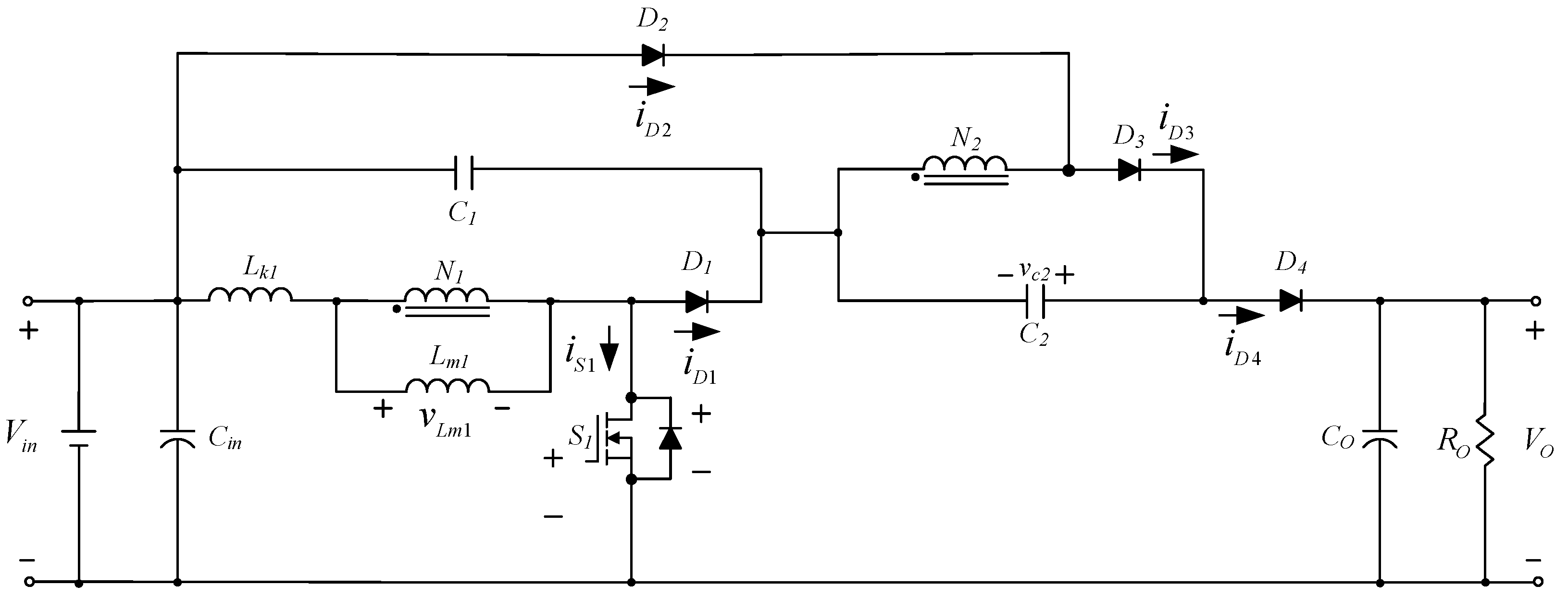
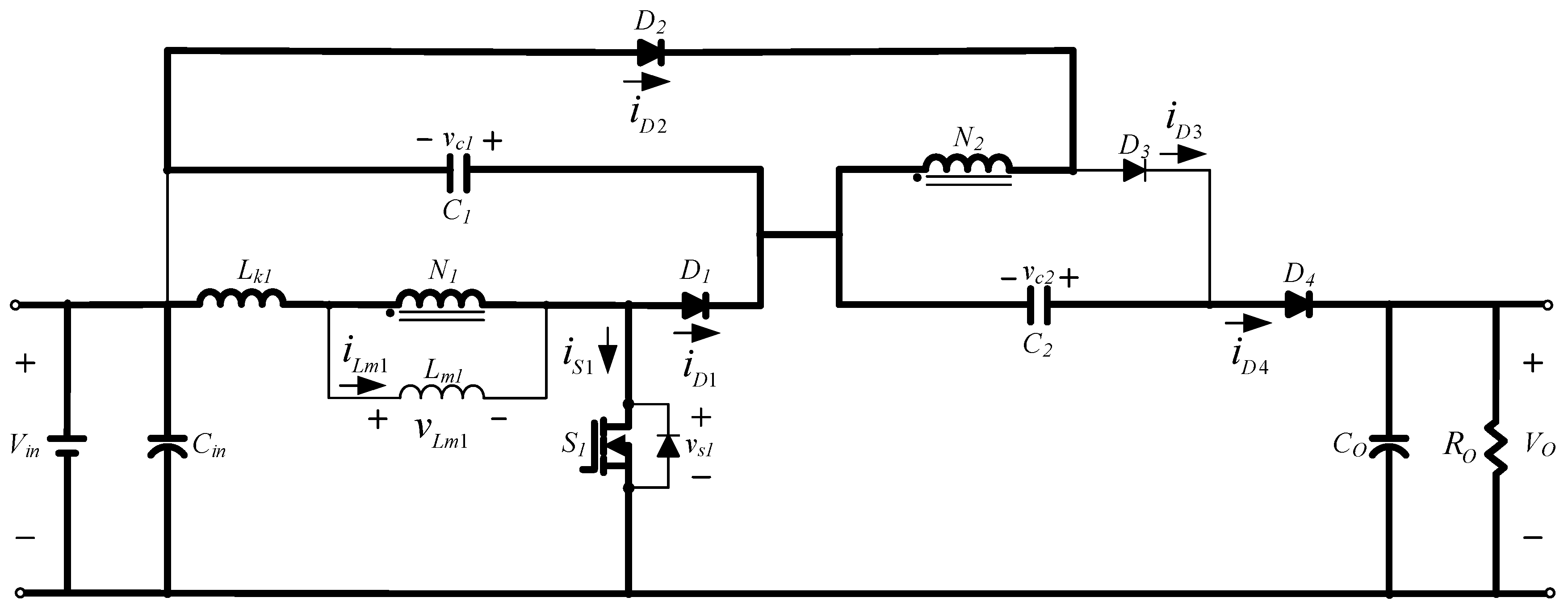
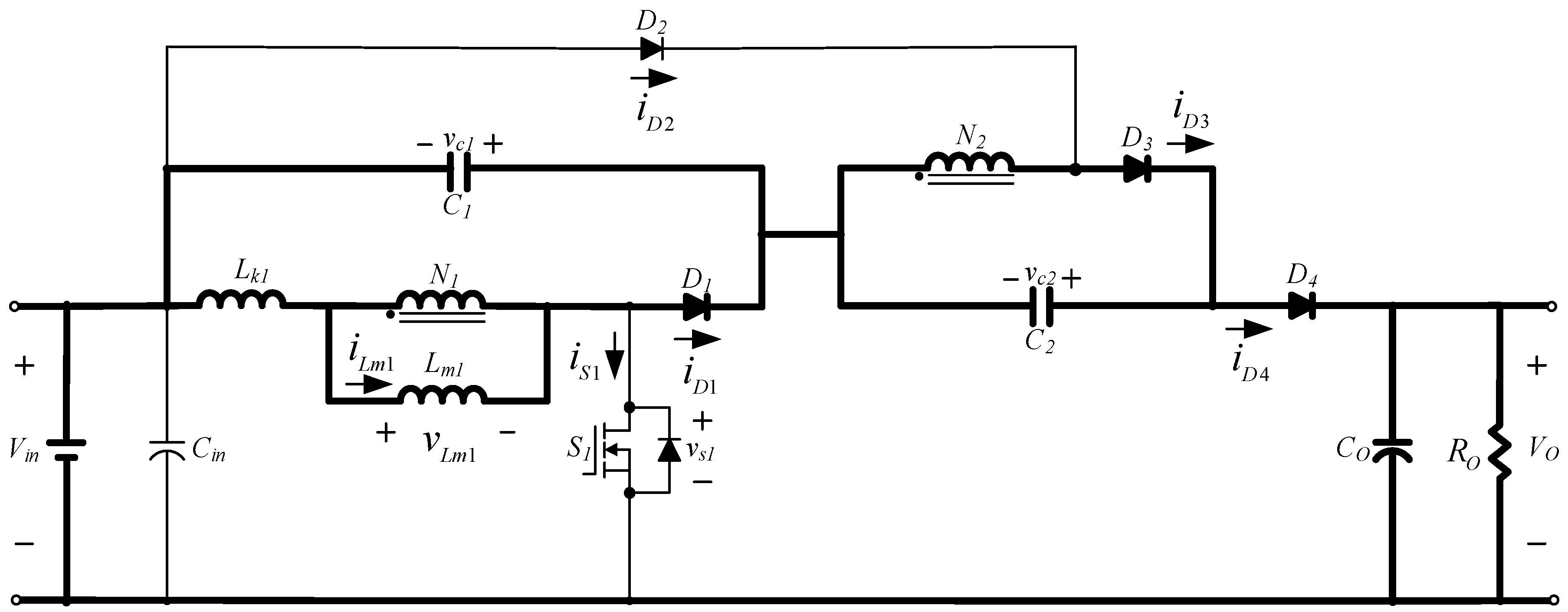
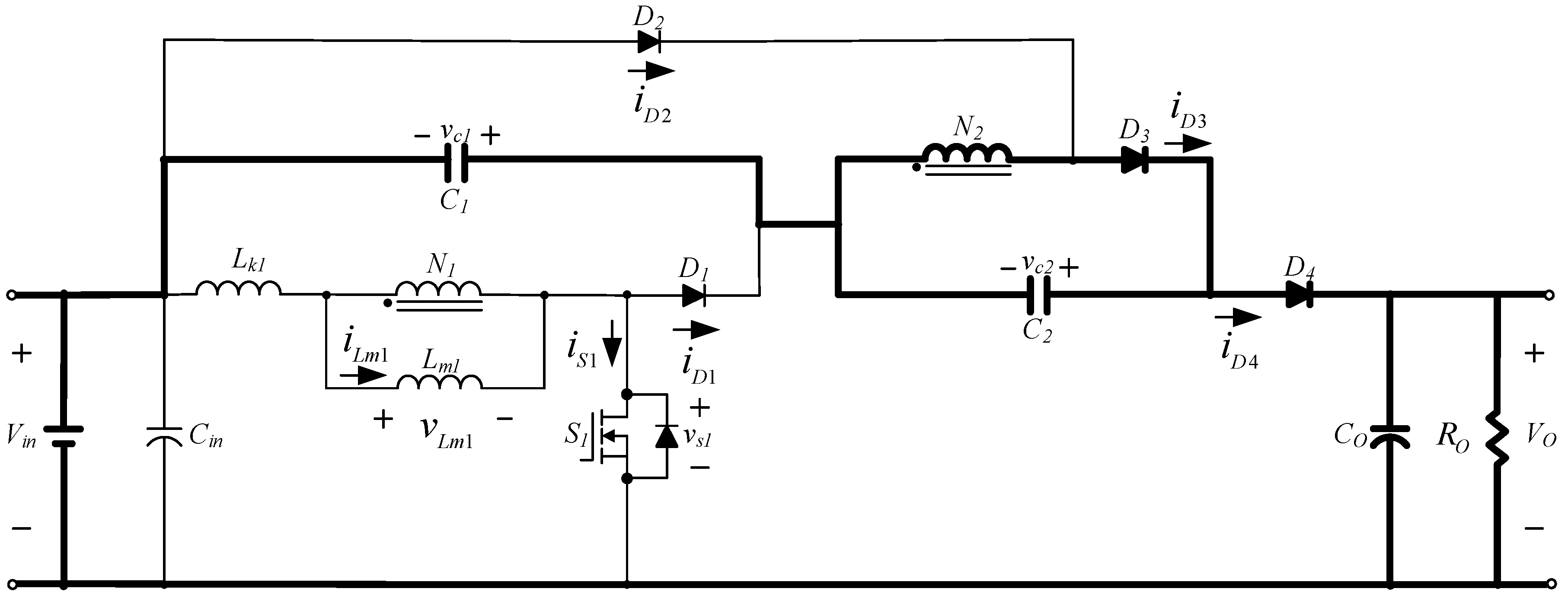
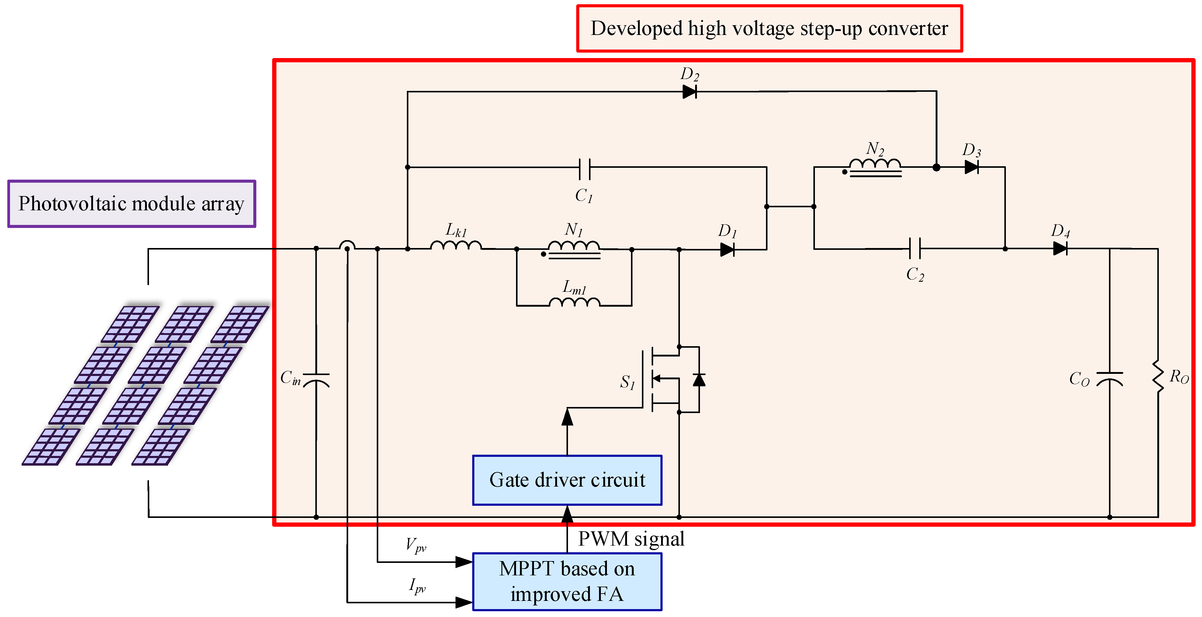
2. High Voltage Boost Converter
- (1)
- Mode 1 ()
- (2)
- Mode 2 ()
- (3)
- Mode 3 ()
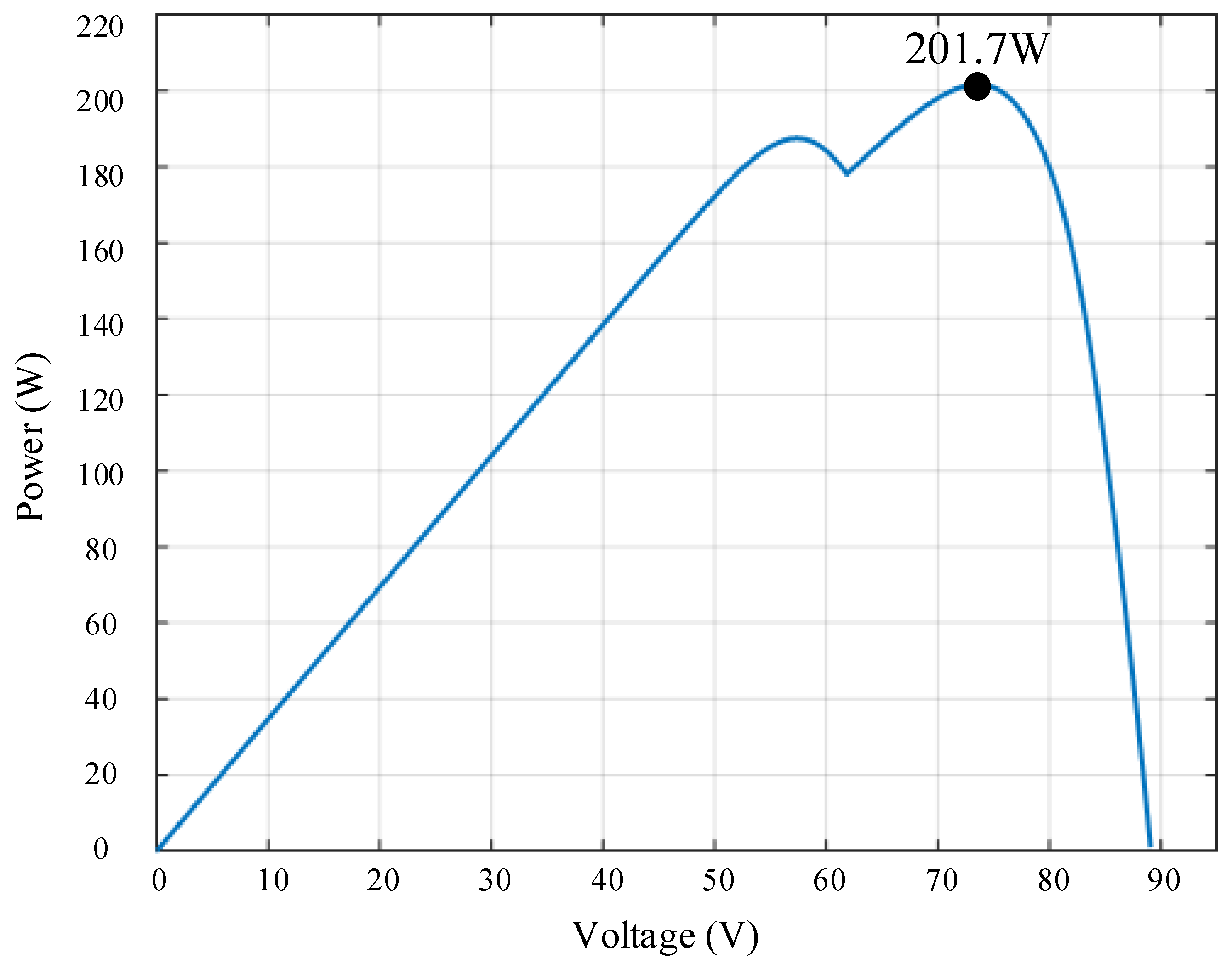
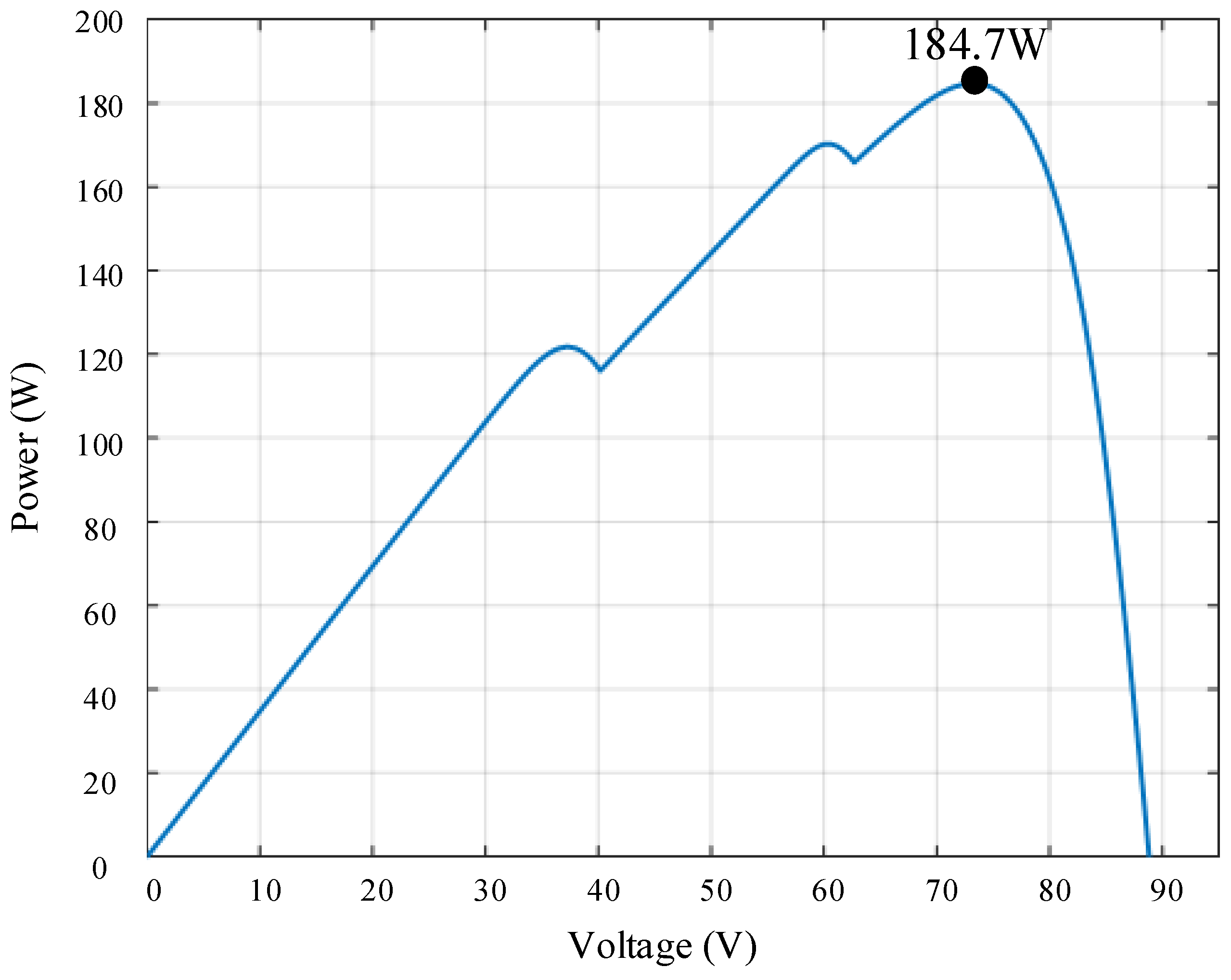
3. Shading Dependence of Output Characteristics of a PV Array
4. Firefly Algorithms
4.1. The Conventional FA
- (1)
- Fireflies are attracted to each other despite their gender.
- (2)
- Level of attraction is simply a function of the light intensity and the distance between fireflies, and it decreases as the distance increases. Fireflies which glow with lower brightness are attracted to those with higher brightness—which move randomly.
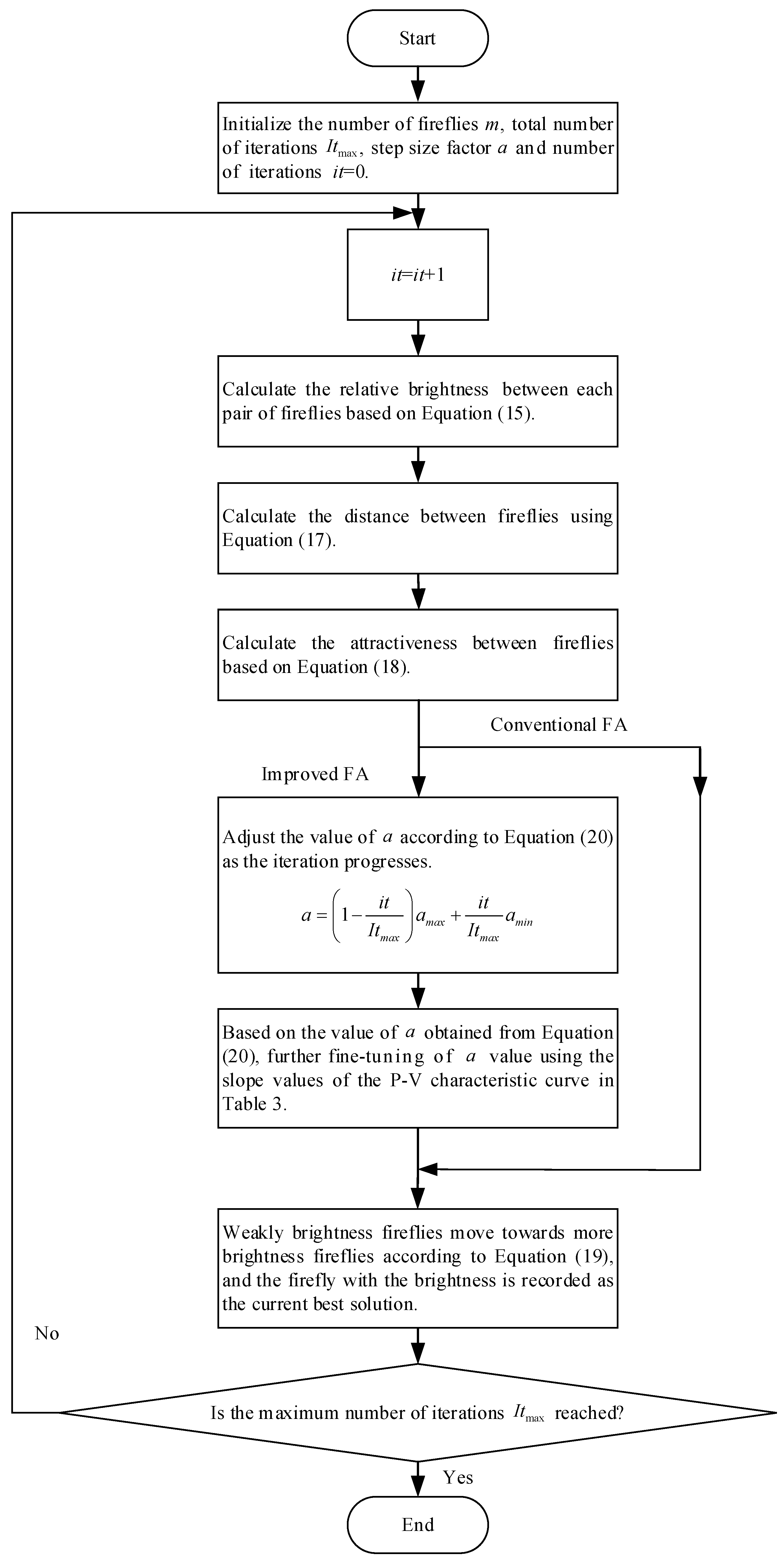
- Step 1:
- Initialize the number of fireflies , the maximum number of iterations and the step size .
- Step 2:
- The relative brightness between a firefly and another is given bywhere represents the brightness emitted by the firefly, and the absorption coefficient of a medium. decays as the distance increases, and is usually considered a constant.
- Step 3:
- In an n-dimensional space, the distance between fireflies i and j is expressed aswhere represents the n coordinate of firefly j. In this work, the FA is applied to track the MPP of a PV array, and the n-dimensional space is therefore simplified to a plane. Hence, Equation (16) becomes
- Step 4:
- Level of attraction is given bywhere represents the maximum of .
- Step 5:
- Firefly i is attracted to firefly j, and the position of firefly i is updated usingwhere r is a random number between 0 and 1.
- Step 6:
- Go back to Step 1 until the maximum number of iterations is reached, and then output .
4.2. The Improved FA
5. Simulation Results
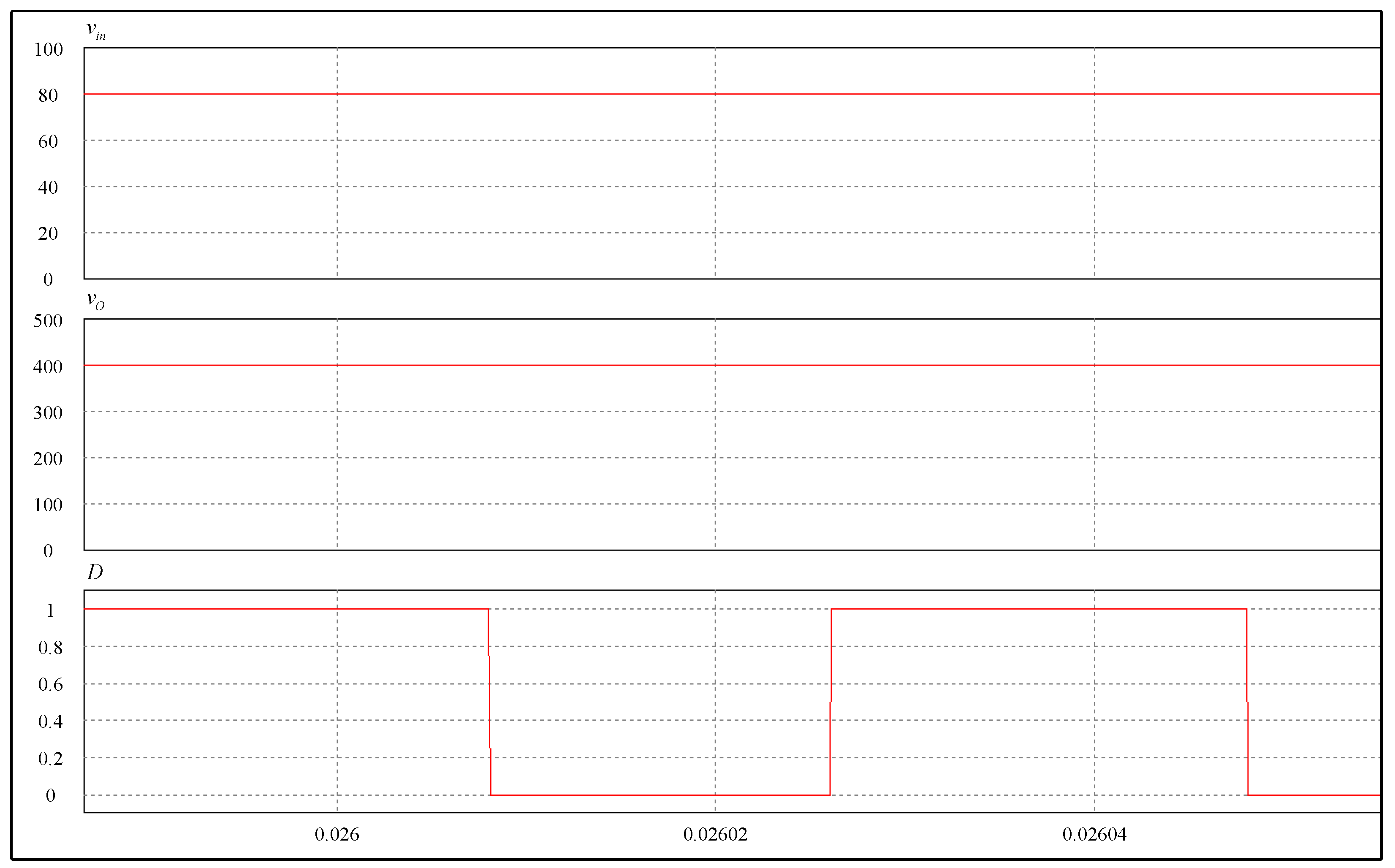
5.1. Simulation Results of the Proposed Converter
5.2. Simulation Results of the Improved FA
- (1)
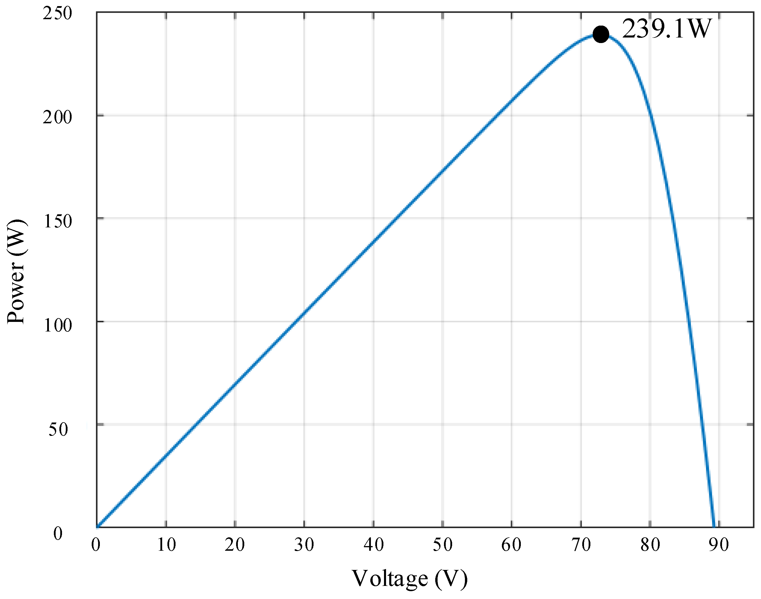
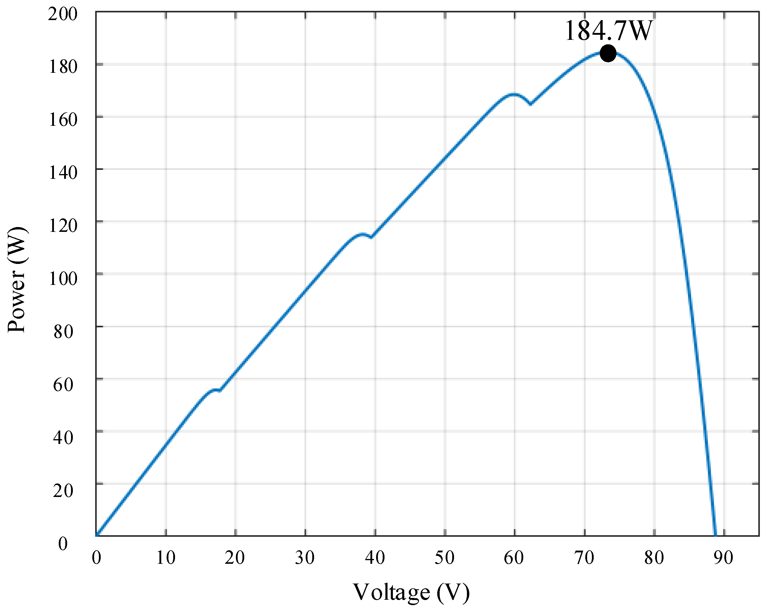
- Scenario 1
- (2)
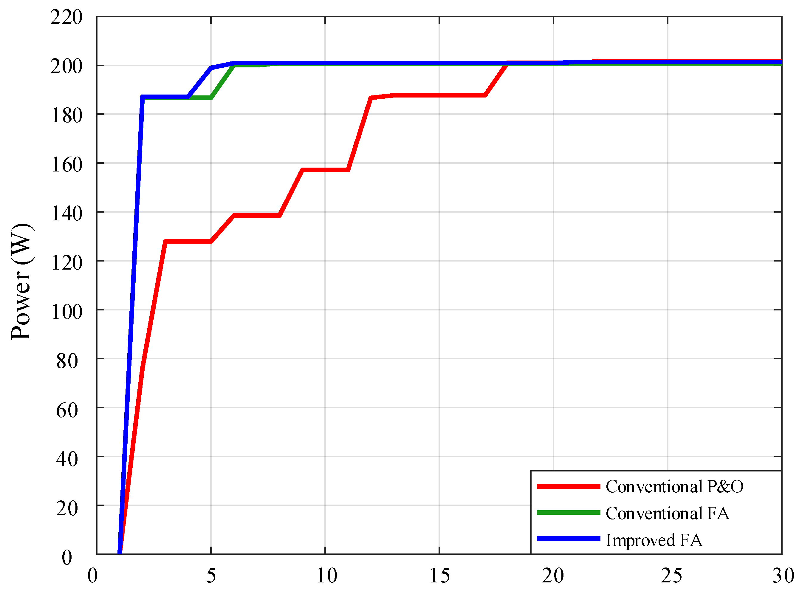
- Scenario 2
- (3)
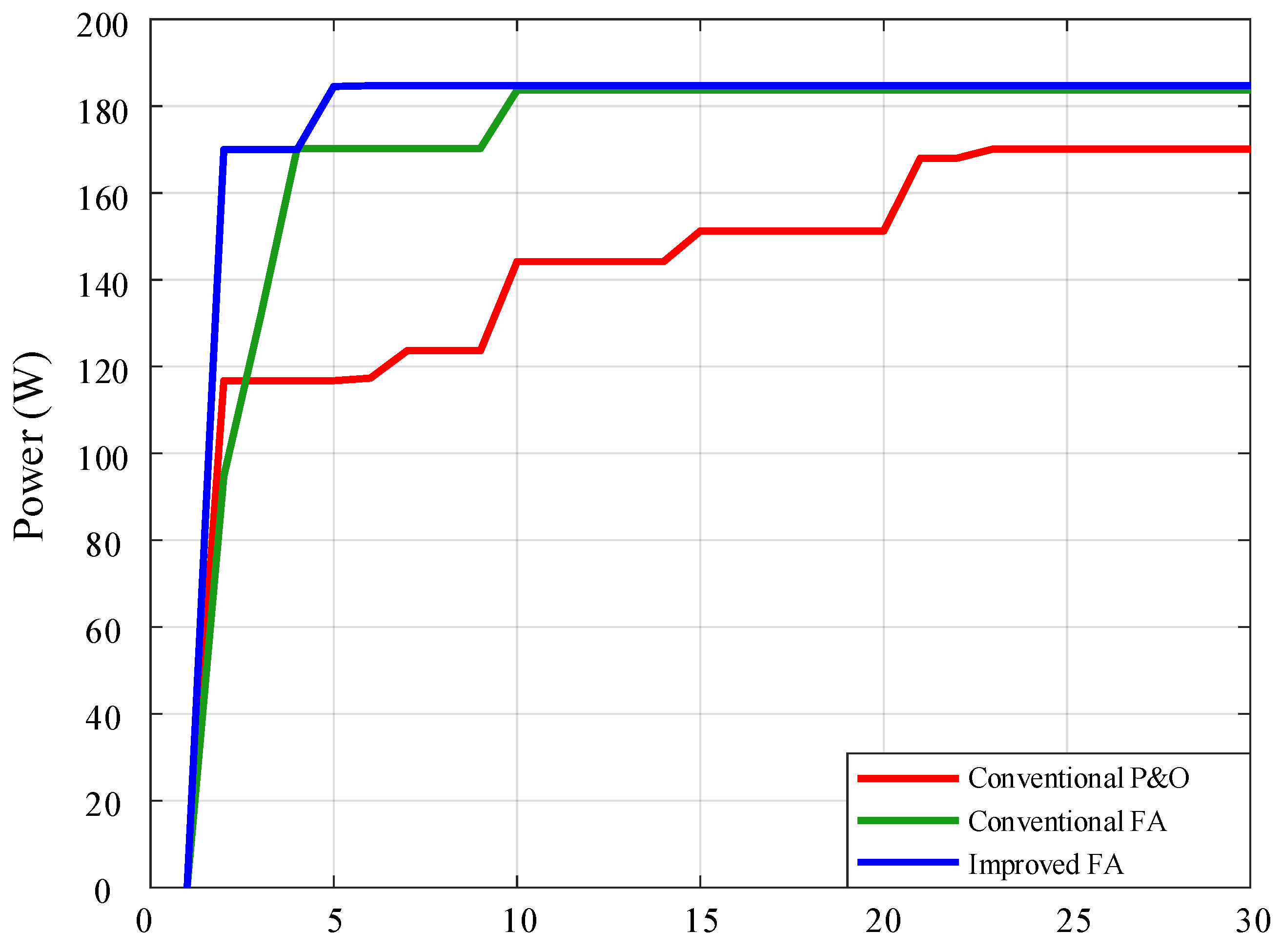
- Scenario 3
- (4)
- Scenario 4
- (5)
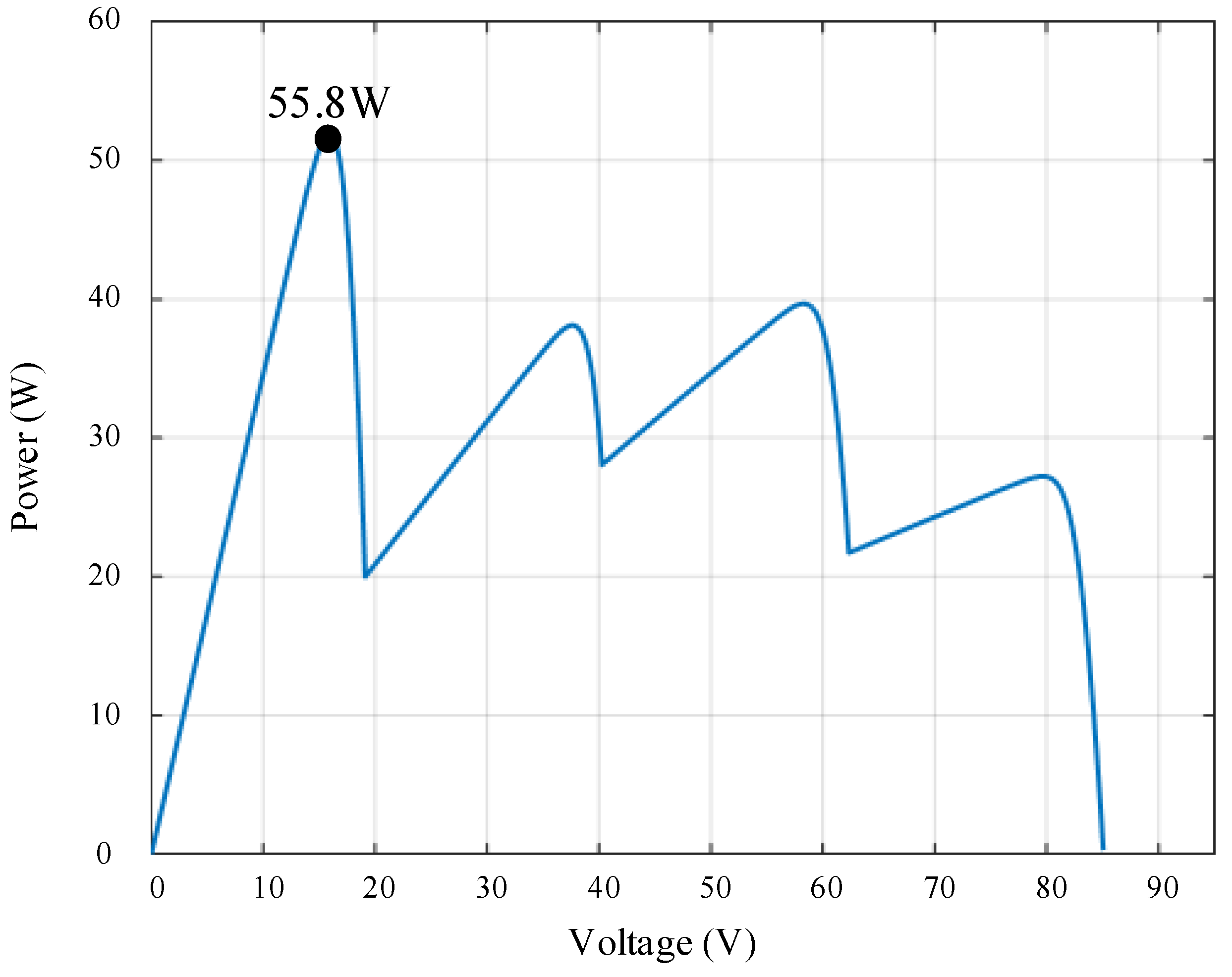
- Scenario 5
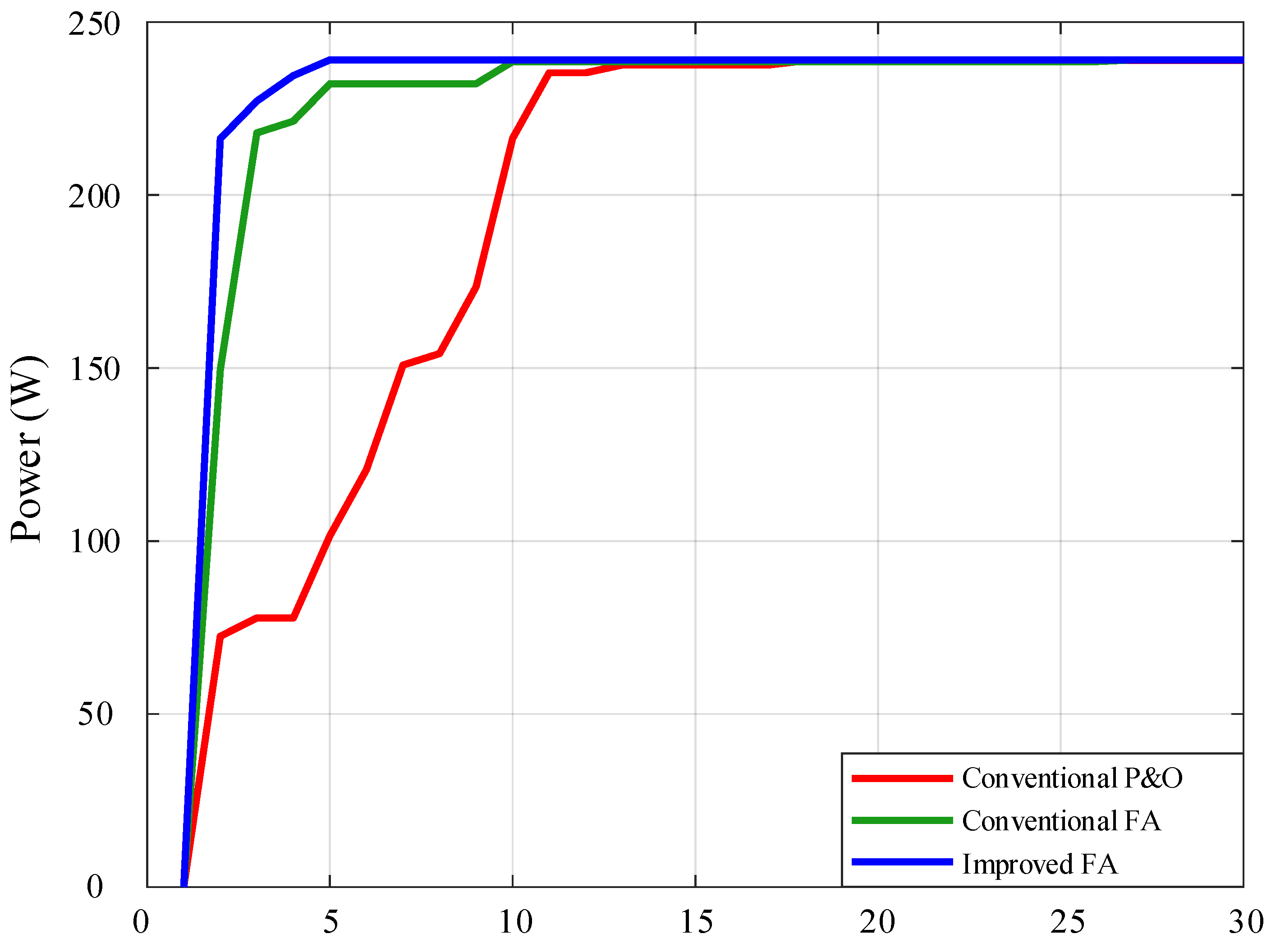
5.3. Discussion of the Simulation Results
6. Conclusions
Author Contributions
Funding
Institutional Review Board Statement
Informed Consent Statement
Data Availability Statement
Conflicts of Interest
References
- Wei, Q.; Shi, G.; Song, R.; Liu, Y. Adaptive Dynamic Programming-based Optimal Control Scheme for Energy Storage Systems with Solar Renewable Energy. IEEE Trans. Ind. Electron. 2017, 64, 5468–5478. [Google Scholar] [CrossRef]
- Safdarian, A.; Fotuhi-Firuzabad, M.; Aminifar, F. Compromising Wind and Solar Energies from the Power System Adequacy Viewpoint. IEEE Trans. Power Syst. 2012, 27, 2368–2376. [Google Scholar] [CrossRef]
- Jones, D.C.; Erickson, R.W. Probabilistic Analysis of a Generalized Perturb and Observe Algorithm Featuring Robust Operation in the Presence of Power Curve Traps. IEEE Trans. Power Electron. 2013, 28, 2912–2926. [Google Scholar] [CrossRef]
- Killi, M.; Samanta, S. Modified Perturb and Observe MPPT Algorithm for Drift Avoidance in Photovoltaic Systems. IEEE Trans. Ind. Electron. 2015, 62, 5549–5559. [Google Scholar] [CrossRef]
- Sher, H.A.; Murtaza, A.F.; Noman, A.; Addoweesh, K.E.; Al-Haddad, K.; Chiaberge, M. A New Sensorless Hybrid MPPT Algorithm Based on Fractional Short-circuit Current Measurement and P&O MPPT. IEEE Trans. Sust. Energy 2015, 6, 1426–1434. [Google Scholar]
- Sahu, R.K.; Ghosh, A. Maximum Power Generation from Solar Panel by Using P&O MPPT. In Proceedings of the International Conference on Intelligent Controller and Computing for Smart Power (ICICCSP), Hyderabad, India, 21–23 July 2022; pp. 1–4. [Google Scholar]
- Utaikaifa, K. Reduction of Power Ripple in P&O MPPT System Using Output Feedback. In Proceedings of the 4th International Conference on Power Engineering, Energy and Electrical Drives, Istanbul, Turkey, 13–17 May 2013; pp. 427–432. [Google Scholar]
- Szemes, P.T.; Melhem, M. Analyzing and Modeling PV with “P&O” MPPT Algorithm by MATLAB/SIMULINK. In Proceedings of the 3rd International Symposium on Small-Scale Intelligent Manufacturing Systems (SIMS), Gjovik, Norway, 10–12 June 2020; pp. 1–6. [Google Scholar]
- Liu, F.; Duan, S.; Liu, F.; Liu, B.; Kang, Y. A Variable Step Size INC MPPT Method for PV Systems. IEEE Trans. Ind. Electron. 2008, 55, 2622–2628. [Google Scholar]
- Bhattacharyya, S.; Kumar, D.S.; Samanta, S.; Mishra, S. Steady Output and Fast Tracking MPPT (SOFT-MPPT) for P&O and INC Algorithms. IEEE Trans. Sust. Energy 2021, 12, 293–302. [Google Scholar]
- Saber, H.; Bendaouad, A.E.; Rahmani, L.; Radjeai, H. A Comparative Study of the FLC, INC and P&O Methods of the MPPT Algorithm for a PV System. In Proceedings of the 19th International Multi-Conference on Systems, Signals & Devices (SSD), Sétif, Algeria, 6–10 May 2022; pp. 2010–2015. [Google Scholar]
- Zhang, H.; Li, S.Z.; Zhang, X.N.; Xia, Y.L. MPPT Control Strategy for Photovoltaic Cells Based on Fuzzy Control. In Proceedings of the 12th International Conference on Natural Computation, Fuzzy Systems and Knowledge Discovery (ICNC-FSKD), Changsha, China, 13–15 August 2016; pp. 450–454. [Google Scholar]
- Subasic, P.; Nakatsuyama, M. A New Representational Framework for Fuzzy Sets. In Proceedings of the 6th International Fuzzy Systems Conference, Barcelona, Spain, 5 July 1997; pp. 1601–1606. [Google Scholar]
- Rai, R.K.; Rahi, O.P. Fuzzy Logic based Control Technique Using MPPT for Solar PV System. In Proceedings of the First International Conference on Electrical, Electronics, Information and Communication Technologies (ICEEICT), Trichy, India, 16–18 February 2022; pp. 1–5. [Google Scholar]
- Prokhorov, D. Echo State Networks: Appeal and Challenges. In Proceedings of the IEEE International Joint Conference on Neural Networks, Montreal, QC, Canada, 31 July–4 August 2005; pp. 1463–1466. [Google Scholar]
- Dahidi, S.A.; Ayadi, O.; Alrbai, M.; Adeeb, J. Ensemble Approach of Optimized Artificial Neural Networks for Solar Photovoltaic Power Prediction. IEEE Access 2019, 7, 81741–81758. [Google Scholar] [CrossRef]
- Shukla, A.; Titare, L.S. An Efficient Neural Network-based MPPT Technique for PV Array under Partial Shading Conditions. In Proceedings of the International Conference on Smart Generation Computing, Communication and Networking (SMART GENCON), Pune, India, 29–30 October 2021; pp. 1–5. [Google Scholar]
- Mohanty, S.; Subudhi, B.; Ray, P.K. A Grey Wolf Optimization Based MPPT for PV System under Changing Insolation Level. In Proceedings of the IEEE Students’ Technology Symposium (TechSym), Kharagpur, India, 30 September–2 October 2016; pp. 175–179. [Google Scholar]
- Atici, K.; Sefa, I.; Altin, N. Grey Wolf Optimization Based MPPT Algorithm for Solar PV System with SEPIC Converter. In Proceedings of the 4th International Conference on Power Electronics and their Applications (ICPEA), Elazig, Turkey, 25–27 September 2019; pp. 1–6. [Google Scholar]
- Hasan, F.R.; Prasetyono, E.; Sunarno, E. A Modified Maximum Power Point Tracking Algorithm Using Grey Wolf Optimization for Constant Power Generation of Photovoltaic System. In Proceedings of the International Conference on Artificial Intelligence and Mechatronics Systems (AIMS), Bandung, Indonesia, 28–30 April 2021; pp. 1–6. [Google Scholar]
- Firmanza, A.P.; Habibi, M.N.; Windarko, N.A.; Yanaratri, D.S. Differential Evolution-based MPPT with Dual Mutation for PV Array under Partial Shading Condition. In Proceedings of the 10th Electrical Power, Electronics, Communications, Controls and Informatics Seminar (EECCIS), Malang, Indonesia, 26–28 August 2020; pp. 198–203. [Google Scholar]
- Tajuddin, M.F.N.; Ayob, S.M.; Salam, Z. Tracking of Maximum Power Point in Partial Shading Condition Using Differential Evolution (DE). In Proceedings of the IEEE International Conference on Power and Energy (PECon), Kota Kinabalu, Malaysia, 2–5 December 2012; pp. 384–389. [Google Scholar]
- Taheri, H.; Salam, Z.; Ishaque, K. Syafaruddin A Novel Maximum Power Point Tracking Control of Photovoltaic System under Partial and Rapidly Fluctuating Shadow Conditions Using Differential Evolution. In Proceedings of the IEEE Symposium on Industrial Electronics and Applications (ISIEA), Penang, Malaysia, 3–5 October 2010; pp. 82–87. [Google Scholar]
- Castano, C.G.; Restrepo, C.; Kouro, S.; Rodriguez, J. MPPT Algorithm Based on Artificial Bee Colony for PV System. IEEE Access 2021, 9, 43121–43133. [Google Scholar] [CrossRef]
- Li, N.; Mingxuan, M.; Yihao, W.; Lichuang, C.; Lin, Z.; Qianjin, Z. Maximum Power Point Tracking Control Based on Modified ABC Algorithm for Shaded PV System. In Proceedings of the International Conference of Electrical and Electronic Technologies for Automotive (AEIT AUTOMOTIVE), Turin, Italy, 2–4 July 2019; pp. 1–5. [Google Scholar]
- Pilakkat, D.; Kanthalakshmi, S. Artificial Bee Colony Algorithm for Peak Power Point Tracking of a Photovoltaic System under Partial Shading Condition. In Proceedings of the International Conference on Current Trends towards Converging Technologies (ICCTCT), Coimbatore, India, 1–3 March 2018; pp. 1–7. [Google Scholar]
- Huang, Y.P.; Huang, M.Y.; Ye, C.E. A Fusion Firefly Algorithm with Simplified Propagation for Photovoltaic MPPT under Partial Shading Conditions. IEEE Trans. Sust. Energy 2020, 11, 2641–2652. [Google Scholar] [CrossRef]
- Teshome, D.F.; Lee, C.H.; Lin, Y.W.; Lian, K.L. A Modified Firefly Algorithm for Photovoltaic Maximum Power Point Tracking Control under Partial Shading. IEEE J. Emerg. Sel. Topics Power Electron. 2016, 5, 661–671. [Google Scholar] [CrossRef]
- Windarko, N.A.; Tjahjono, A.; Anggriawan, D.O.; Purnomo, M.H. Maximum Power Point Tracking of Photovoltaic System Using Adaptive Modified Firefly Algorithm. In Proceedings of the International Electronics Symposium (IES), Surabaya, Indonesia, 29–30 September 2015; pp. 31–35. [Google Scholar]
- Li, C.C.; Sun, C.Y.; Li, S.Q.; Zhang, Y.Y. An Integrated MPPT Control Strategy Using Circle Search-firefly Algorithm (CSFA) for Photovoltaic System. In Proceedings of the 4th International Conference on Smart Power & Internet Energy Systems (SPIES), Beijing, China, 9–12 December 2022; pp. 1945–1949. [Google Scholar]
- Mohammad, M.; Rabeh, A.; Houssem, J.; Faraedoon, W.A.; Halkawt, A.; Alireza, R. A New MPPT Design Using Variable Step Size Perturb and Observe Method for PV System under Partially Shaded Conditions by Modified Shuffled Frog Leaping Algorithm-SMC Controller. Sustain. Energy Technol. Assess. 2021, 45, 101056. [Google Scholar]
- Guo, S.; Abbassi, R.; Jerbi, H.; Rezvani, A.; Suzuki, K. Efficient Maximum Power Point Tracking for a Photovoltaic Using Hybrid Shuffled Frog-leaping and Pattern Search Algorithm under Changing Environmental Conditions. J. Clean. Prod. 2021, 297, 126573. [Google Scholar] [CrossRef]
- Tian, H.; Bai, Q.; Li, X.; Han, H.; Maoa, S.; Yang, H.; Wang, H. Comparative Study on Fill Factor of PERC Silicon Solar Cells and Al-BSF Silicon Solar Cells under Non-standard Test Conditions. In Proceedings of the IEEE 48th Photovoltaic Specialists Conference (PVSC)s, Fort Lauderdale, FL, USA, 20–25 June 2021; pp. 256–259. [Google Scholar]
- Forouzesh, M.; Siwakoti, Y.P.; Gorji, S.A.; Blaabjerg, F.; Lehman, B. Step-up DC–DC Converters: A Comprehensive Review of Voltage-boosting Techniques, Topologies, and Applications. IEEE Trans. Power Electron. 2017, 32, 9143–9178. [Google Scholar] [CrossRef]
- Park, D.; Lee, H. Improvements in Light-load Efficiency and Operation Frequency for Low-voltage Current-mode Integrated Boost Converters. IEEE Trans. Circuits Syst. II Express Briefs 2014, 61, 599–603. [Google Scholar] [CrossRef]
- Park, K.B.; Moon, G.W.; Youn, M.J. Overview of High-step-up Coupled-inductor Boost Converters. IEEE J. Emerg. Sel. Topics Power Electron. 2016, 4, 689–704. [Google Scholar]
- Park, K.B.; Moon, G.W.; Youn, M.J. Nonisolated High Step-up Stacked Converter Based on Boost-integrated Isolated Converter. IEEE Trans. Power Electron. 2011, 26, 577–587. [Google Scholar] [CrossRef]
- Schmitz, L.; Martins, D.C.; Coelho, R.F. Generalized High Step-up DC-DC Boost-based Converter with Gain Cell. IEEE Trans. Circuits Syst. I: Regular Papers 2017, 64, 480–493. [Google Scholar] [CrossRef]
- Park, K.B.; Moon, G.W.; Youn, M.J. Nonisolated High Step-up Boost Converter Integrated with Sepic Converter. IEEE Trans. Power Electron. 2010, 25, 2266–2275. [Google Scholar] [CrossRef]
- Park, K.B.; Moon, G.W.; Youn, M.J. High Step-up Boost Converter Integrated with a Transformer-assisted Auxiliary Circuit Employing Quasi-resonant Operation. IEEE Trans. Power Electron. 2012, 27, 1974–1984. [Google Scholar] [CrossRef]
- PSIM-User-Manual.pdf, Powersim. Available online: https://powersimtech.com/wp-content/uploads/2021/01/PSIM-User-Manual.pdf (accessed on 21 February 2023).
- Chao, K.H.; Zhang, S.W. An Maximum Power Point Tracker of Photovoltaic Module Arrays Based on Improved Firefly Algorithm. Sustainability 2023, 15, 8550. [Google Scholar] [CrossRef]
- Khan, R.; Khan, L.; Ullah, S.; Sami, I.; Ro, J.S. Backstepping Based Super-Twisting Sliding Mode MPPT Control with Differential Flatness Oriented Observer Design for Photovoltaic System. J. Power Electron. 2020, 9, 1543. [Google Scholar] [CrossRef]
- Ali, K.; Khan, L.; Khan, Q.; Ullah, S.; Ahmad, S.; Mumtaz, S.; Karam, F.W.; Naghmash. Robust Integral Backstepping Based Nonlinear MPPT Control for a PV System. Energies 2019, 12, 3180. [Google Scholar] [CrossRef] [Green Version]


| Input voltage () | 80 V |
| Output voltage () | 400 V |
| Output power () | 300 W |
| Switching frequency of power switch (f) | 25 kHz |
| Turn ratio of inductor () | 2 |
| Parameter | Specification |
|---|---|
| Maximum output power () | 20 W |
| Current of MPP () | 1.10 A |
| Voltage of MPP () | 18.18 V |
| Short current () | 1.15 A |
| Open voltage () | 22.32 V |
| Size of module | 395 × 345 × 17 mm |
| Fine-Tuningof Equation (20) | |
| of Equation (20) + s 0.01 | |
| of Equation (20) + s 0.01 | |
| of Equation (20) − s 0.01 | |
| of Equation (20) − s 0.03 | |
| of Equation (20) − s 0.04 | |
| of Equation (20) + s 0.04 | |
| of Equation (20) + s 0.03 | |
| of Equation (20) + s 0.01 | |
| of Equation (20) − s 0.01 | |
| of Equation (20) − s 0.01 |
| Parameter Name | Value |
|---|---|
| Number of fireflies () | 4 |
| Maximum number of iterations () | 30 |
| Step size () | 2 |
| Parameter Name | Value |
|---|---|
| Number of fireflies () | 4 |
| Maximum number of iterations () | 30 |
| Upper bound of step size () | 2.5 |
| Lower bound of step size () | 1.5 |
| Scenario | Module Connection and Shading Condition | Number of P-V Curve Peaks |
|---|---|---|
| 1 | (0% shading + 0% shading + 0% shading +0% shading)// (0% shading + 0% shading + 0% shading + 0% shading)// (0% shading + 0% shading + 0% shading +0% shading) | Single |
| 2 | (0% shading + 0% shading + 0% shading + 50% shading)// (0% shading + 0% shading + 0% shading + 0% shading)// (0% shading + 0% shading + 0% shading + 0% shading) | Double (MPP was on the rightmost peak) |
| 3 | (0% shading + 0% shading + 50% shading + 70%shading)// (0% shading + 0% shading + 0% shading + 0% shading)// (0% shading + 0% shading + 0% shading + 0% shading) | Triple (MPP was on the rightmost peak) |
| 4 | (0% shading + 30% shading + 50% shading + 70% shading)// (0% shading + 0% shading + 0% shading + 0% shading)// (0% shading + 0% shading + 0% shading + 0% shading) | Triple (MPP was on the rightmost peak) |
| 5 | (0% shading + 70% shading + 80% shading + 90% shading)// (0% shading + 70% shading + 80% shading + 90% shading)// (0% shading + 70% shading + 80% shading + 90% shading) | Quadruple (MPP was on the leftmost peak) |
| Scenario | No. of Peaks on Respective P-V Curve | Average Number of Iterations/Average Tracking Time | ||
|---|---|---|---|---|
| Conventional P&O | Conventional FA | Improved FA | ||
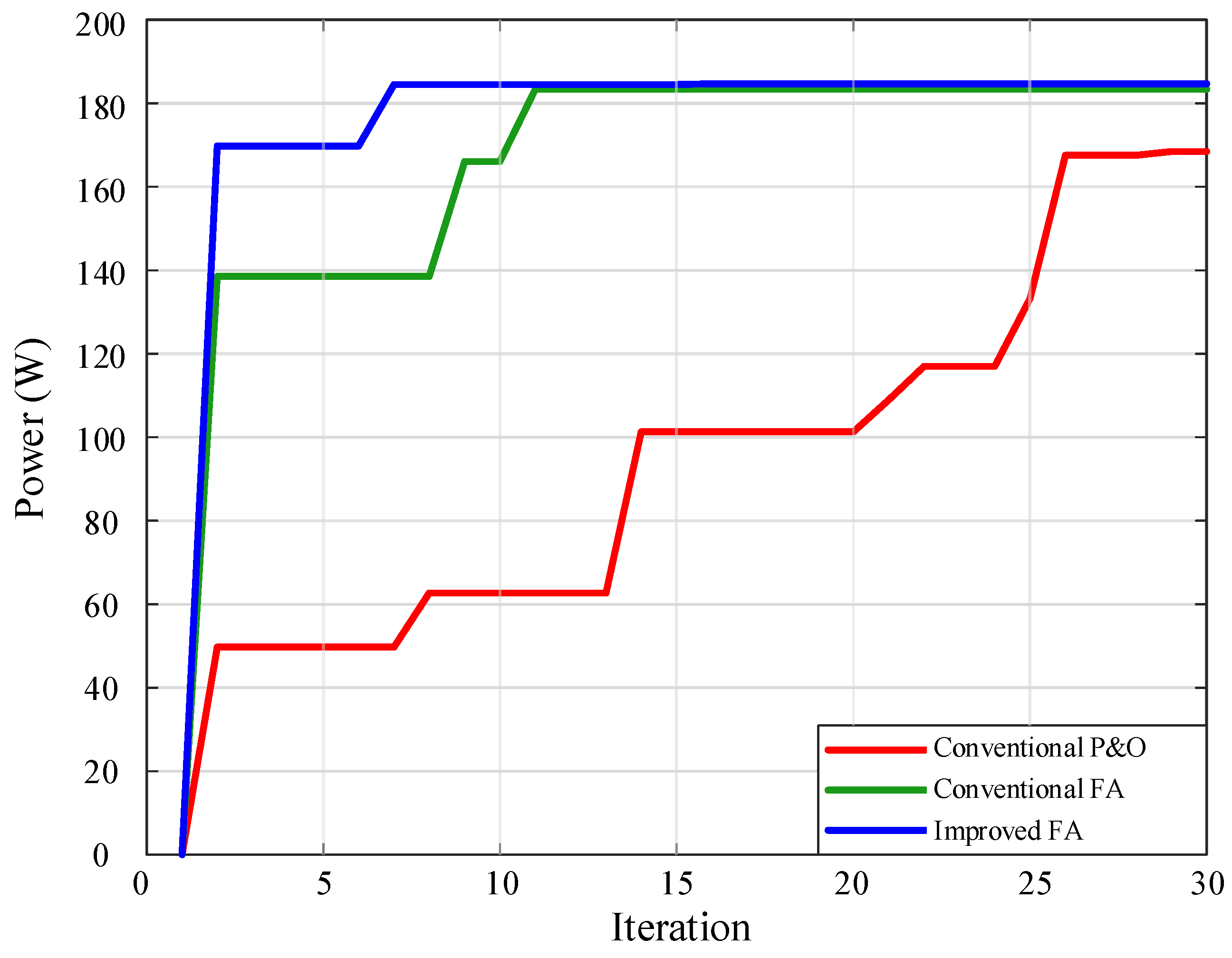
| 1 | Single | 10.4/5.2 s | 5.6/2.8 s | 3.4/0.7 s |
| 2 | Double (MPP was on the right peak) | 19.5/7.6 s | 8.4/3.4 s | 5.7/0.9 s |
| 3 | Triple (MPP was on the rightmost peak) | not available | 14.1/4.0 s | 12.7/1.3 s |
| 4 | Quadruple (MPP was on the rightmost peak) | not available | 14.3/4.2 s | 12.8/1.6 s |
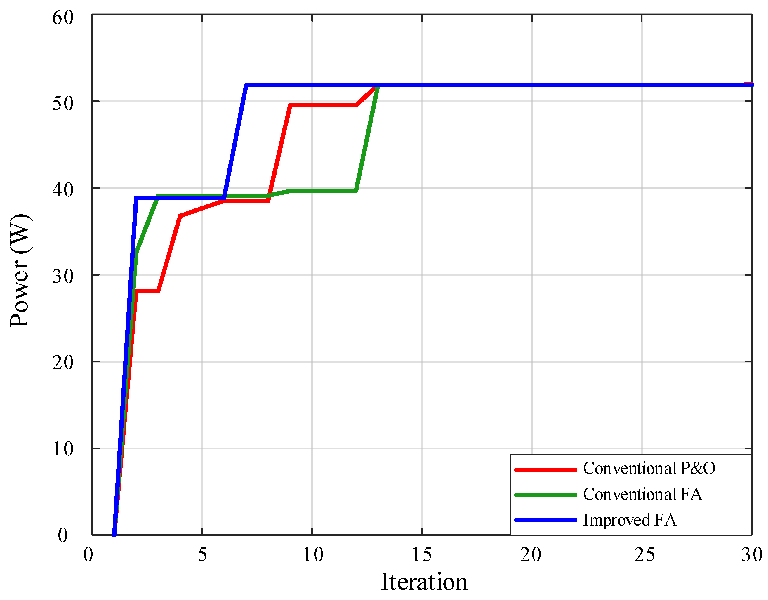
| 5 | Quadruple (MPP was on the leftmost peak) | 22.8/5.8 s | 17.2/4.7 s | 14.1/2.0 s |
| Scenario | No. Peak(s) of the P-V Curve | Method Proposed in [3] | Method Proposed in [18] | Method Proposed in [24] | Proposed in this Study |
|---|---|---|---|---|---|
| Average Tracking Time | Average Tracking Time | Average Tracking Time | Average Tracking Time | ||
| 1 | Single-peak | 10.4 s | 8.6 s | 8.58 s | 3.4 s |
| 2 | Double-peak | 19.5 s | 12.5 s | 20.01 s | 5.7 s |
| 3 | Triple-peak | None * | 15.4 s | 31.3 s | 12.7 s |
| 4 | Quadruple-peak | None * | 20.8 s | 24.21 s | 12.8 s |
| Scenario | No. of Peaks on Respective P-V Curve | Tracking Efficiency (%) | ||
|---|---|---|---|---|
| Conventional P&O | Conventional FA | Improved FA | ||
| 1 | Single | 78.83% | 98.32% | 99.29% |
| 2 | Double (MPP was on the right peak) | 79.25% | 98.73% | 99.09% |
| 3 | Triple (MPP was on the rightmost peak) | 67.88% | 93.23% | 98.01% |
| 4 | Quadruple (MPP was on the rightmost peak) | 42.48% | 82.96% | 96.74% |
| 5 | Quadruple (MPP was on the leftmost peak) | 77.99% | 76.1% | 89.76% |
Disclaimer/Publisher’s Note: The statements, opinions and data contained in all publications are solely those of the individual author(s) and contributor(s) and not of MDPI and/or the editor(s). MDPI and/or the editor(s) disclaim responsibility for any injury to people or property resulting from any ideas, methods, instructions or products referred to in the content. |
© 2023 by the authors. Licensee MDPI, Basel, Switzerland. This article is an open access article distributed under the terms and conditions of the Creative Commons Attribution (CC BY) license (https://creativecommons.org/licenses/by/4.0/).
Share and Cite
Chao, K.-H.; Zhang, S.-W. An Adaptive Maximum Power Point Tracker for Photovoltaic Arrays Using an Improved Soft Computing Algorithm. Appl. Sci. 2023, 13, 6952. https://doi.org/10.3390/app13126952
Chao K-H, Zhang S-W. An Adaptive Maximum Power Point Tracker for Photovoltaic Arrays Using an Improved Soft Computing Algorithm. Applied Sciences. 2023; 13(12):6952. https://doi.org/10.3390/app13126952
Chicago/Turabian StyleChao, Kuei-Hsiang, and Shu-Wei Zhang. 2023. "An Adaptive Maximum Power Point Tracker for Photovoltaic Arrays Using an Improved Soft Computing Algorithm" Applied Sciences 13, no. 12: 6952. https://doi.org/10.3390/app13126952