Article

Optimizing BiLSTM Network Attack Prediction Based on Improved Gray Wolf Algorithm

Communication and Network Laboratory, Dalian University, Dalian 116622, China
*
Author to whom correspondence should be addressed.
Appl. Sci. 2023, 13(12), 6871; https://doi.org/10.3390/app13126871
Submission received: 12 May 2023 / Revised: 1 June 2023 / Accepted: 5 June 2023 / Published: 6 June 2023
(This article belongs to the Special Issue Recent Advances in Cybersecurity and Computer Networks)

Abstract

:
Aiming at the problems of low accuracy of network attack prediction and long response time of attack detection, bidirectional long short-term memory (BiLSTM) was used to predict network attacks. However, BiLSTM has the problems of difficulty in parameter setting and low accuracy of the prediction model. This paper first proposes the Improved Grey Wolf algorithm (IGWO) to optimize the BiLSTM (IGWO-BiLSTM). First, IGWO uses Dimension Learning Hunting (DLH) strategy to construct the wolf neighborhood. In the established wolf neighborhood, the BiLSTM parameters are iteratively optimized to obtain a prediction model with fast convergence speed and small reconstruction error. Secondly, the dataset is preprocessed, and the IP packet statistical signature (IPDCF) is defined according to the characteristics of denial of service (DOS) and distributed denial of service (DDOS) attacks. IPDCF was used to establish the time series model and network traffic time series data were input into IGWO-BiLSTM to get the prediction results. Finally, the DOS and DDOS network packets were input into the trained prediction model to obtain the prediction results of attack data. By comparing the predicted values of IGWO-BiLSTM normal network packets and attack packets, a reasonable threshold is set to provide the basis for the subsequent attack prediction. Experiments show that the IGWO-BiLSTM can reach 99.05% of the fitting degree and accurately distinguish network attacks from normal network demand increases.

1. Introduction

With the development of computer technology, more and more devices are connected to the network. Therefore, network traffic is becoming more and more complex, and the network security problem has ushered in new challenges. Because of its unique abruptness, network traffic requires a high prediction model. This paper mainly studies the use of IGWO-BiLSTM to predict network attacks. In this section, we introduce motivation, related studies and contributions.

1.1. Motivation

Network security is very important because network security includes all forms of data security and information security. With the development of network information technology, incidents such as information leakage and phishing continue to occur [1], therefore, the importance of network security is increasingly recognized. The existing security protection schemes include firewalls, data encryption, intrusion detection system [2], etc. Firewalls and data encryption are passive security protection technology, which can only protect network security after a network attack occurs, while an intrusion detection system is a proactive security protection technology. Cyber-attacks provide security managers with response decisions.
Dos and DDos are based on time series and occur aperiodically. They produce and send massive amounts of useless data and network bandwidth are consumed. As a result, the attacked host cannot communicate with the outside world. Dos and DDos include many types such as user datagram protocol flood [3], acknowledge type, domain name system amplification request, etc. At present, the research on defense against DoS and DDoS mainly focuses on post-detection. However, malicious traffic is generated during attacks [4], and any measures taken at this time are limited to mitigate the damage. The industry [5] is improving its ability to defend against attacks by deploying more dynamic defense systems but costs will increase accordingly. Hence, how to accurately predict DoS and DDoS before they happen is very important.

1.2. Related Studies

Existing studies have established the time series of normal network traffic [6] and used the time series to train the prediction model. Researchers’ prediction of time series [7] can be divided into linear and nonlinear forecasts. Autoregressive (AR) is the simplest linear time series prediction model, which is suitable for predicting traffic data related to its previous period. The prediction result of AR is extremely inaccurate for traffic data greatly affected by external factors. In literature [8], AR is introduced to predict the shear stress of the fault zone. The method uses past data to predict future data to predict when an earthquake will start and end. Moving average (MA) is one of the most common ways to process time series. Autoregressive moving average (ARMA) is a combination of AR and MA used to process stationary non-white noise time series flow data. Literature [9] used a linear model to predict the monthly discharge of hydropower stations in Brazil and found that ARMA had the best performance through experiments. Autoregressive integrated moving average (ARIMA) is a combination of the ARMA model and difference operation, which can model fit stationary and non-stationary data. Literature [10], the ARIMA model was used to predict the daily number of COVID-19 cases in Saudi Arabia in the next four weeks. The linear prediction model is simple and intuitive, which is suitable for stationary time series modeling. However, most network traffic is characterized by uncertainty and abruptness, which makes it difficult for linear prediction models to predict accurately.
Nonlinear prediction is mainly based on machine learning and deep learning. Literature [11] constructed a combined model of convolutional neural network (CNN) and recurrent neural network (RNN) and applied it to network traffic prediction. RNN is used to solve the problem of low accuracy of CNN prediction. Although the prediction accuracy of this model has been improved, it still cannot meet the needs of real life. Literature [12] proposes a time series prediction model that predicts elements separately and then combines them. The gated recurrent unit (GRU) was used to predict the decomposed components separately and then combined. Hybrid models reduce the effects of noise and outliers in time series data and improve prediction accuracy. However, due to the complex structure of the mixed model, the predicted reaction time is long. Literature [13,14,15] chooses to use long and short-term memory (LSTM) to predict network traffic. LSTM has a new memory module over RNN, which stores previously appeared data. Experimental results show that the prediction accuracy of network traffic is better than that of the RNN model. However, because the proportion of early data stored in the memory module is small, that is, the early data has little impact on the final result. Additionally, the network traffic has unstable characteristics and strong nonlinear characteristics. LSTM cannot capture nonlinear characteristics of large-scale network traffic effectively. Literature [16] used RNN and its variant LSTM and GRU structures to analyze and predict network traffic. This model can capture the nonlinear relationship and long-term dependence of complex network traffic but still does not solve the problems existing in LSTM.
BiLSTM introduces the idea of two-way learning to solve the problem that the proportion of early data in LSTM is small, and also inherits the advantage of LSTM’s ability to remember data features. Literature [17] compared the prediction effect of BiLSTM and LSTM in time series and proved that BiLSTM can provide better prediction than LSTM. Compared with traditional machine learning methods, deep learning has a great improvement in detection performance, but it still has some shortcomings such as slow convergence speed and poor optimization effect. Therefore, this paper proposes to use the IGWO to optimize the BiLSTM to solve the above problems and to improve the convergence rate of the prediction model and the accuracy of the prediction data.

1.3. Contributions

The main contributions of this paper are as follows: (1) Use IGWO to establish a neighborhood and optimize BiLSTM parameters in the neighborhood. IGWO can solve the problem of poor global optimization ability of GWO. (2) Propose the IGWO-BiLSTM network attack prediction model, DARPA99 and ec_data were used to train the IGWO-BiLSTM prediction model, and then set a reasonable threshold based on the predicted value and the real value. When the predicted network traffic exceeds the threshold, it can be considered that an attack has occurred, otherwise, no attack has occurred.

2. Background

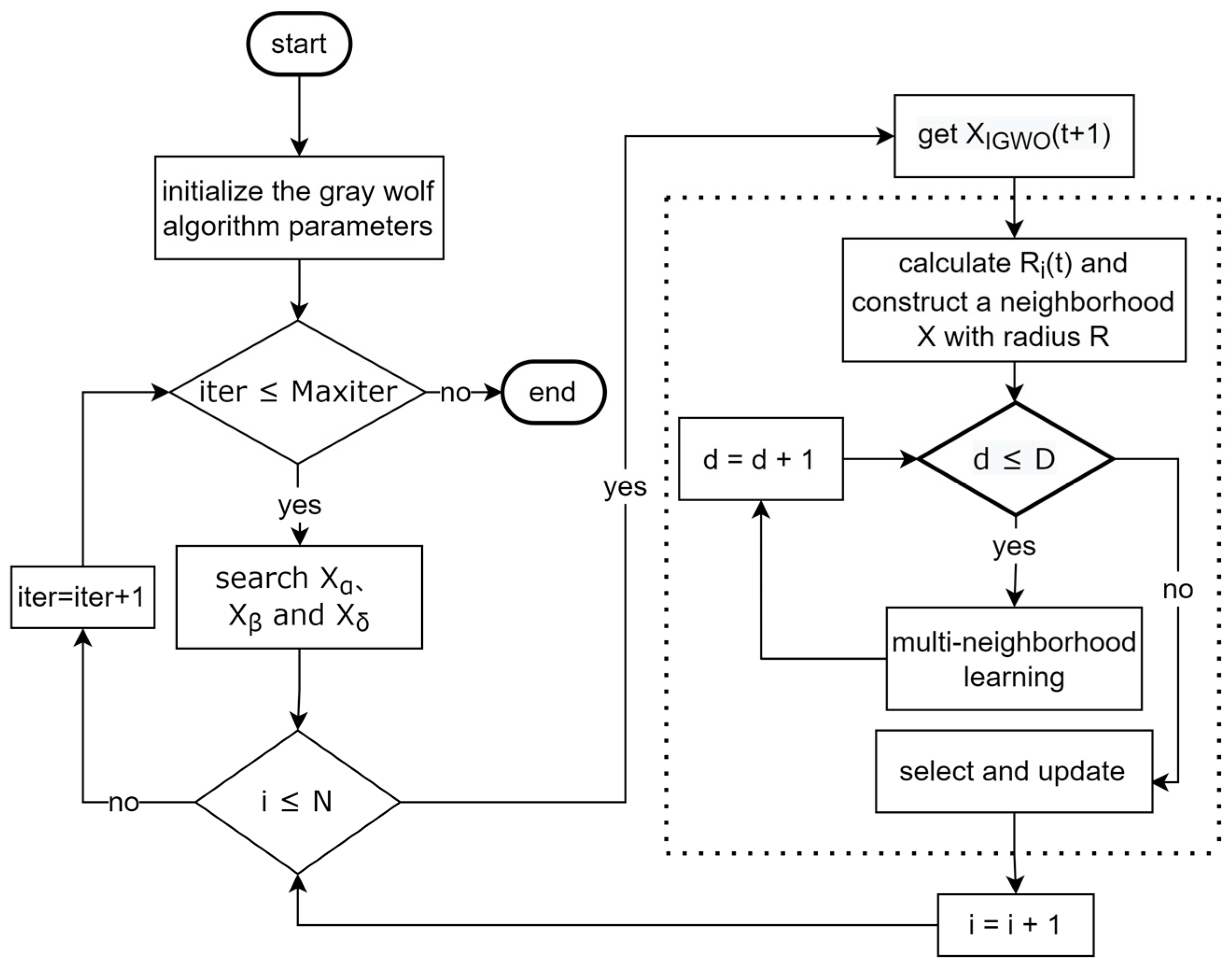
2.1. Improved Gray Wolf Optimization Algorithm

Gray wolf optimizer (GWO) simulates the predation behavior of gray wolf groups. Gray wolf groups have a strict hierarchy and a small number of gray wolves with the absolute right to speak lead a group of gray wolves toward their prey. GWO divides wolves into four levels based on fitness: α ,   β ,   δ and ω . α is the optimal solution, β is the suboptimal solution, δ is the best solution and ω is the candidate solution. The hunting process is guided by α ,   β ,   δ and ω follows α ,   β ,   δ to the prey. The position of the prey corresponds to the solution of the problem. GWO is superior to intelligent optimization algorithms such as particle swarm optimization algorithms and genetic algorithms in finding the global optimal solution. However, it is easy to fall into the local optimal solution, resulting in low convergence accuracy. To overcome these problems, this paper adopts the IGWO [18]. IGWO proposed a DLH to modify the search strategy associated with the selection and update steps. DLH constructs a neighborhood for each wolf, and wolves can share neighboring information with each other. IGWO can alleviate the lack of population diversity, the imbalance between development and exploration and the premature convergence of GWO algorithms. The IGWO algorithm process is shown in Figure 1. Inside the dotted box are improvements.
First, the parameters are initialized. N wolves are randomly distributed in the search space. The entire population of wolves is stored in a matrix P o p that has N rows and D columns, where D is the dimension of the problem. The position of the i -th wolf in the t -th iteration is expressed as:
X i ( t ) = x i 1 , x i 2 , , x i D , 0 i N .
Then, in the GWO search strategy, the top three wolves of P o p are considered to be α , β and δ . When 0 i N , not all wolves in the wolf pack have been searched, the GWO search is still carried out; when i > N , complete the GWO search to obtain the positions X α , X β and X δ of α ,   β and δ wolves. The first candidate X I G W O ( t + 1 ) for the new position of wolf obtained by determining the prey encircle with X α , X β and X δ . The DLH search strategy generates another candidate X I D L H ( t + 1 ) for the new position of the wolf X i ( t ) is calculated by Equation (2).
X I D L H , d ( t + 1 ) = X i , d ( t ) + r a n d × ( X n , d ( t ) X r , d ( t ) ) .
Among them, X n , d ( t ) is a random neighbor selected from the neighborhood N i ( t ) constructed by Equation (3), and X r , d ( t ) is a random wolf selected from P o p .
N i ( t ) = X i , d ( t ) | D i ( X i ( t ) , X j ( t ) ) R i ( t ) , X j ( t ) P o p ,
R i ( t ) = | | X i ( t ) X I G W O ( t + 1 ) | | ,  
where D i is the Euclidean distance between X i ( t ) and X j ( t ) , and R i ( t ) is the radius of the neighborhood. DLH uses the Euclidean distance between the current position of X i ( t ) and the candidate position X I G W O ( t + 1 ) to calculate the radius of the neighborhood by Equation (4).
X i ( t + 1 ) = X I G W O ( t + 1 ) , i f   f ( X I G W O ) < f ( X I D L H ) X I D L H ( t + 1 ) , i f   f ( X I G W O )   f ( X I D L H ) .
Finally, compare the fitness of X I G W O ( t + 1 ) and X I D L H ( t + 1 ) through Equation (5) and select a better candidate. If the fitness of the selected candidate is less than X i ( t ) , then update X i ( t ) with the selected candidate, otherwise X i ( t ) remains unchanged in P o p . After performing this process for all wolves, the iteration counter ( i t e r ) adds 1, and the search can be iterated until a predefined number of iterations ( M a x i t e r ) is reached.

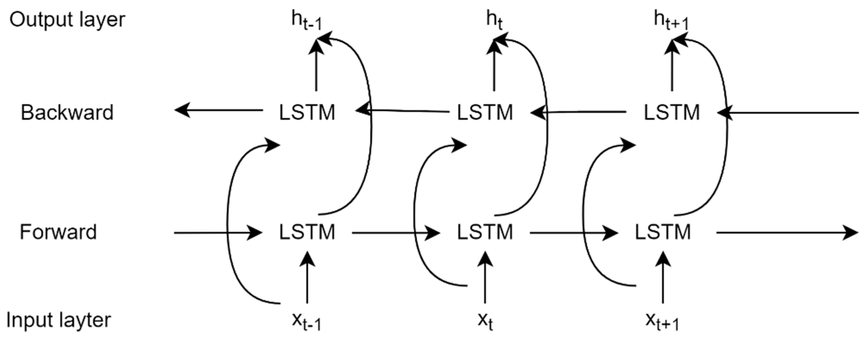
2.2. Bidirectional Long Short-Term Memory Network

BiLSTM considers both past and future characteristics of network traffic [19]. The hidden layer of BiLSTM consists of two parts: forward LSTM cell state and backward LSTM cell state. First, the network traffic data enters the hidden layer through the input layer to participate in the forward calculation and reverse calculation, respectively; Then, the data calculated by the hidden layer is passed to the output layer; Finally, the output layer fuses the forward LSTM output and the reverse LSTM output according to a certain weight to get the output result. The BiLSTM network structure is shown in Figure 2, where x t represents the input and h t represents the output of the network.

3. BiLSTM Attack Prediction Model Based on Improved Gray Wolf Algorithm

3.1. Model

Due to the good performance of deep learning in all aspects, literature [20,21,22] proposes a network attack prediction method based on deep learning. Literature [20] uses GRU to learn the data of past network attacks to predict future networks to achieve the purpose of network attack prediction. In this paper, the prediction model is named IGWO-BiLSTM, and the structure of the prediction model is shown in Figure 3. Each component is a refinement of the structure of the model. The input module processes the raw data; The data preprocessing module performs feature extraction and normalization; The IGWO-BiLSTM hidden layer consists of two layers of IGWO-BiLSTM and one Dropout layer, and the hidden layer trains network traffic data; Attack data training IGWO-BiLSTM to obtain an attack prediction model.
The IGWO-BiLSTM attack prediction model process is as follows:
  • The characteristics of normal network traffic have a certain regularity. When the change range of normal network traffic is abnormal, it can be judged that a network attack has occurred at this time. Literature [23] proposed the IPDCF, sampling the network at a time interval of Δ t = 1 min , using Equation (6) for data statistics, using Equation (7) for normalization and other data preprocessing operations:
    I P D C F i = T i < t < T i + 1 P t .
    Among them, I P D C F i is the i-th value in the time series and P is the data packet.
    x ^ = x x min x max x min .
    Among them, x ^ is the normalized value, x is the original value, x min is the minimum value and x max is the maximum value;
  • Sampling the data set at a time interval of Δ t = 1 min and calculating the IPDCF value of each sampling. After m times of sampling, time series T is obtained and Equation (8) is used for time series modeling:
    T = { I P D C F i , i = 1 , 2 , , M } ,
    Among them, M is the length of the data set, Δ t = 1 min ;
  • The raw data set is divided into a normal traffic data set and attack traffic data set. The normal traffic data set is used for prediction model training and prediction performance testing and the attack data set is used for attack experiments. Using sliding window technology, a window with a length of 60 and a width of 1 is selected, set the step size to 10 and perform sliding interception on the original network traffic data to obtain the network traffic training set and test set;
  • Initialize the parameters of the improved gray wolf algorithm. Randomly generate wolves, the total number N = 50 , the maximum number of iterations M a x i t e r = 10 , the dimension D of the problem is the number of BiLSTM optimization parameters D = 4 , the number of hidden layer units of BiLSTM ( n e u r o n s 1 , n e u r o n s 2 ) , the forgetting rate ( d r o p o u t ) and batch size ( b a t c h _ s i z e ) correspond to the parameter coordinates of the individual positions of wolves, set the upper and lower limits u b = [ 200 , 200 , 0.9 , 10 ] , l b = [ 32 , 32 , 0.1 , 1 ] ;
  • Initialize BiLSTM parameters and select a two-layer BiLSTM network. The number of hidden layer units ( n e u r o n s 1 , n e u r o n s 2 ) , dropout rate ( d r o p o u t ) and batch size ( b a t c h _ s i z e ) of BiLSTM are initialized to n e u r o n s 1 = 128 n e u r o n s 2 = 64 d r o p o u t = 0.4 b a t c h _ s i z e = 5 , the maximum number of iterations is 500 and the fitness function is the mean squared error ( M S E ) between the predicted value and the real value. Equation (9) was used to calculate the individual fitness of wolves and the fitness was returned to IGWO,
    M S E = 1 n i = 1 n ( Y i Y ^ i ) 2 .
    Among them, Y i is the real value and Y ^ i is the predicted value;
  • Normal network traffic time series input the model according to the window set in step (3) and train the model;
  • Use Equation (9) to calculate the fitness of each gray wolf. M S E is the expected value of the square of the difference between the real value and the predicted value. The greater the error, the greater the value. Select the three wolves with the smallest fitness, α ,   β ,   δ to search for GWO, update the position of other gray wolves ω to get the first candidate X I G W O ( t + 1 ) ;
  • Use Equation (2) to search for DLH and generate another candidate X I D L H ( t + 1 ) for the new position of wolf X i ( t ) . Equation (5) was used to compare the fitness of X I G W O ( t + 1 ) and X I D L H ( t + 1 ) and better candidates were selected. If the fitness of the selected candidate is less than X i ( t ) , update X i ( t ) with the selected candidate, otherwise X i ( t ) remains unchanged in P o p ;
  • Determine whether to iterate to the maximum number of iterations. If i t e r > M a x i t e r , execute (10), otherwise i t e r = i t e r + 1 , execute (6);
  • Output the position coordinates of α , that is, the optimal parameter combination of BiLSTM. α ( n e u r o n s 1 ,   n e u r o n s 2 ,   d r o p o u t ,   b a t c h _ s i z e ) input IGWO-BiLSTM training, obtain the optimized converged IGWO-BiLSTM network prediction model;
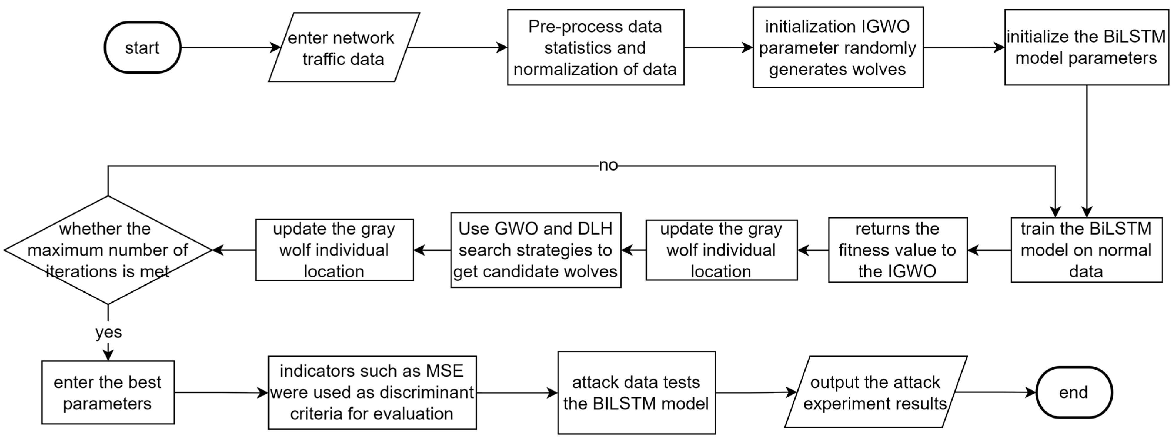
  • By inputting the network attack data into the prediction model and comparing the normal network traffic with the attack network traffic, the attack can be predicted in a timely and accurate manner. The flow chart of IGWO-BiLSTM is shown in Figure 4, each component represents a specific practice in the forecasting process and together constitutes the forecasting operation process.

3.2. Threshold Selection

In real life, people use the Internet in roughly the same way, so there will be a large number of users online at the same time. In this case, network congestion occurs, but the network congestion is different from that caused by DoS and DDoS. Because the fluctuating network traffic features extracted by IPDCF may be mistaken by the model as attack traffic, it is particularly critical to select an appropriate threshold for a given data set. If the threshold is too large, the DoS and DDoS alarm may be delayed or missed. If the threshold is too small, false positives may occur.
The IPDCFs of normal and predicted values were statistically analyzed to obtain their intervals [ a , b ] and [ c , d ] . Z is the maximum value of the IPDCF predicted value interval [ c , d ] , A is the average error between the predicted value and normal value, and the threshold is U = Z + A . According to Equation (10), when the predicted value X exceeds the preset threshold value U , it is considered abnormal traffic, and the existence of network attack behavior can be determined. When the deviation of the predicted value is large but does not exceed the preset threshold value U , normal network congestion except abnormal is considered to have occurred.
f X U , D O S   a t t a c k s   o r   D D O S   a t t a c k s o t h e r w i s e , n o r m a l   c o n g e s t i o n .

4. Experimental Simulation and Analysis

4.1. Data Set Selection

The simulation experiment selects three representative network traffic data sets: dedicated Internet service provider Internet traffic (ec_data); there are weeks of network traffic collected by the MIT Lincoln Laboratory, 1999 (DARPA99), of which the first week and the third week as training sample data and the second weeks as test sample data; DOS and DDOS data set collected by the MIT Lincoln Laboratory, 2000 (DARPA00). Among them, the ec_data and the DARPA99 are used for training and performance comparison of the prediction model to prove the universality of the prediction model, and the DARPA00 dataset is used for attack experiments. A detailed description of the above datasets is shown in Table 1.
As shown in Table 2, the ec_data has two columns. The first column is the number of the network traffic data, and the second column is the size of the network traffic in Mb.
As shown in Table 3, the DARPA99 collects TCPDUMP network connection data. The first column is the number of the network connection, the second column is the time when the connection occurred, the third and fourth columns are the source and destination address of the connection, the fifth column is the network protocol used by the connection and the sixth column is the length of the connection. The DARPA00 data set and the DARPA99 data set have the same structure and will not be repeated here.

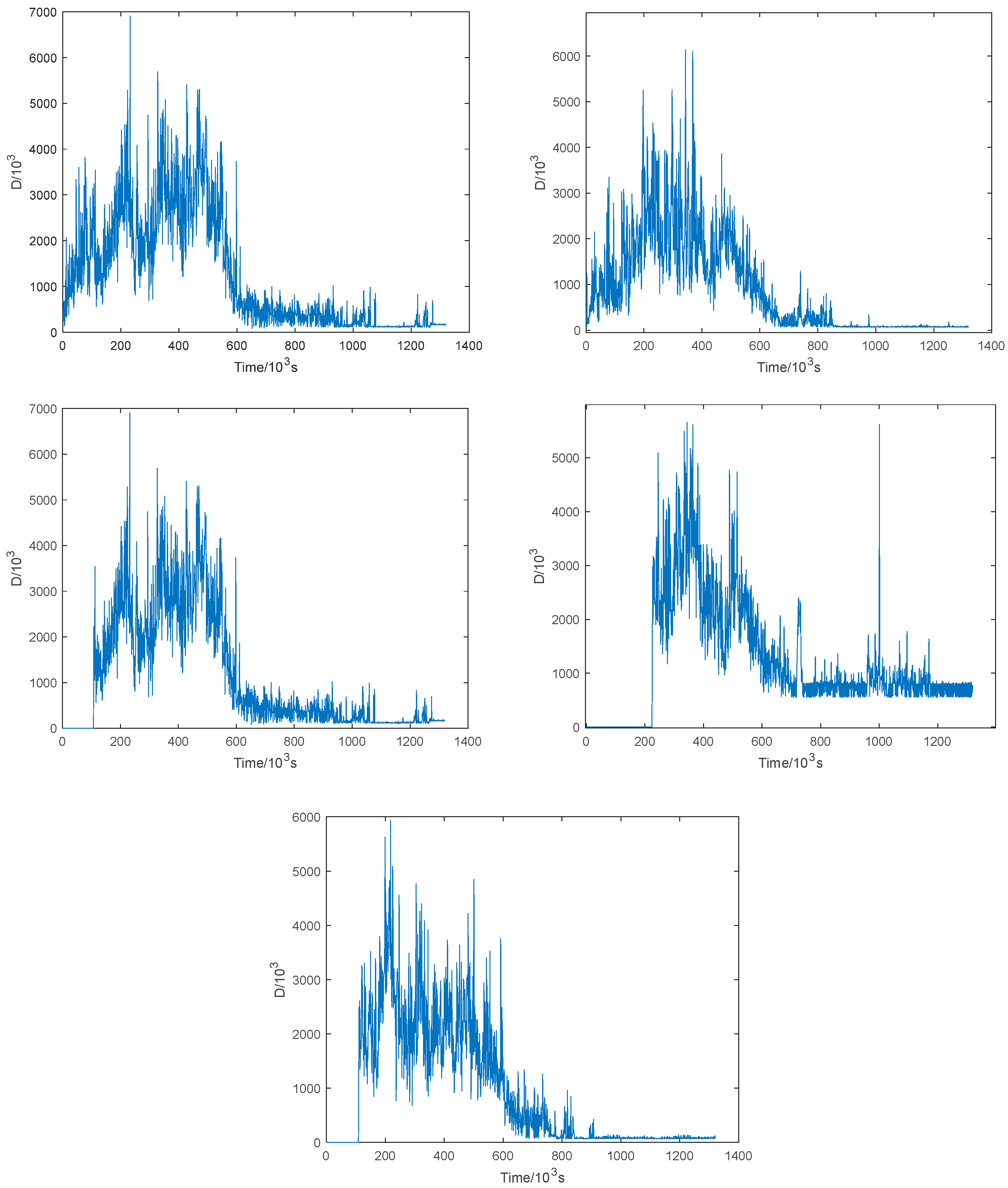
4.2. Feature Extraction and Analysis

ec_data compiled 14,772 sets of network traffic data from 6 July 2005 to 28 July 2005. Figure 5 shows the data obtained from the ec_data sampling at 5 minutes intervals. Network traffic in the ordinate is normalized. As can be seen from the figure, since people’s living habits are roughly the same, network traffic data is periodic on the macro level and it is found that network traffic data has the characteristics of frequent outbreaks on the micro level. Therefore, it is required that the prediction model can predict the sudden outbreak of network traffic.
The DARPA99 is the three-week training data provided by DARPA intrusion detection in 1999. The first and third weeks do not contain any attacks as training data and the second week contains a subset of 1998 attacks, as well as several new attacks as test data. DARPA99 was sampled at 1 min intervals, and the number of data packets per minute was obtained as data characteristics. Data characteristics of 5d in the first week were shown in Figure 6. D in the figure is the number of IP packets. It can be seen from the figure that the data at a fixed time every day in the first week presents a relatively fixed trend, which further proves the feasibility of prediction.

4.3. Predictive Model Performance Comparison

Different data sets used in the same prediction model can prove the universality of the model. In this experiment, two data sets, ec_data and DARPA99, were used to evaluate the performance of the prediction model, which proves that the proposed model can be extended to different scenarios. In this paper, M S E , root mean square error ( R M S E ), mean absolute error ( M A E ) and coefficient of determination ( R 2 ) are selected as evaluation indexes. It is used to compare the prediction performance of the improved grey wolf optimization RNN (IGWO-RNN), the improved grey wolf optimization LSTM (IGWO-LSTM), the improved grey wolf optimization GRU (IGWO-GRU) and the improved grey wolf optimization BiLSTM (IGWO-BiLSTM) proposed in this paper. Among them, M S E ,   R M S E and M A E are as small as possible, and larger R 2 indicates that the model fitting effect is better. R 2 is used to indicate the degree of correlation between the real value and the predicted value, and the value range is 0 ~ 1 . If R 2 = 1 , the model fitting effect is poor; if R 2 = 0 , the model is perfect.

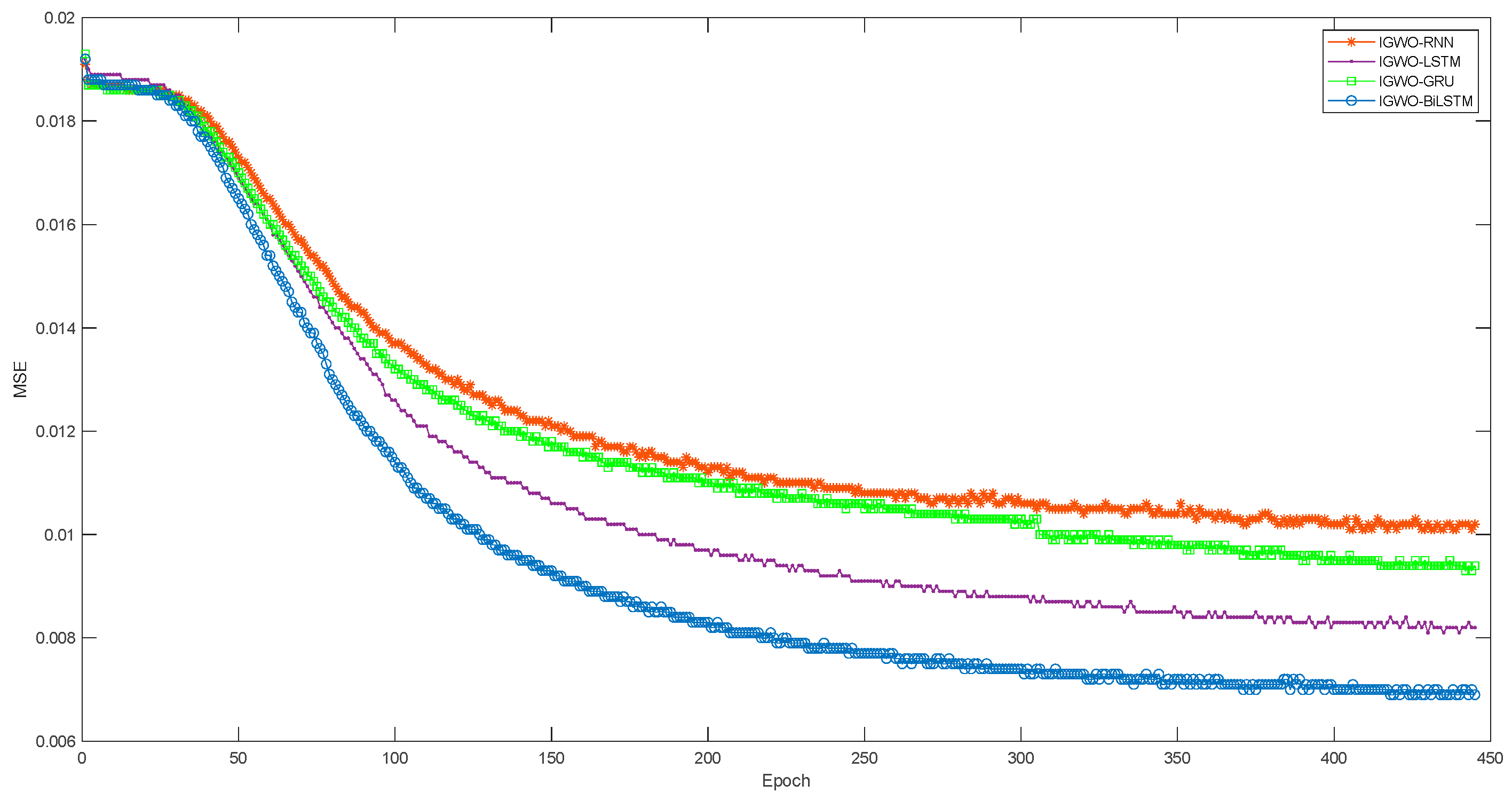
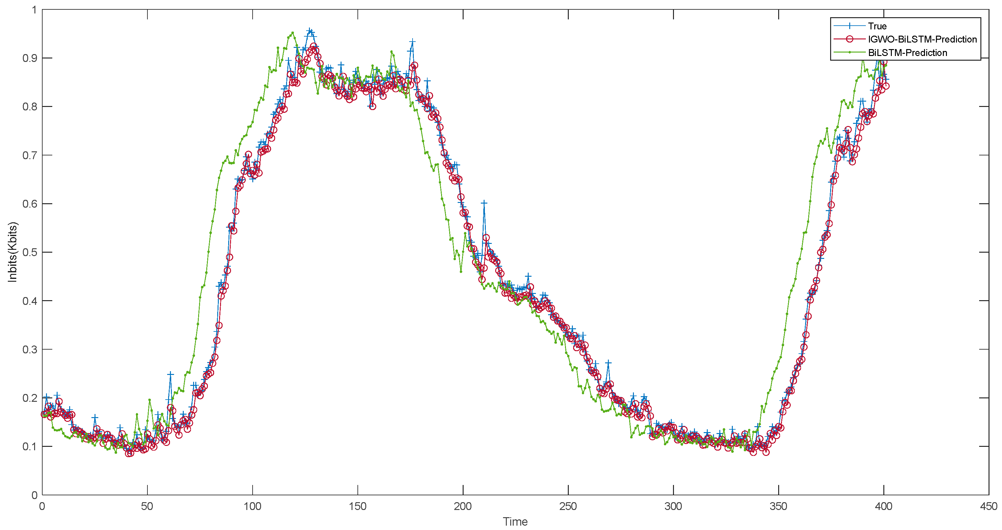
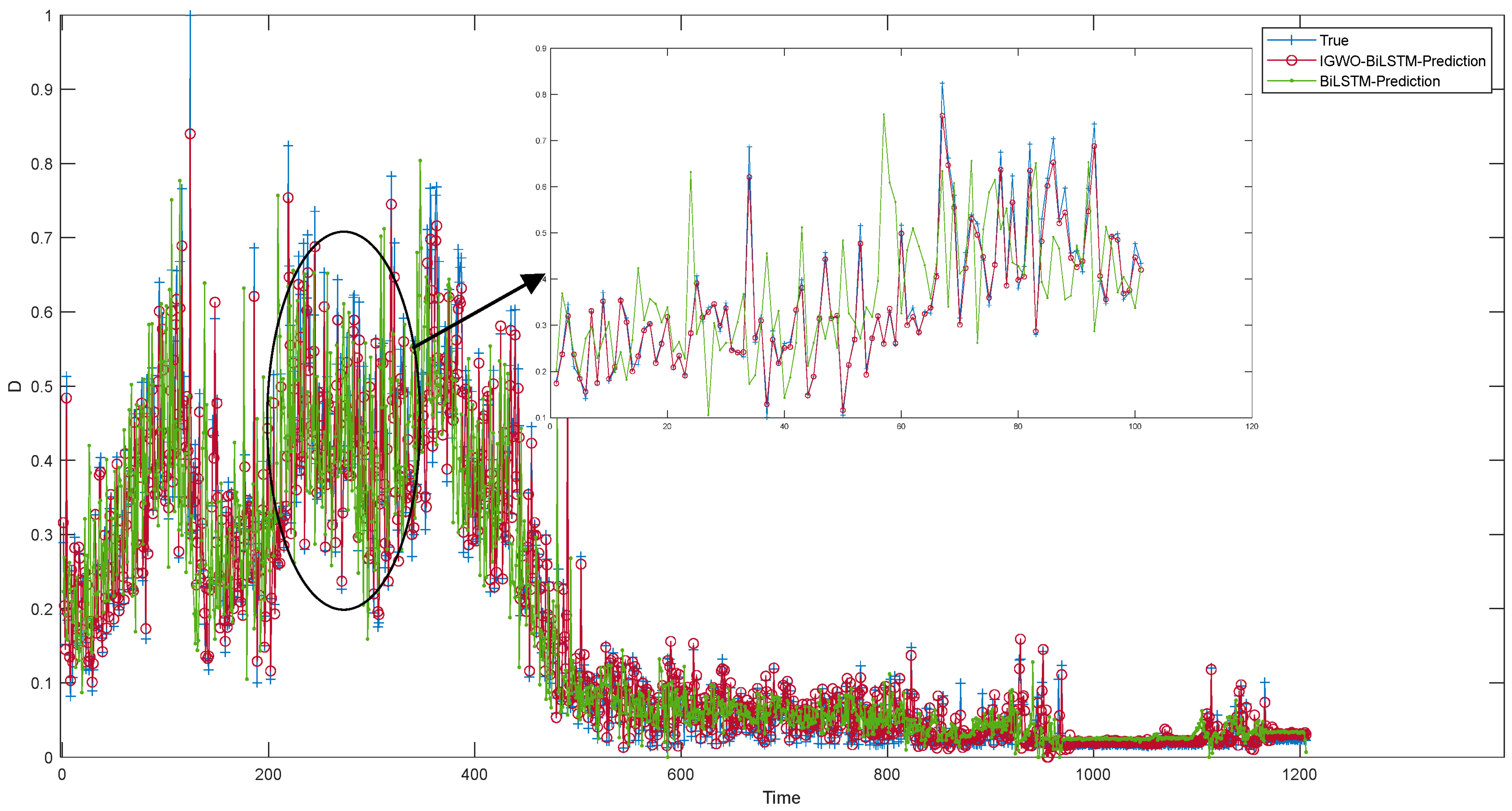
4.3.1. ec_data Data Set Prediction Model Performance Display

This section introduces the model’s performance on ec_data from three aspects. Firstly, the comparison of the time consumption between the original BiLSTM and IGWO-BiLSTM. It is found that the prediction efficiency of IGWO-BiLSTM is higher. Then, IGWO was applied to the RNN, LSTM, GRU and BiLSTM models. The decrease trend M S E was compared for 450 iterations, and it was found that the proposed model had the smallest M S E . Finally, the comparison graph between the predicted value and the real value of the IGWO-BiLSTM model is shown. Through observation, it is found that the prediction model can capture the change rule of the real value and make an accurate prediction.
As shown in Figure 7, the time-consuming ec_data data set runs 10 times on IGWO-LSTM and BiLSTM models. Compared with the LSTM model, IGWO-BiLSTM reduces the total time of 10 iterations by 186s, and the average time of each iteration is reduced by 18.6s. The reduced time can be used to predict network trends in advance, to respond to network attacks promptly, which is of great significance in practical applications.
As shown in Figure 8, the M S E change trend of IGWO in the iteration of RNN, LSTM, GRU and BiLSTM models during the training process ec_data the training process. Through comparison, IGWO-BiLSTM was found to have the lowest M S E . The MSE eventually stabilized, and IGWO-BiLSTM, IGWO-RNN, IGWO-LSTM and IGWO-GRU reached 0.0069, 0.0102, 0.0082 and 0.0094, respectively, and IGWO-BiLSTM decreased by 0.0033, 0.0013 and 0.0025 compared with IGWO-RNN, IGWO-LSTM and IGWO-GRU, respectively.
Figure 9 shows the local comparison between the predicted values and the real values of ec_data on IGWO-BiLSTM. The horizontal axis is sampling time, and the vertical axis is the network traffic data unit. It can be found that the IGWO-BiLSTM model can better capture the changing trend of the real network flow than the BiLSTM model, and the predicted value obtained is closer to the real value and the prediction accuracy is improved to 98.71%.

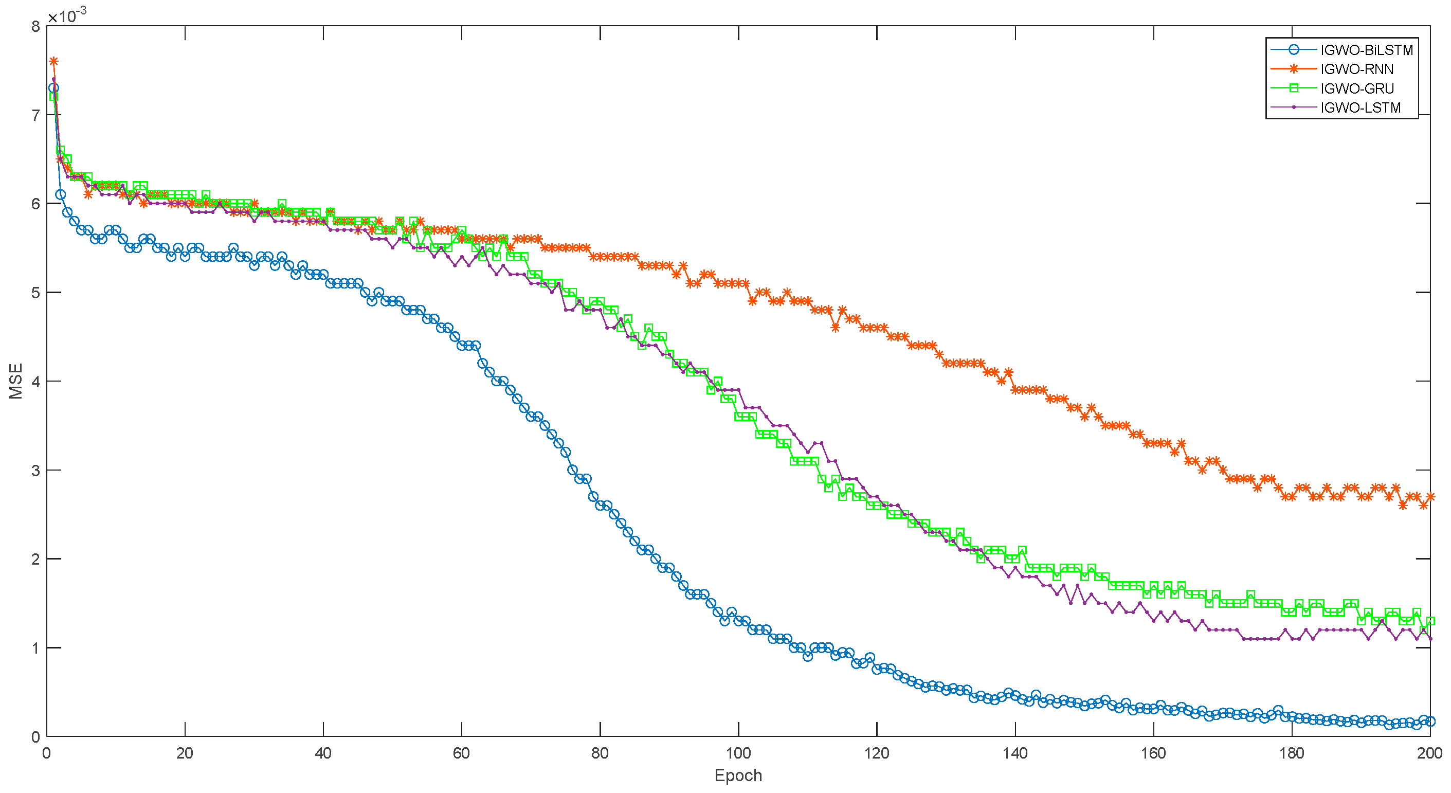
4.3.2. DARPA99 Data Set Prediction Model Performance Display

This section describes how the model performs on DARPA99 in three ways. First, IGWO is applied to M S E comparison between other neural network models and BiLSTM models. Then, the comparison of the predicted value of DARPA99 with the real value on the IGWO-BiLSTM model is displayed. Finally, R M S E , R 2 and M A E of IGWO-BiLSTM and other models are compared.
As shown in Figure 10, the trend of M S E change of IGWO during RNN, LSTM, GRU and BiLSTM iterations during DARPA99 training. Through comparison, it was found that IGWO-BiLSM had the smallest M S E . The M S E eventually plateaued, with IGWO-BiLSTM, IGWO-RNN, IGWO-LSTM and IGWO-GRU reaching 0.000169, 0.0027, 0.0011 and 0.0013, respectively.
As shown in Figure 11, the real value of DARPA99 is compared with the predicted value on IGWO-BiLSTM. When real network traffic suddenly breaks out, IGWO-BiLSTM can catch the change in time and accurately output the predicted value in time. Through experiments, it is found that the predicted value obtained by the IGWO-BiLSTM model is closer to the real value than the predicted value obtained by the BiLSTM model, which confirms that the IGWO-BiLSTM model has better predictive performance, so the subsequent attack experiment can be carried out.
It can be seen from Table 4 that R M S E , R 2 and M A E values of IGWO-BiLSTM are optimal. Compared with IGWO-RNN, IGWO-LSTM and IGWO-GRU, R 2 increased by 0.33, 0.57 and 0.06, respectively.

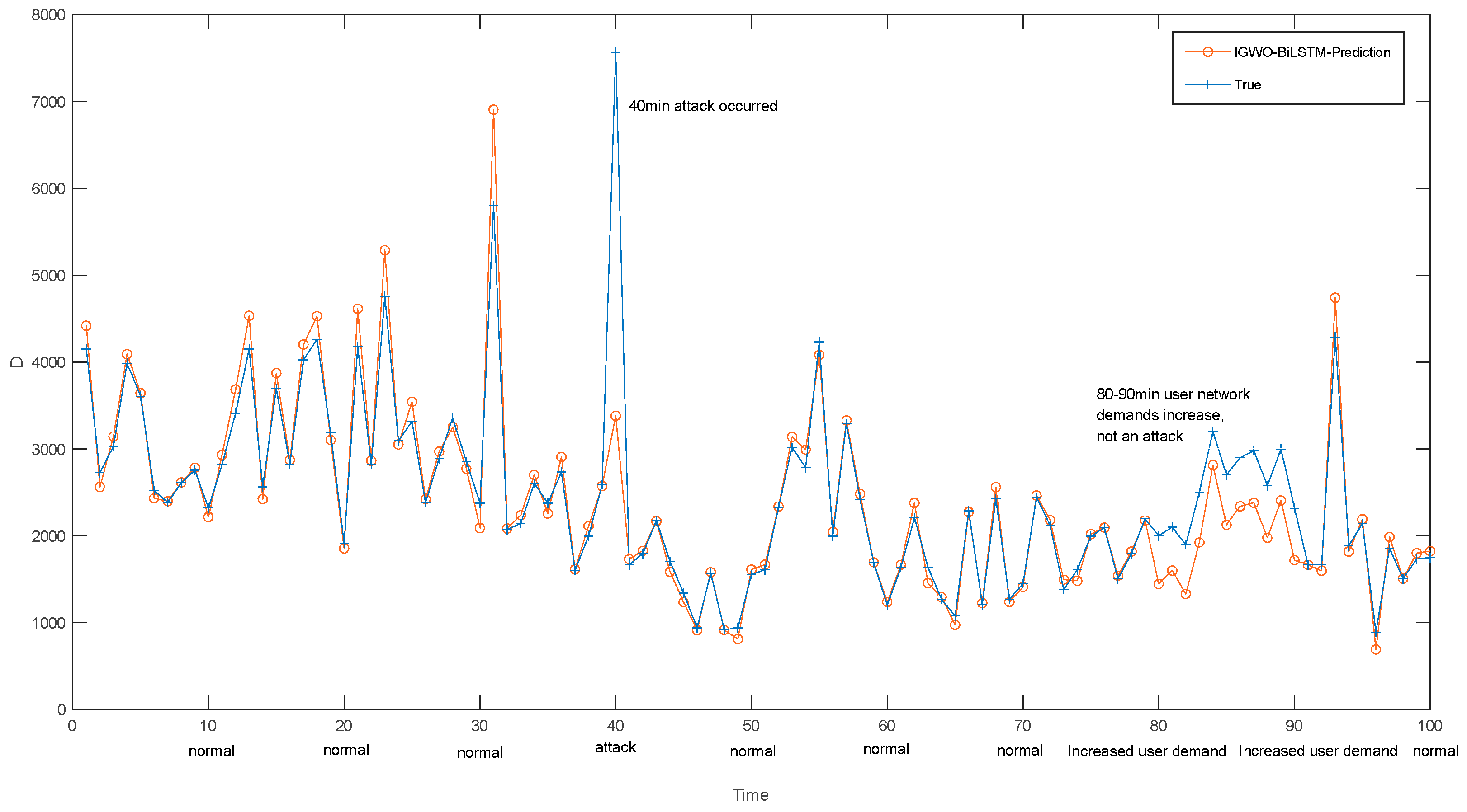
4.4. Network Attack Detection and Analysis

Network attack prediction is realized by combining network traffic prediction with threshold setting. The current network traffic is input into IGWO-BiLSTM to get the future network traffic and the predicted value is compared with the threshold value to judge whether the network attack occurs. In normal cases, the IPDCF value of network traffic is small, but in attack time, the IPDCF value of network traffic is large. By counting the interval between normal flow and predicted characteristic values, the threshold U is calculated to be 7184. When the predicted value exceeds 7184, a network attack can be identified. Due to the large types of attacks and inconsistent attack judgment methods, this paper can predict and identify the network traffic under attack by setting thresholds. Specific categories of attacks will be realized in the next experiment.
As can be seen from Figure 12, in the 40 min, the predicted value exceeds the threshold, which determines that a network attack occurs at this time. In the 80th to 90th minute, although the deviation between the real value and the predicted value is large, it does not exceed the threshold. Therefore, it is judged not as a network attack, but as the actual network demand of users increases at this time to avoid false positives.

4.5. Discussion

The rapid development of networks leads to higher requirements for network security. The current academic research on network attack focuses on the analysis of network security event logs detected by network security facilities. In addition, the network attack prediction technology is the most important. Therefore, this paper proposes IGWO-BiLSTM for network attack prediction. As an intelligent optimization algorithm, IGWO can solve engineering problems, optimization problems and applications in neural networks. Meanwhile, compared with GWO and particle swarm optimization algorithms, IGWO has the advantages of global search and has corresponding research value.
IGWO-BiLSTM used ec_data and DARPA99 to verify the prediction effect. Firstly, compared with BiLSTM, IGWO-BiLSTM greatly shortens the time of network traffic prediction. In practical application, it can provide faster response decisions and effectively reduce the damage to network equipment. Secondly, this model can converge earlier to lower Loss than other models. Loss is defined by MAE, which represents the difference between the predicted value and the true value. Compared with IGWO-RNN, IGWO-LSTM and IGWO-GRU, IGWO-BiLSTM decreased by 0.0033, 0.0013 and 0.00255, respectively. Finally, compared with IGWO-RNN, IGWO-LSTM and IGWO-GRU, the accuracy of IGWO-BiLSTM is improved by 0.33, 0.57 and 0.06, respectively.

5. Conclusions

In our daily life, cyber-attacks can happen at any time and bring about serious consequences. Therefore, the IGWO-BiLSTM network attack prediction model is proposed to study the potential attack behavior in the network. Specifically, the IGWO method is used in this paper to solve the problems of slow convergence of the original GWO, premature loss of diversity of the population and easily falling into the local optimum. IGWO-BiLSTM is used to predict normal network traffic and set a reasonable threshold to identify the anomalies caused by network attacks. The experimental results show that the reconstruction error between the predicted value and the real value is minimal, and the prediction performance of the proposed method is better than that of RNN, LSTM, GRU, etc.
IGWO has solved the problem of slow convergence and poor prediction accuracy of BiLSTM from the parameter. However, the prediction effect of BiLSTM still has a large room for improvement. In addition, this paper only discusses IGWO-BiLSTM’s predictive performance on ec_data and DARPA99 and does not apply it to physical layer devices. Subsequent research should try to use different network models to predict network traffic and apply them to physical layer attacks such as signal interference or resource hiding.

Author Contributions

Conceptualization, S.Q. and Y.W.; methodology, S.Q.; software, Y.W.; validation, Y.L., Y.W. and F.C.; formal analysis, J.Z.; investigation, F.C.; resources, S.Q.; data curation, Y.L.; writing—original draft preparation, Y.W.; writing—review and editing, S.Q., Y.W. and Y.L.; visualization, Y.W.; supervision, Y.L.; project administration, Y.L.; funding acquisition, S.Q. and Y.L. All authors have read and agreed to the published version of the manuscript.

Funding

This research was funded by the fund project of the Equipment Development Department of the Central Military Commission grant number [No.6140002010101, No.6140001030111], and the APC was funded by Dalian University.

Institutional Review Board Statement

Not applicable.

Informed Consent Statement

Not applicable.

Data Availability Statement

The processed data required to reproduce these findings cannot be shared as the data also forms part of an ongoing study.

Conflicts of Interest

The authors declare no conflict of interest.

References

  1. Roshan, K.; Zafar, A. Deep learning approaches for anomaly and intrusion detection in computer network: A review. In Cyber Security and Digital Forensics: Proceedings of ICCSDF; Springer: Singapore, 2021; Volume 73, pp. 551–563. [Google Scholar]
  2. Jian, S.J.; Lu, Z.G.; Du, D. Overview of network intrusion detection technology. J. Cyber Secur. 2020, 5, 96–122. [Google Scholar]
  3. Cheema, A.; Tariq, M.; Hafiz, A. Prevention Techniques against Distributed Denial of Service Attacks in Heterogeneous Networks: A Systematic Review. Secur. Commun. Netw. 2022, 2022, 8379532. [Google Scholar] [CrossRef]
  4. Black, S.; Kim, Y. An Overview on Detection and Prevention of Application Layer DDoS Attacks. In Proceedings of the IEEE 12th Annual Computing and Communication Workshop and Conference (CCWC), Las Vegas, NV, USA, 26–29 January 2022; pp. 791–800. [Google Scholar]
  5. Zheng, Y.; Li, Z.; Xu, X. Dynamic defenses in cyber security: Techniques, methods and challenges. Digit. Commun. Netw. 2022, 8, 422–435. [Google Scholar] [CrossRef]
  6. Lohrasbinasab, I.; Shahraki, A.; Taherkordi, A. From statistical-to machine learning-based network traffic prediction. Trans. Emerg. Telecommun. Technol. 2022, 33, e4394. [Google Scholar] [CrossRef]
  7. Fan, J.; Mu, D.; Liu, Y. Research on network traffic prediction model based on neural network. In Proceedings of the 2nd International Conference on Information Systems and Computer Aided Education (ICISCAE), Dalian, China, 28–30 September 2019; pp. 554–557. [Google Scholar]
  8. Laurenti, L.; Tinti, E.; Galasso, F. Deep learning for laboratory earthquake prediction and autoregressive forecasting of fault zone stress. Earth Planet. Sci. Lett. 2022, 598, 117825. [Google Scholar] [CrossRef]
  9. Siqueira, H.; Belotti, J.T.; Boccato, L. Recursive linear models optimized by bioinspired metaheuristics to streamflow time series prediction. Int. Trans. Oper. Res. 2023, 30, 742–773. [Google Scholar] [CrossRef]
  10. Alzahrani, S.I.; Aljamaan, I.A.; AI-Fakin, E.A. Forecasting the spread of the COVID-19 pandemic in Saudi Arabia using ARIMA prediction model under current public health interventions. J. Infect. Public Health 2020, 13, 919. [Google Scholar] [CrossRef] [PubMed]
  11. Huang, C.W.; Chiang, C.T.; Li, Q. A study of deep learning networks on mobile traffic forecasting. In Proceedings of the 2017 IEEE 28th Annual International Symposium on Personal, Indoor, and Mobile Radio Communications (PIMRC), Montreal, QC, Canada, 8–13 October 2017; pp. 1–6. [Google Scholar]
  12. Sebastian, K.; Gao, H.; Xing, X. Utilizing an Ensemble STL Decomposition and GRU Model for Base Station Traffic Forecasting. In Proceedings of the 2020 59th Annual Conference of the Society of Instrument and Control Engineers of Japan (SICE), Chiang Mai, Thailand, 23–26 September 2020; IEEE: Piscataway, NJ, USA, 2020; pp. 314–319. [Google Scholar]
  13. Trinh, H.D.; Giupponi, L.; Dini, P. Mobile traffic prediction from raw data using LSTM networks. In Proceedings of the 2018 IEEE 29th Annual International Symposium on Personal, Indoor and Mobile Radio Communications (PIMRC), Bologna, Italy, 9–12 September 2018; Volume 25, pp. 1827–1832. [Google Scholar]
  14. Bi, J.; Zhang, X.; Yuan, H. A Hybrid Prediction Method for Realistic Network Traffic With Temporal Convolutional Network and LSTM. IEEE Trans. Autom. Sci. Eng. 2022, 19, 1869–1879. [Google Scholar] [CrossRef]
  15. Lu, S.; Zhang, Q.; Chen, G. A combined method for short-term traffic flow prediction based on recurrent neural network. Alex. Eng. J. 2021, 60, 87–94. [Google Scholar] [CrossRef]
  16. Ramakrishnan, N.; Soni, T. Network traffic prediction using recurrent neural networks. In Proceedings of the 17th IEEE International Conference on Machine Learning and Applications (ICMLA), Orlando, FL, USA, 17–20 December 2018; pp. 187–193. [Google Scholar]
  17. Siami-Namini, S.; Tavakoli, N.; Namin, A.S. The performance of LSTM and BiLSTM in forecasting time series. In Proceedings of the 2019 IEEE International Conference on Big Data (Big Data), Los Angeles, CA, USA, 9–12 December 2019; pp. 3285–3292. [Google Scholar]
  18. Nadimi-Shahraki, M.H.; Taghian, S.; Mirjalili, S. An improved grey wolf optimizer for solving engineering problems. Expert Syst. Appl. 2021, 166, 113917. [Google Scholar] [CrossRef]
  19. Lin, Z.; Sun, X.; Ji, Y. Landslide displacement prediction based on time series analysis and Double-BiLSTM Model. Int. J. Environ. Res. Public Health 2022, 19, 2077. [Google Scholar] [CrossRef] [PubMed]
  20. Ansari, M.S.; Bartos, V.; Lee, B. Shallow and Deep Learning Approaches for Network Intrusion Alert Prediction. Procedia Comput. 2020, 171, 644–653. [Google Scholar] [CrossRef]
  21. Ansari, M.S.; Bartoš, V.; Lee, B. GRU-based deep learning approach for network intrusion alert prediction. Future Gener. Comput. Syst. 2022, 128, 235–247. [Google Scholar] [CrossRef]
  22. Bartos, V.; Zadnik, M.; Habib, S.M.; Vasilomanolakis, E. Network entity characterization and attack prediction. Future Gener. Comput. Syst. 2019, 97, 674–686. [Google Scholar] [CrossRef] [Green Version]
  23. Cheng, J.; Luo, Y.; Tang, X.; Ou, M. DDoS attack detection method based on LSTM traffic prediction. J. Huazhong Univ. Sci. Technol. (Nat. Sci. Ed.) 2019, 47, 32–36. [Google Scholar]
Figure 1. IGWO flowchart.
Applsci 13 06871 g001
Figure 2. BiLSTM network structure.
Applsci 13 06871 g002
Figure 3. IGWO-BiLSTM model structure.
Applsci 13 06871 g003
Figure 4. IGWO-BiLSTM flow chart.
Applsci 13 06871 g004
Figure 5. Normalization of ec_data dataset.
Applsci 13 06871 g005
Figure 6. Schematic diagram of DARPA99 first week 5d data features.
Applsci 13 06871 g006
Figure 7. Time-consuming comparison of 10 iterations.
Applsci 13 06871 g007
Figure 8. MSE trend graph of ec_data dataset.
Applsci 13 06871 g008
Figure 9. Local comparison between the real value and predicted value of ec_data.
Applsci 13 06871 g009
Figure 10. DARPA99 dataset IGWO optimization network loss diagram.
Applsci 13 06871 g010
Figure 11. DARPA99 real value and predicted value comparison chart.
Applsci 13 06871 g011
Figure 12. Simulation attack experiment results.
Applsci 13 06871 g012
Table 1. Dataset description.
Dataset NameThe Amount of DataData UnitStatistical Interval
ec_data14,772Mb5 min
DARPA9919,800IPDCF1 min
DARPA0025IPDCF1 min
Table 2. ec_data dataset.
No.Network Traffic
13,562,279,127
23,710,215,571
33,877,469,703
43,876,354,871
54,582,542,581
65,016,336,869
Table 3. DARPA99 dataset.
No.TimeSourceDestinationProtocolLength
10.00000HewlettP_61:aa:c9HewlettP_61:aa:c9LLC54
20.346281192.168.1.30172.16.112.100SNMP146
30.347844172.16.112.100192.168.1.30SNMP159
41.499118HewlettP_61:aa:c9HewlettP_61:aa:c9LLC54
52.341313192.168.1.30172.16.112.100SNMP146
62.342837172.16.112.100192.168.1.30SNMP159
Table 4. Comparison of improved algorithms to optimize network performance.
MethodRMSER2MAE
IGWO-RNN0.04830.66880.0443
IGWO-LSTM0.05290.42630.0326
IGWO-GRU0.03520.93130.0259
IGWO-BiLSTM0.00940.99050.0200
Disclaimer/Publisher’s Note: The statements, opinions and data contained in all publications are solely those of the individual author(s) and contributor(s) and not of MDPI and/or the editor(s). MDPI and/or the editor(s) disclaim responsibility for any injury to people or property resulting from any ideas, methods, instructions or products referred to in the content.

