
FCP2Vec: Deep Learning-Based Approach to Software Change Prediction by Learning Co-Changing Patterns from Changelogs

Abstract
:1. Introduction
2. Materials and Methods
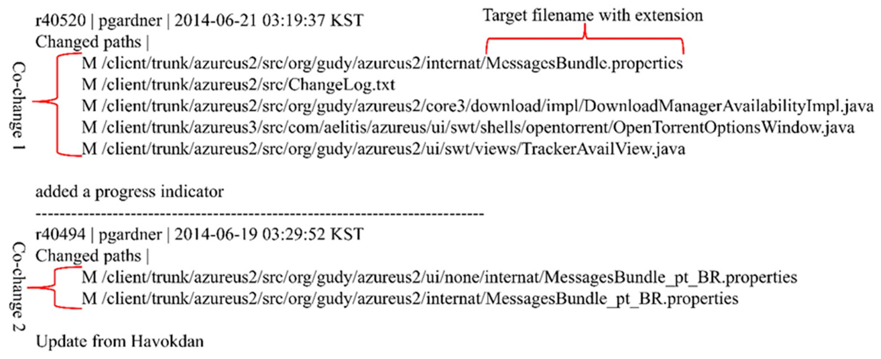
2.1. Leveraging Changelog Data in Change Propagation
2.2. Neural Language Model
3. Background
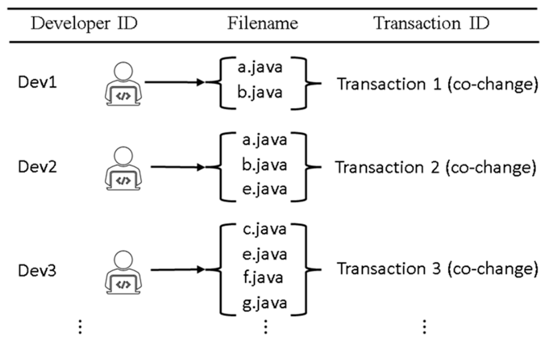
3.1. Problem Definition
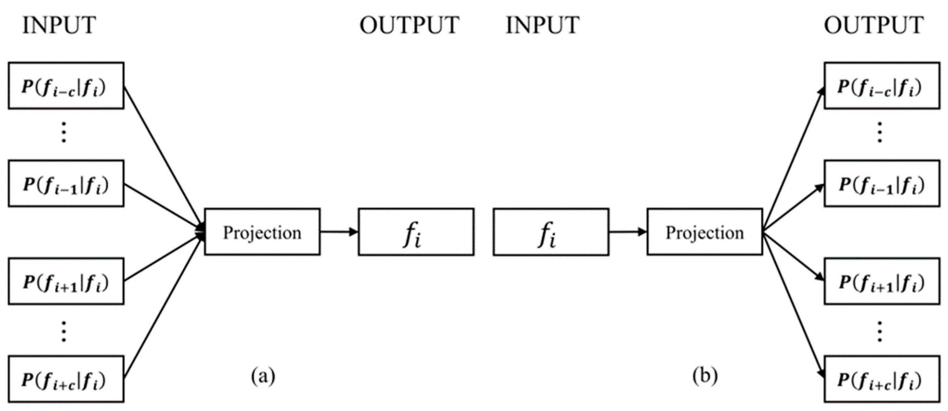
3.2. Word2vec
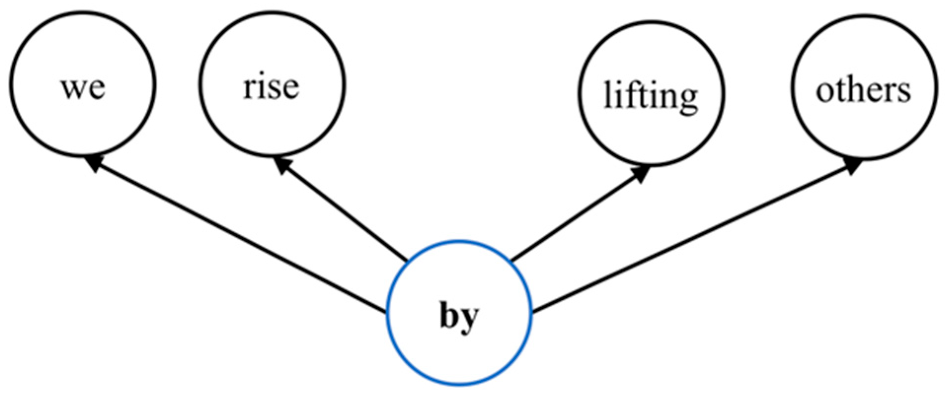
Skip-Gram
4. Proposed Approach
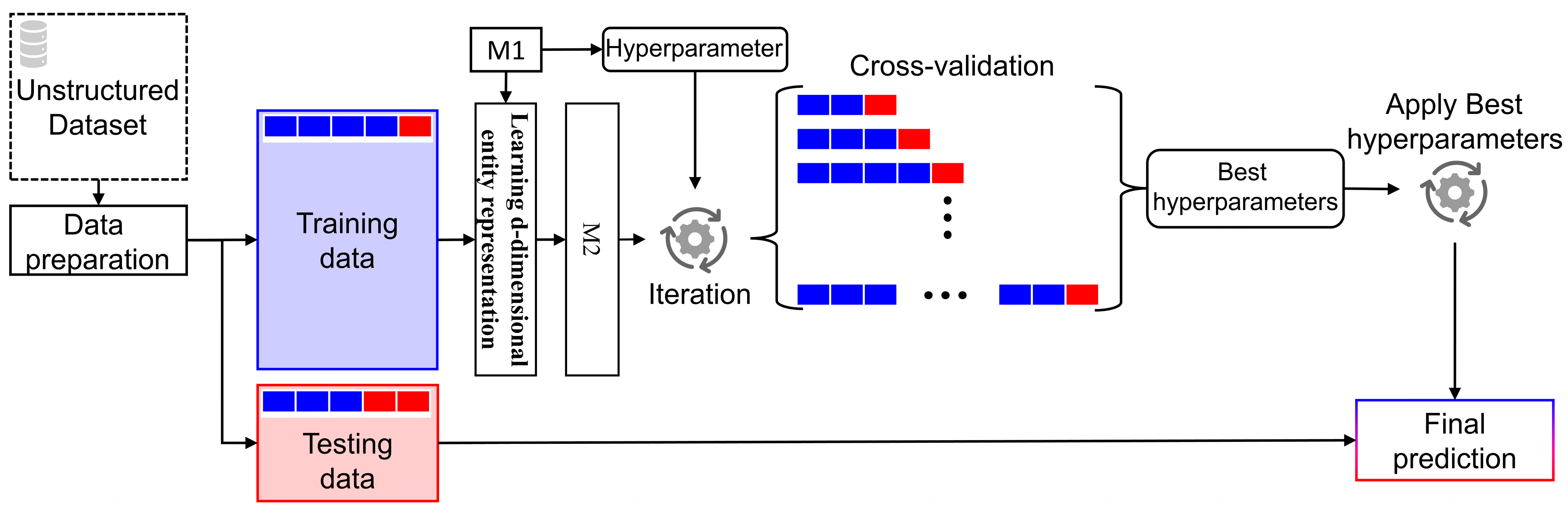
4.1. Data Preparation
4.2. Data Splitting
4.3. Learning D-Dimensional Element Representation
4.4. Evaluation Metrics
- Hit ratio at K (HR@K). It is equal to if the test element appears in the top list of predicted elements [70].
- Normalized discounted cumulative gain (NDCG@K). It considers both the order and relevance of the results. NDC@K favors higher ranks in the ordered list of predicted elements [71]. Since we consider that the ideal NDCG@K for a list retrieved from the UNN is 1, where is the position of the relevant element in the retrieved list. The higher the position in the retrieved list, the more favorable it is.
4.5. Hyperparameters
5. Empirical Studies
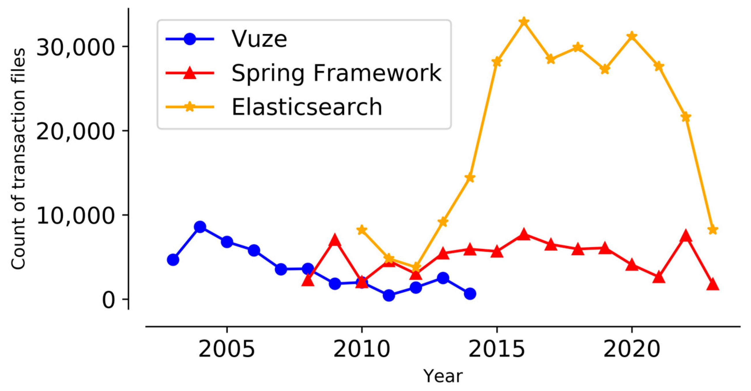
5.1. Transaction Data
5.2. System Environments
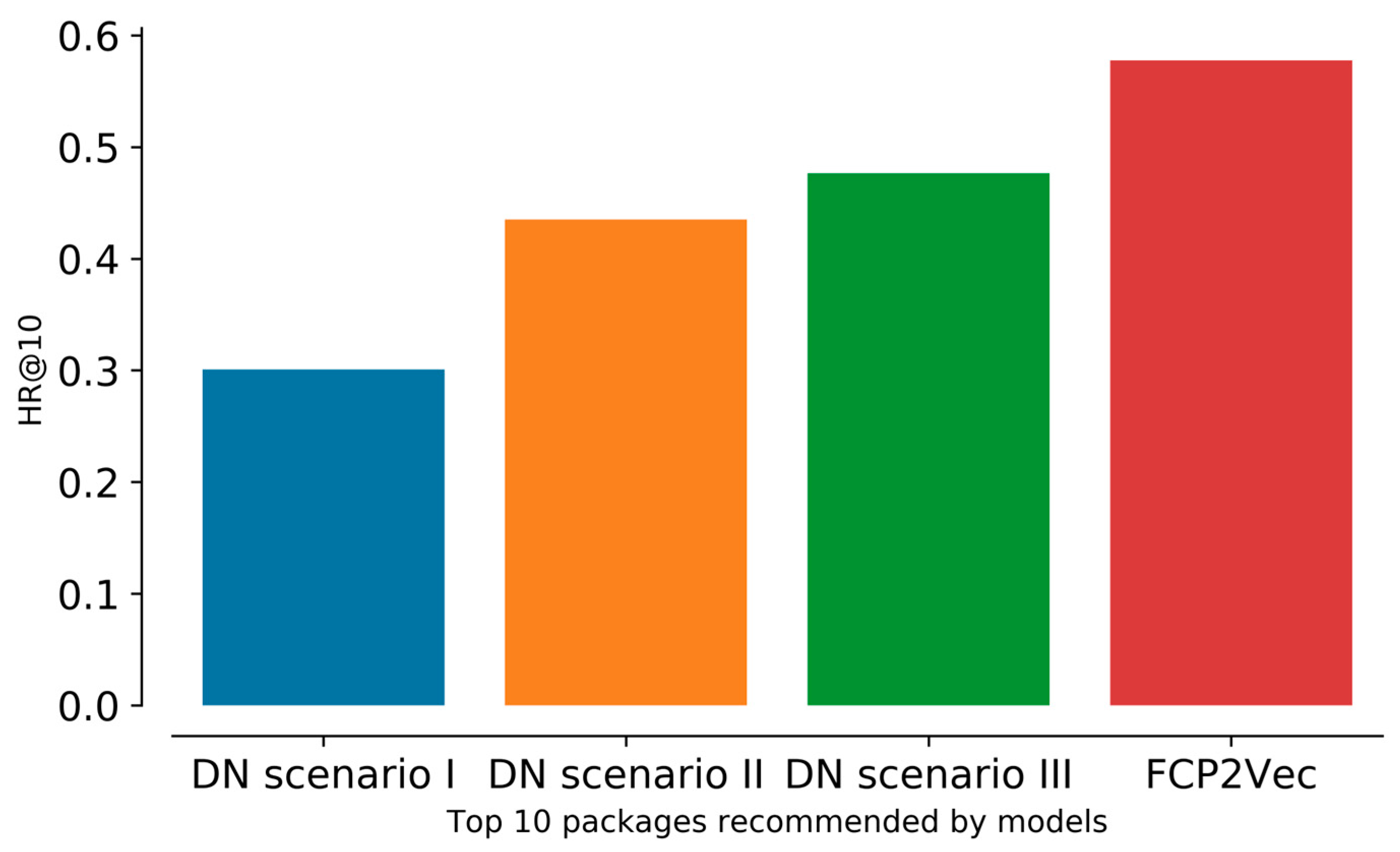
5.3. Results and Discussion
Comparison between FCP2Vec and DN
6. Conclusions
Author Contributions
Funding
Institutional Review Board Statement
Informed Consent Statement
Data Availability Statement
Conflicts of Interest
References
- Bennett, K.H.; Rajlich, V.T.; Wilde, N. Software Evolution and the Staged Model of the Software Lifecycle. In Advances in Computers; Elsevier: Amsterdam, The Netherlands, 2002; pp. 1–54. [Google Scholar]
- Yau, S.S.; Nicholl, R.A.; Tsai, J.J.-P.; Liu, S.-S. An Integrated Life-Cycle Model for Software Maintenance. IEEE Trans. Softw. Eng. 1988, 14, 1128–1144. [Google Scholar] [CrossRef]
- Rajlich, V. A model for change propagation based on graph rewriting. In Proceedings of the 1997 Proceedings International Conference on Software Maintenance, Bari, Italy, 1–3 October 1997. [Google Scholar]
- Yu, L.; Schach, S.R. Applying association mining to change propagation. Int. J. Softw. Eng. Knowl. Eng. 2008, 18, 1043–1061. [Google Scholar] [CrossRef]
- Pan, W.; Jiang, H.; Ming, H.; Chai, C.; Chen, B.; Li, H. Characterizing Software Stability via Change Propagation Simulation. Complexity 2019, 2019, 9414162. [Google Scholar] [CrossRef]
- Oliva, G.A.; Gerosa, M.A. Chapter 11—Change Coupling Between Software Artifacts: Learning from Past Changes. In The Art and Science of Analyzing Software Data; Morgan Kaufmann: Burlington, MA, USA, 2015; pp. 285–323. [Google Scholar]
- Ball, T.; Kim, J.H.; Porter, A.; Siy, H. If Your Version Control System Could Talk. In Proceedings of the ICSE Workshop Process Modelling and Empirical Studies of Software Engineering, Boston, MA, USA, 18 May 1997. [Google Scholar]
- Cataldo, M.; Herbsleb, J.D. Coordination breakdowns and their impact on development productivity and software failures. IEEE Trans. Softw. Eng. 2013, 39, 343–360. [Google Scholar] [CrossRef]
- Hassan, A.; Holt, R. Predicting Change Propagation in Software Systems. In Proceedings of the 20th IEEE International Conference on Software Maintenance, Chicago, IL, USA, 11–14 September 2004. [Google Scholar]
- Zimmermann, T.; Weißgerber, P.; Diehl, S.; Diehl, S. Mining version histories to guide software changes. IEEE Trans. Softw. Eng. 2005, 31, 429–445. [Google Scholar] [CrossRef]
- Ferreira, K.A.M.; Bigonha, M.A.S.; Bigonha, R.S.; Lima, B.N.B.D.; Gomes, B.M.; Mendes, L.F.O. A model for estimating change propagation in software. Softw. Qual. Control 2018, 26, 217–248. [Google Scholar] [CrossRef]
- Siavash, M.; Alaa, H.; Ladan, T. Using Bayesian Belief Networks to Predict Change Propagation in Software Systems. In Proceedings of the 15th IEEE International Conference on Program Comprehension, Banff, AB, Canada, 26–29 June 2007. [Google Scholar]
- Lee, J.; Hong, Y.S. Data-driven prediction of change propagation using Dependency Network. Eng. Appl. Artif. Intell. 2018, 70, 149–158. [Google Scholar] [CrossRef]
- Mikolov, T.; Chen, G.C.K.; Dean, J. Efficient estimation of word representations in vector space. In Proceedings of the Workshop at International Conference on Learning Representations, Scottsdale, AZ, USA, 2–4 May 2013. [Google Scholar]
- Mikolov, T.; Sutskever, I.; Chen, K.; Corrado, G.; Dean, J. Distributed Representations of Words and Phrases and their Compositionality. arXiv 2013, arXiv:1310.4546. [Google Scholar]
- Vuze-Azureus. Sourceforge. 2020. Available online: https://sourceforge.net/projects/azureus/ (accessed on 11 September 2020).
- Spring Framework. 2023. Available online: https://github.com/spring-projects/spring-framework (accessed on 3 May 2023).
- Elasticsearch. 2023. Available online: https://github.com/elastic/elasticsearch (accessed on 5 May 2023).
- Khan, M.; Jan, B.; Farman, H.; Ahmad, J.; Farman, H.; Jan, Z. Deep Learning Methods and Applications. In Deep Learning: Convergence to Big Data Analytics; Springer: Singapore, 2019; pp. 31–42. [Google Scholar]
- Menghani, G. Efficient Deep Learning: A Survey on Making Deep Learning Models Smaller, Faster, and Better. ACM Comput. Surv. 2023, 55, 1–37. [Google Scholar] [CrossRef]
- Salem, H.; El-Hasnony, I.M.; Kabeel, A.; El-Said, E.M.; Elzeki, O.M. Deep Learning model and Classification Explainability of Renewable energy-driven Membrane Desalination System using Evaporative Coole. Alex. Eng. J. 2022, 61, 10007–10024. [Google Scholar] [CrossRef]
- Lewowski, T.; Madeyski, L. Code Smells Detection Using Artificial Intelligence Techniques: A Business-Driven Systematic Review. In Developments in Information & Knowledge Management for Business Applications; Kryvinska, N., Poniszewska-Marańda, A., Eds.; Springer International Publishing: Berlin/Heidelberg, Germany, 2022; Volume 3, pp. 285–319. [Google Scholar]
- Lozoya, R.C.; Baumann, A.; Sabetta, A.; Bezzi, M. Commit2Vec: Learning Distributed Representations of Code Changes. SN Comput. Sci. 2021, 2, 150. [Google Scholar] [CrossRef]
- Alon, U.; Zilberstein, M.; Levy, O.; Yahav, E. code2vec: Learning distributed representations of code. In Proceedings of the ACM on Programming Languages, Phoenix, AZ, USA, 22–26 June 2019. [Google Scholar]
- Alon, U.; Brody, S.; Levy, O.; Yahav, E. code2seq: Generating Sequences from Structured Representations of Code. arXiv 2018, arXiv:1808.01400. [Google Scholar]
- Loeliger, J.; McCullough, M. Version Control with Git: Powerful Tools and Techniques for Collaborative Software Development; O’Reilly Media, Inc.: Sebastopol, CA, USA, 2012. [Google Scholar]
- Han, J. Supporting impact analysis and change propagation in software engineering environments. In Proceedings of the Eighth IEEE International Workshop on Software Technology and Engineering Practice incorporating Computer Aided Software Engineering, London, UK, 14–18 July 1997. [Google Scholar]
- Aryani, A.; Peake, I.D.; Hamilton, M.; Schmidt, H.; Winikoff, M. Change Propagation Analysis Using Domain Information. In Proceedings of the 2009 Australian Software Engineering Conference, Gold Coast, QLD, Australia, 14–17 April 2009. [Google Scholar]
- Gall, H.; Jazayeri, M.; Krajewski, J. CVS Release History Data for Detecting Logical Couplings. In Proceedings of the IWPSE ‘03: 6th International Workshop on Principles of Software Evolution, Helsinki, Finland, 1–2 September 2003. [Google Scholar]
- Zimmermann, T.; Diehl, S.; Zeller, A. How history justifies system architecture (or not). In Proceedings of the Sixth International Workshop on Principles of Software Evolution 2003, Proceedings, Helsinki, Finland, 1–2 September 2003. [Google Scholar]
- Oliva, G.A.; Gerosa, M.A. On the Interplay between Structural and Logical Dependencies in Open-Source Software. In Proceedings of the 2011 25th Brazilian Symposium on Software Engineering, Sao Paulo, Brazil, 28–30 September 2011. [Google Scholar]
- Bavota, G.; Dit, B.; Oliveto, R.; Penta, M.D.; Poshyvanyk, D.; Lucia, A.D. An empirical study on the developers’ perception of software coupling. In Proceedings of the ICSE ‘13: 2013 International Conference on Software Engineering, San Francisco, CA, USA, 18–26 May 2013. [Google Scholar]
- Wang, X.; Wang, H.; Liu, C. Predicting Co-Changed Software Entities in the Context of Software Evolution. In Proceedings of the 2009 International Conference on Information Engineering and Computer Science, Wuhan, China, 25–26 July 2009. [Google Scholar]
- Ying, A.T.; Murphy, G.C.; Ng, R.; Chu-Carroll, M.C. Predicting source code changes by mining change history. IEEE Trans. Softw. Eng. 2004, 30, 574–586. [Google Scholar] [CrossRef]
- Antoniol, G.; Rollo, V.; Venturi, G. Detecting groups of co-changing files in CVS repositories. In Proceedings of the Eighth International Workshop on Principles of Software Evolution (IWPSE’05), Lisbon, Portugal, 5–6 September 2005. [Google Scholar]
- Bouktif, S.; Gueheneuc, Y.-G.; Antoniol, G. Extracting Change-patterns from CVS Repositories. In Proceedings of the 2006 13th Working Conference on Reverse Engineering, Benevento, Italy, 23–27 October 2006. [Google Scholar]
- Ceccarelli, M.; Cerulo, L.; Canfora, G.; Penta, M.D. An eclectic approach for change impact analysis. In Proceedings of the 2010 ACM/IEEE 32nd International Conference on Software Engineering, Cape Town, South Africa, 1–8 May 2010. [Google Scholar]
- Canfora, G.; Ceccarelli, M.; Cerulo, L.; Penta, M.D. Using multivariate time series and association rules to detect logical change coupling: An empirical study. In Proceedings of the 2010 IEEE International Conference on Software Maintenance, Timisoara, Romania, 12–18 September 2010. [Google Scholar]
- Gall, H.; Hajek, K.; Jazayeri, M. Detection of logical coupling based on product. In Proceedings of the International Conference on Software Maintenance (Cat. No. 98CB36272), Bethesda, MD, USA, 16–19 March 1998. [Google Scholar]
- Mockus, A.; Weiss, D.M. Predicting risk of software changes. Bell Labs Tech. J. 2000, 5, 169–180. [Google Scholar] [CrossRef]
- Finlay, J.; Pears, R.; Connor, A.M. Data stream mining for predicting software build outcomes using source code metrics. Inf. Softw. Technol. 2014, 56, 183–198. [Google Scholar] [CrossRef]
- Sun, X.; Li, B.; Zhang, Q. A Change Proposal Driven Approach for Changeability Assessment Using FCA-Based Impact Analysis. In Proceedings of the 2012 IEEE 36th Annual Computer Software and Applications Conference, Izmir, Turkey, 16–20 July 2012. [Google Scholar]
- Kagdi, H.; Gethers, M.; Poshyvanyk, D. Blending conceptual and evolutionary couplings to support change impact analysis in source code. In Proceedings of the 2010 17th Working Conference on Reverse Engineering, Beverly, MA, USA, 13–16 October 2010. [Google Scholar]
- Gethers, M.; Poshyvanyk, D. Using Relational Topic Models to capture coupling among classes in object-oriented software systems. In Proceedings of the 2010 IEEE International Conference on Software Maintenance, Timisoara, Romania, 12–18 September 2010. [Google Scholar]
- Chowdhary, K.R. Natural Language Processing. In Fundamentals of Artificial Intelligence; Springer: New Delhi, India, 2020; pp. 603–649. [Google Scholar]
- Otter, D.W.; Medina, J.R.; Kalita, J.K. A Survey of the Usages of Deep Learning for Natural Language Processing. IEEE Trans. Neural Netw. Learn. Syst. 2021, 32, 604–624. [Google Scholar] [CrossRef]
- Zhang, A.; Lipton, Z.C.; Li, M.; Smola, A.J. Dive into Deep Learning. arXiv 2021, arXiv:2106.11342. [Google Scholar]
- Harris, Z.S. Distributional Structure. Word 1954, 10, 146–162. [Google Scholar] [CrossRef]
- Sahlgren, M. The distributional hypothesis. Ital. J. Disabil. Stud. 2008, 20, 33–53. [Google Scholar]
- Liu, S.; Mallol-Ragolta, A.; Parada-Cabaleiro, E.; Qian, K.; Jing, X.; Kathan, A.; Hu, B.; Schuller, B.W. Audio self-supervised learning: A survey. Patterns 2022, 3, 100616. [Google Scholar] [CrossRef]
- Chuan, C.-H.; Agres, K.; Herremans, D. From context to concept: Exploring semantic relationships in music with word2vec. Neural Comput. Appl. Vol. 2020, 32, 1023–1036. [Google Scholar] [CrossRef]
- Kumar, A.; Starly, B. “FabNER”: Information extraction from manufacturing process science domain literature using named entity recognition. J. Intell. Manuf. 2022, 33, 1572–8145. [Google Scholar] [CrossRef]
- Capelleveen, G.V.; Amrit, C.; Zijm, H.; Yazan, D.M.; Abdi, A. Toward building recommender systems for the circular economy: Exploring the perils of the European Waste Catalogue. J. Environ. Manag. 2021, 277, 111430. [Google Scholar] [CrossRef] [PubMed]
- Patra, B.G.; Maroufy, V.; Soltanalizadeh, B.; Deng, N.; Zheng, W.J.; Roberts, K.; Wu, H. A content-based literature recommendation system for datasets to improve data reusability—A case study on Gene Expression Omnibus (GEO) datasets. J. Biomed. Inform. 2020, 104, 103399. [Google Scholar] [CrossRef]
- Nedelec, T.; Smirnova, E.; Vasile, F. Specializing Joint Representations for the task of Product Recommendation. In Proceedings of the DLRS 2017: 2nd Workshop on Deep Learning for Recommender Systems, Como, Italy, 27 August 2017. [Google Scholar]
- Zheng, C.; Zhai, S.; Zhang, Z. A Deep Learning Approach for Expert Identification in Question Answering Communities. arXiv 2017, arXiv:1711.05350. [Google Scholar]
- Bravo-Marquez, F.; Tamblay, C. Words, Tweets, and Reviews: Leveraging Affective Knowledge between Multiple Domains. Cogn. Comput. 2022, 14, 388–406. [Google Scholar] [CrossRef]
- Khatua, A.; Khatua, A.; Cambria, E. A tale of two epidemics: Contextual Word2Vec for classifying twitter streams during outbreaks. Inf. Process. Manag. 2019, 56, 247–257. [Google Scholar] [CrossRef]
- Li, C.; Lu, Y.; Wu, J.; Zhang, Y.; Xia, Z.; Wang, T.; Yu, D.; Chen, X.; Liu, P.; Guo, J. LDA Meets Word2Vec: A Novel Model for Academic Abstract Clustering. In Proceedings of the WWW ‘18: Companion the Web Conference 2018, Geneva, Switzerland, 23–27 April 2018. [Google Scholar]
- Jha, S.; Prashar, D.; Long, H.V.; Taniar, D. Recurrent neural network for detecting malware. Comput. Secur. 2020, 99, 102037. [Google Scholar] [CrossRef]
- Grbovic, M.; Radosavljevic, V.; Djuric, N.; Bhamidipati, N.; Savla, J.; Bhagwan, V.; Sharp, D. E-commerce in Your Inbox: Product recommendations at scale. In Proceedings of the KDD ‘15: 21th ACM SIGKDD International Conference on Knowledge Discovery and Data Mining, New York, NY, USA, 10–13 August 2015. [Google Scholar]
- Vasile, F.; Smirnova, E.; Conneau, A. Meta-Prod2Vec: Product Embeddings Using Side-Information for Recommendation. In Proceedings of the RecSys ‘16: 10th ACM Conference on Recommender Systems, Boston, MA, USA, 15–19 September 2016. [Google Scholar]
- Caselles-Dupré, H.; Lesaint, F.; Royo-Letelier, J. Word2vec applied to recommendation: Hyperparameters matter. In Proceedings of the RecSys ‘18: 12th ACM Conference on Recommender Systems, Vancouver, BC, Canada, 2–7 October 2018. [Google Scholar]
- Noroozi, M.; Vinjimoor, A.; Favaro, P.; Pirsiavash, H. Boosting Self-Supervised Learning via Knowledge Transfer. In Proceedings of the IEEE Conference on Computer Vision and Pattern Recognition, Salt Lake City, UT, USA, 18–23 June 2018. [Google Scholar]
- Martin, J. Managing the Data-Base Environment, 1st ed.; Prentice Hall: Englewood Cliffs, NJ, USA, 1983. [Google Scholar]
- Cover, T.; Hart, P. Nearest neighbor pattern classification. IEEE Trans. Inf. Theory 1967, 13, 21–27. [Google Scholar] [CrossRef]
- Buitinck, L.; Louppe, G.; Blondel, M.; Pedregosa, F.; Mueller, A.; Grisel, O.; Niculae, V.; Prettenhofer, P.; Gramfort, A.; Grobler, J. API design for machine learning software: Experiences from the scikit-learn project. arXiv 2013, arXiv:1309.0238. [Google Scholar]
- Letham, B.; Letham, B.; Madigan, D. Sequential event prediction. Mach. Learn. 2013, 93, 357–380. [Google Scholar] [CrossRef]
- Rendle, S.; Freudenthaler, C.; Schmidt-Thieme, L. Factorizing personalized Markov chains for next-basket recommendation. In Proceedings of the WWW ‘10: 19th International Conference on World Wide Web, Raleigh, NC, USA, 26–30 April 2010. [Google Scholar]
- Le, Q.; Smola, A. Direct Optimization of Ranking Measures. arXiv 2007, arXiv:0704.3359. [Google Scholar]
- Järvelin, K.; Kekäläinen, J. Cumulated gain-based evaluation of IR techniques. ACM Trans. Inf. Syst. 2002, 20, 422–446. [Google Scholar] [CrossRef]
- Sun, F.; Liu, J.; Wu, J.; Pei, C.; Lin, X.; Ou, W.; Jiang, P. BERT4Rec: Sequential Recommendation with Bidirectional Encoder Representations from Transformer. In Proceedings of the 28th ACM International Conference on Information and Knowledge Management, Beijing, China, 3–7 November 2019. [Google Scholar]
- Howard, J.; Gugger, S. Deep Learning for Coders with Fastai and PyTorch: AI Applications without a PhD; O’Relly Media, Inc.: Sebastopol, CA, USA, 2020. [Google Scholar]
- Řehůřek, R. Proceedings of the LREC 2010 Workshop on New Challenges for NLP Frameworks; ELRA: Valletta, Malta, 2010. [Google Scholar]
- Snoek, J.; Larochelle, H.; Adams, R.P. Practical Bayesian Optimization of Machine Learning Algorithms. In Proceedings of the Advances in Neural Information Processing Systems 25 (NIPS 2012), Lake Tahoe, NV, USA, 3–6 December 2012. [Google Scholar]
- Van der Maaten, L.; Hinton, G. Visualizing data using t-SNE. J. Mach. Learn. Res. 2008, 9, 2579–2605. [Google Scholar]


| Author(s) | Year | Summary |
|---|---|---|
| Menghani [20] | 2023 | Presents a survey of model efficiency in deep learning and the problems therein, moving from modeling methods and infrastructure to hardware, and how hardware directly or indirectly affects the efficiency. |
| Menghani [20] | 2023 | Covers a broad range of fairness-enhancing mechanisms and their use to compensate for bias in machine learning. |
| Salem et al. [21] | 2022 | Proposes XAI-DL, an interpretable deep learning model for solar-driven distillation systems that provides explanations to help users trust the system. |
| Lewowski et al. [22] | 2022 | Proposes a review of machine learning and artificial intelligence methods in automated code smell detection. |
| Cabrera Lozoya et al. [23] | 2021 | Proposes and evaluates a transfer learning method to learn how to classify security relevant commits. |
| Pan et al. | 2019 | Characterization of software stability via change propagation simulation. |
| Alon et al. [24] | 2019 | A neural model for representing code snippets as continuous distributed vectors called “code embeddings”. The model can predict semantic properties of the snippet and can predict method names from the vector representation of its body. |
| Alon et al. [25] | 2018 | Proposes CODE2SEQ, an alternative seq2seq model for source code that uses attention to focus on the relevant program path in the source code AST to create better source code encodings. |
| Categories | Publication |
|---|---|
| Audio and music analysis | [50,51] |
| Information extraction | [52] |
| Recommender systems | [53,54,55,56] |
| Sentiment analysis, text classification, and clustering | [57,58,59,60] |
| Window Size | Text | Training Samples | ||||
|---|---|---|---|---|---|---|
| 2 | we | rise | by | lifting | others | (by, we) |
| (by, rise) | ||||||
| (by, lifting) | ||||||
| (by, others) | ||||||
| Dataset | Operation | File | Package | ||
|---|---|---|---|---|---|
| Append | Modified | Append | Modified | ||
| Vuze | Before processing data | 6036 | 51,697 | 6036 | 51,697 |
| After processing data | 4927 | 36,890 | 2647 | 20,532 | |
| Spring Framework | Before processing data | 14,814 | 143,721 | 14,456 | 137,920 |
| After processing data | 8421 | 69,766 | 3806 | 29,338 | |
| Elasticsearch | Before processing data | 46,761 | 426,896 | 45,652 | 416,932 |
| After processing data | 33,492 | 242,053 | 16,206 | 132,901 | |
| Hyperparameters | Description and Default Value | Searched | Optimal Values | |||||
|---|---|---|---|---|---|---|---|---|
| Vuze | Spring Framework | Elasticsearch | ||||||
| File | Package | File | Package | File | Package | |||
| alpha | The initial learning rates. The default value is set to 0.025. | The range between 1 × 10⁻² and 1 × 10⁻¹. Prior as uniform. | 0.1 | 0.1 | 0.06 | 0.09 | 0.1 | 0.1 |
| epochs | The number of iterations over the corpus. The default value is set to 5. | The range is between 100 and 500. Prior as log-uniform. | 500 | 500 | 500 | 291 | 500 | 500 |
| negative | Negative sampling distribution. The default value is set to 5. | The range between 1 and 10. Prior as uniform. | 10 | 10 | 10 | 10 | 10 | 10 |
| sample | The threshold for configuring higher frequency words is randomly downsampled. The default value is set to 0.001. | The range is between 0 and 1 × 10⁻⁵. Prior as uniform. | 1 × 10⁻⁵ | 0.0 | 8 × 10⁻⁶ | 0.0 | 8 × 10⁻⁶ | 1 × 10⁻⁵ |
| ns_exponent | Used to shape the negative sampling distribution. A value of 1.0 samples exactly in proportion to the frequency, 0.0 samples all words equally, while a negative value samples low-frequency words more than high-frequency words. The default value is set to 0.75. | The range between −1 and 1. Prior as uniform. | 1.0 | 0.07 | 1.0 | −0.4 | 1.0 | 0.4 |
| window | Maximum distance between the current and the predicted file within a session. The default value is set to 5. | The range is between 2 and 10. Prior as uniform. | 2 | 2 | 2 | 2 | 2 | 2 |
| sg | Training algorithm. The default value is set to 0. | Fixed: 1: skip-gram algorithm. | 1 | 1 | 1 | 1 | 1 | 1 |
| vector_size | The number of dimensions in the vector space in which the word embeddings are represented. The default value is set to 100. | Fixed number calculated from the rule of thumb (37) or 200 as random choice. | 37 | 200 | 37 | 37 | 37 | 37 |
| n_neighbors | Number of neighbors to be used for K neighbor queries. Default value is set to 5. | Fixed number 10. | 10 | 10 | 10 | 10 | 10 | 10 |
| Utility Information | Vuze | Spring Framework | Elasticsearch | |||
|---|---|---|---|---|---|---|
| File UCB|UCA | Package UCB|UCA | File UCB|UCA | Package UCB|UCA | File UCB|UCA | Package UCB|UCA | |
| Package | - | 386|385 | - | 525|512 | - | 1911|1884 |
| Files | 4778|4261 | - | 12,670|10,786 | - | 41,778|37,077 | - |
| Total developers | 41|28 | 41|25 | 912|441 | 882|277 | 2047|897 | 1968|735 |
| Maximum session length | 1173|50 | 1173|50 | 6624|50 | 6623|50 | 14,908|50 | 14,881|50 |
| Minimum session length | 1|2 | 1|2 | 1|2 | 1|2 | 1|2 | 1|2 |
| Total sessions | 19,124|7298 | 19,124|6094 | 24,467|13,941 | 22,065|8721 | 63,641|36,039 | 60,027|28,535 |
| Datasets | Granularity | Metrics | Trial I | |||
|---|---|---|---|---|---|---|
| A | B | C | D | |||
| Vuze | File level | HR@10 | 14.35 ± 0.69 | 16.25 ± 0.42 | 16.31 ± 0.26 | 16.70 ± 0.41 |
| NDCG@10 | 0.081 ± 0.002 | 0.095 ± 0.001 | 0.098 ± 0.002 | 0.10 ± 0.001 | ||
| Package level | HR@10 | 14.76 ± 0.341 | 15.69 ± 0.484 | 16.09 ± 0.379 | 16.35 ± 0.301 | |
| NDCG@10 | 0.088 ± 0.001 | 0.096 ± 0.001 | 0.103 ± 0.001 | 0.10 ± 0.001 | ||
| Spring Framework | File level | HR@10 | 11.49 ± 0.379 | 11.80 ± 0.543 | 12.56 ± 0.253 | 12.54 ± 0.221 |
| NDCG@10 | 0.079 ± 0.002 | 0.08 ± 0.003 | 0.087 ± 0.002 | 0.08 ± 0.001 | ||
| Package level | HR@10 | 22.50 ± 0.731 | 22.59 ± 0.723 | 23.13 ± 1.096 | 22.27 ± 0.829 | |
| NDCG@10 | 0.16 ± 0.004 | 0.17 ± 0.006 | 0.177 ± 0.007 | 0.173 ±0.004 | ||
| Elasticsearch | File level | HR@10 | 15.41 ± 0.257 | 16.51 ± 0.186 | 16.27 ± 0.251 | 15.97 ± 0.098 |
| NDCG@10 | 0.101 ± 0.001 | 0.112 ± 0.001 | 0.11 ± 0.001 | 0.107 ± 0.001 | ||
| Package level | HR@10 | 18.29 ± 0.259 | 18.476 ± 0.276 | 18.405 ± 0.195 | 17.82 ± 0.149 | |
| NDCG@10 | 0.130 ± 0.001 | 0.130 ± 0.001 | 0.131 ± 0.000 | 0.127 ± 0.000 | ||
| Trial II | ||||||
| Vuze | File level | HR@10 | 37.80 ± 1.06 | 38.61 ± 0.72 | 37.00 ± 0.55 | 37.51 ± 0.21 |
| NDCG@10 | 0.21 ± 0.005 | 0.22 ± 0.003 | 0.21 ± 0.002 | 0.58 ± 0.003 | ||
| Package level | HR@10 | 57.76 ± 0.227 | 55.20 ± 0.455 | 53.89 ± 0.326 | 20.67 ± 0.0 | |
| NDCG@10 | 0.357 ± 0.001 | 0.325 ± 0.001 | 0.334 ± 0.001 | 0.12 ± 0.0 | ||
| Spring Framework | File level | HR@10 | 26.62 ± 0.325 | 27.19 ± 0.424 | 29.84 ± 0.455 | 28.31 ± 0.267 |
| NDCG@10 | 0.171 ± 0.001 | 0.172 ± 0.002 | 0.189 ± 0.001 | 0.180 ± 0.002 | ||
| Package level | HR@10 | 51.76 ± 0.451 | 52.23 ± 0.231 | 53.45 ± 0.202 | 53.01 ± 0.000 | |
| NDCG@10 | 0.362 ± 0.002 | 0.359 ± 0.002 | 0.363 ± 0.000 | 0.363 ± 0.000 | ||
| Elasticsearch | File level | HR@10 | 33.86 ± 0.344 | 34.56 ± 0.312 | 34.47 ± 0.249 | 34.55 ± 0.181 |
| NDCG@10 | 0.213 ± 0.001 | 0.220 ± 0.001 | 0.220 ± 0.001 | 0.220 ± 0.001 | ||
| Package level | HR@10 | 35.395 ± 0.488 | 35.72 ± 0.332 | 35.32 ± 0.406 | 35.348 ± 0.208 | |
| NDCG@10 | 0.225 ± 0.002 | 0.224 ± 0.001 | 0.222 ± 0.002 | 0.222 ± 0.001 | ||
| Year | Metrics | A | B | C | D |
|---|---|---|---|---|---|
| 2003 | HR@10 | 52.77 ± 0.0 | 55.55 ± 0.0 | 59.72 ± 1.07 | 51.85 ± 5.35 |
| NDCG@10 | 0.244 ± 2.09 | 0.29 ± 0.0 | 0.32 ± 0.0 | 0.25 ± 4.18 | |
| 2004 | HR@10 | 39.27 ± 0.41 | 36.12 ± 0.22 | 38.09 ± 0.13 | 36.96 ± 0.32 |
| NDCG@10 | 0.23 ± 0.002 | 0.18 ± 6.7 × 10⁻⁴ | 0.20 ± 3.5 × 10⁻⁴ | 0.18 ± 0.001 | |
| 2005 | HR@10 | 41.59 ± 0.67 | 41.34 ± 0.19 | 35.61 ± 0.069 | 35.48 ± 0.74 |
| NDCG@10 | 0.26 ± 0.005 | 0.24 ± 0.001 | 0.20 ± 2.1 × 10⁻⁴ | 0.21 ± 0.003 | |
| 2006 | HR@10 | 34.85 ±1.32 | 34.26 ± 0.74 | 35.56± 1.0 | 36.68 ± 0.46 |
| NDCG@10 | 0.20 ± 0.006 | 0.19 ± 0.005 | 0.211 ± 0.003 | 0.21 ± 0.004 | |
| 2007 | HR@10 | 35.89 ± 0.76 | 35.17 ± 0.79 | 38.86 ± 0.71 | 39.09 ± 0.42 |
| NDCG@10 | 0.19 ± 0.002 | 0.20 ± 0.004 | 0.22 ± 0.004 | 0.22 ± 0.004 | |
| 2008 | HR@10 | 40.03 ± 0.99 | 39.85 ± 0.45 | 39.35 ± 0.65 | 38.10 ± 0.22 |
| NDCG@10 | 0.24 ± 0.004 | 0.23 ± 0.004 | 0.23 ± 0.0058 | 0.31 ± 0.003 | |
| 2009 | HR@10 | 37.85 ± 0.94 | 36.81 ± 0.53 | 37.56 ± 0.70 | 37.01 ± 0.62 |
| NDCG@10 | 0.22 ± 0.003 | 0.22 ±0.004 | 0.22 ± 0.004 | 0.21 ± 0.003 | |
| 2010 | HR@10 | 36.40 ± 1.27 | 35.81 ± 0.82 | 37.18 ± 0.21 | 37.13 ± 0.57 |
| NDCG@10 | 0.20 ± 0.006 | 0.20 ± 0.004 | 0.77 ± 0.005 | 0.21 ± 0.002 | |
| 2011 | HR@10 | 36.20 ± 1.27 | 37.11 ± 0.60 | 39.66 ± 0.80 | 36.09 ± 0.56 |
| NDCG@10 | 0.20 ± 0.006 | 0.20 ± 0.003 | 0.22 ± 0.003 | 0.20 ± 0.002 | |
| 2012 | HR@10 | 36.14 ± 0.63 | 35.94 ± 0.89 | 34.01 ± 0.58 | 35.14 ± 0.36 |
| NDCG@10 | 0.20 ± 0.004 | 0.20 ±0.004 | 0.19 ± 0.003 | 0.20 ± 0.002 | |
| 2013 | HR@10 | 34.21 ± 1.03 | 36.62 ± 0.51 | 36.76 ± 0.93 | 35.50 ± 0.43 |
| NDCG@10 | 0.20 ± 0.007 | 0.21 ± 0.005 | 0.21 ± 0.002 | 0.20 ± 0.002 | |
| 2014 | HR@10 | 37.80 ± 1.06 | 38.61 ± 0.72 | 37.00 ± 0.55 | 37.51 ± 0.21 |
| NDCG@10 | 0.21 ± 0.005 | 0.22 ± 0.003 | 0.21 ± 0.002 | 0.58 ± 0.003 |
| Metrics | Results | |
|---|---|---|
| Most Similar Top 10 Elements | Probability Score | |
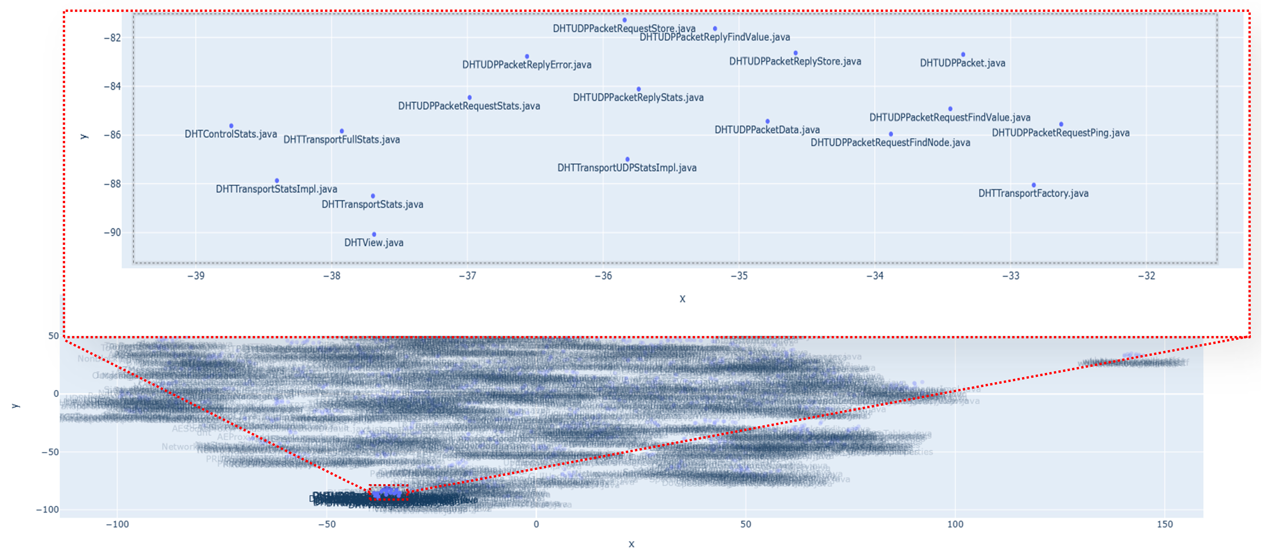
| Single input query “DHTUDPPacketRequest.java” | DHTUDPPacketRequestFindValue.java | 0.885 |
| DHTUDPPacketRequestPing.java | 0.870 | |
| DHTUDPPacketRequestFindNode.java | 0.869 | |
| DHTUDPPacketReply.java | 0.868 | |
| DHTUDPPacket.java | 0.867 | |
| DHTUDPPacketData.java | 0.862 | |
| DHTTransportUDP.java | 0.841 | |
| DHTUDPPacketRequestStore.java | 0.838 | |
| DHTTransportStatsImpl.java | 0.837 | |
| DHTUDPPacketReplyStats.java | 0.809 | |
| Group input query: [“DHTTransportUDP.java”, “DHTUDPPacketReply.java”, “DHTUDPPacketRequest.java”] | DHTUDPPacketRequestFindValue.java | 0.914 |
| DHTUDPPacketData.java | 0.910 | |
| DHTUDPPacket.java | 0.909 | |
| DHTUDPPacketReplyFindNode.java | 0.906 | |
| DHTUDPPacketReplyPing.java | 0.894 | |
| DHTUDPPacketRequestFindNode.java | 0.882 | |
| DHTUDPPacketRequestStore.java | 0.881 | |
| DHTUDPUtils.java | 0.880 | |
| DHTUDPPacketRequestPing.java | 0.876 | |
| DHTUDPPacketReplyStats.java | 0.871 | |
Disclaimer/Publisher’s Note: The statements, opinions and data contained in all publications are solely those of the individual author(s) and contributor(s) and not of MDPI and/or the editor(s). MDPI and/or the editor(s) disclaim responsibility for any injury to people or property resulting from any ideas, methods, instructions or products referred to in the content. |
© 2023 by the authors. Licensee MDPI, Basel, Switzerland. This article is an open access article distributed under the terms and conditions of the Creative Commons Attribution (CC BY) license (https://creativecommons.org/licenses/by/4.0/).
Share and Cite
Ahmed, H.A.; Lee, J. FCP2Vec: Deep Learning-Based Approach to Software Change Prediction by Learning Co-Changing Patterns from Changelogs. Appl. Sci. 2023, 13, 6453. https://doi.org/10.3390/app13116453
Ahmed HA, Lee J. FCP2Vec: Deep Learning-Based Approach to Software Change Prediction by Learning Co-Changing Patterns from Changelogs. Applied Sciences. 2023; 13(11):6453. https://doi.org/10.3390/app13116453
Chicago/Turabian StyleAhmed, Hamdi Abdurhman, and Jihwan Lee. 2023. "FCP2Vec: Deep Learning-Based Approach to Software Change Prediction by Learning Co-Changing Patterns from Changelogs" Applied Sciences 13, no. 11: 6453. https://doi.org/10.3390/app13116453