Scene Reconstruction Algorithm for Unstructured Weak-Texture Regions Based on Stereo Vision

Featured Application

The algorithms proposed in this paper can be applied to a wide range of infrastructure projects in the pre-survey process with the advantages of low cost and high practicality.

Abstract

At present, Chinese 3D reconstruction solutions using stereo cameras mainly face known, indoor, structured scenes; for the reconstruction of unstructured, larger-scale scenes with a large variety of texture information of different intensities, there are certain difficulties in ensuring accuracy and real-time processing. For the above problems, we propose a scene reconstruction method using stereo vision. Firstly, considering the influence of outdoor lighting and weather on the captured 2D images, the optimized SAD-FAST feature detection algorithm and stereo-matching strategy were employed in the stereo-matching stage to improve the overall efficiency and matching quality at this stage. Then, a homogenized feature extraction algorithm with gradient value decreasing step by step (GVDS) was used in the depth value calculation to ensure a sufficient number of feature points for strong texture information while extracting features from weak-texture areas, which greatly improved the quality and speed of unstructured scene reconstruction. We conducted experiments to validate the proposed method, and the results showed the feasibility of the proposed method and its high practical value.

1. Introduction

Vision-based 3D reconstruction technology is an important element of research in the computer field [1]. It works mainly through the use of relevant instruments to obtain two-dimensional image data information for objects. The acquired data information is then analyzed and processed and, finally, the theory of 3D reconstruction is used to reconstruct the contour information for the object surface in the real environment [2,3,4,5,6,7,8,9]. Vision-based 3D reconstruction technology has been widely used in the fields of unmanned vehicles [10], virtual reality [11], 3D printing [12], and engineering surveys [13].

At present, the 3D reconstruction methods for scenes are mainly divided into three categories [14]. The first type [15] involves the use of 3D laser scanning equipment to complete the 3D reconstruction, employing the optical principle to carry out optical scanning of the scene or object to obtain a high-accuracy 3D model. However, the reconstructed scene model has no texture, and the laser scanning equipment is expensive. The second type is the 3D reconstruction approach represented by the structure from motion method [16]. It only needs a monocular camera and the reconstruction cost is low [17], but the image acquisition and calculation require significant amounts of time [18] and the real-time performance is not good. The third type [19,20,21,22] is the 3D reconstruction method based on stereo vision. This method simulates the binocular imaging principle of human beings to obtain 3D information from the observed two-dimensional image information. It can be adapted to a variety of lighting environments; does not require too much human manipulation in use; can be employed for automatic, online, non-contact detection; has the advantages of adaptability, speed, high accuracy, low cost, etc. [6,23,24,25,26]; and can be successfully implemented for universal reconstruction projects.

Although 3D reconstruction technology based on stereo vision has many advantages, the traditional method still has disadvantages, such as redundant calculation of stereo matching, low real-time processing speed, and the scene information selection directly affecting the reconstruction effect. For example, Wang et al. [27] used an innovative MVS algorithm for the surface reconstruction task that employs planar patches of different scales to fit the surface and can yield a visualized 3D model with high accuracy. However, this method is built on the need for multiple views of the target to be reconstructed and a small target class, which makes it difficult to obtain better real-time processing and applicability. Furukawa et al. [28] divided input stereo images into clusters with small overlaps to alleviate the scalability problem affecting large numbers of images in the feature-growth method, but their computational complexity remains the primary problem in scene reconstruction. Mnich [29] attempted to reconstruct the GMAW pool using a stereo-vision approach, but the significant effect of light intensity on the reconstruction quality suggested that the stereo reconstruction system could be improved. Liang et al. [30] established a two-prism stereo-vision system and proposed a two-step stereo-matching algorithm to reconstruct the surface 3D shape, but since some areas on reconstructed surfaces are discontinuous, it cannot be applied to our reconstruction of unstructured scenes. Considering the popularity of deep learning in recent years, Yang and Jiang [31] combined deep learning algorithms with traditional algorithms to extract and match feature points from optical pattern-enhanced images to improve practical 3D reconstruction methods for weakly textured scenes. Stathopoulou et al. [32] solved the texture-free problem by exploiting semantic priors for the PatchMatch-based MVS to increase confidence and better support depth and normal mapping estimation in weakly textured regions. However, even with the combination of these traditional algorithms and deep learning, visual reconstruction of unstructured building surfaces or large, weakly textured areas commonly found in cities remains a challenge.

Of course, when dealing with reconstruction tasks involving weakly textured or even non-textured objects, the use of photometric 3D reconstruction-related theories is usually effective. Generally, photometric 3D reconstruction can be broadly classified into two types: shape from shading (SFS) and photometric stereo (PS). Both types are based on the assumption that the reflective properties of the object surface follow the Lambert reflective film properties. When the camera follows the orthogonal projection conditions, these two types of reconstruction problems can be essentially solved with the image irradiance equation [33]. The image irradiance equation is shown below.

$$I\left(x,y\right)=R\left(n\left(x,y\right)\right)=R\left(p\left(x,y\right),q\left(x,y\right)\right)$$

(1)

where $I\left(x,y\right)$ is the grayscale value of the image observed by the camera and $R\left(p,q\right)$ is the reflectance map determined by the reflectance model. At this point, according to the photometric theory, the reflection diagram $R\left(p,q\right)$ is

$$R\left(p,q\right)=\rho \left(x,y\right)\cos {\theta }_i$$

(2)

where $\rho \left(x,y\right)$ is the reflectance of the Lambert object surface $z=z\left(x,y\right)$.

$$\cos {\theta }_i=\frac{n}{\Vert n\Vert }•\frac{L}{\Vert L\Vert }=\frac{p_{s}p+q_{s}q+1}{\sqrt{p_s^2+q_s^2+1}\sqrt{p^2+q^2+1}}$$

(3)

Substituting Equations (2) and (3) into Equation (1), the SFS image irradiance equation can be obtained.

$$I\left(x,y\right)=\rho (x,y)\frac{p_{s}p\left(x,y\right)+q_{s}q\left(x,y\right)+1}{\sqrt{p_s^2+q_s^2+1}\sqrt{p^2\left(x,y\right)+q^2\left(x,y\right)+1}}$$

(4)

However, it is also clear that, for the image irradiance (Equation (4)), there are three unknowns: $\rho (x,y)$, $p\left(x,y\right)$, and $q\left(x,y\right)$. One of the most straightforward approaches is to remove the issue by increasing the illumination constraints. In other words, in order to determine these three unknown quantities, at least three uncorrelated image irradiance equations need to be constructed, which is exactly the research idea proposed by Woodham [34], who developed the photometric stereo 3D reconstruction method. He proposed a photometric stereo method, as shown in Figure 1b, using $m\left(m\ge 3\right)$ light sources $L_1,L_2,\dots ,L_m$ in different directions to sequentially illuminate the same object under scrutiny and obtain $m$ images. The $I_1\left(x,y\right),I_2(x,y),\dots ,I_m(x,y)$ equations can be combined to obtain:

$$\{\begin{array}{l}{I}_1\left(x,y\right)=\rho (x,y)\frac{p_{s1}p(x,y)+q_{s1}q(x,y)+1}{\sqrt{p_{s1}^2+q_{s1}^2+1}\sqrt{p^2(x,y)+q^2(x,y)+1}}\\ I_2\left(x,y\right)=\rho (x,y)\frac{p_{s2}p(x,y)+q_{s2}q(x,y)+1}{\sqrt{p_{s2}^2+q_{s2}^2+1}\sqrt{p^2(x,y)+q^2(x,y)+1}}\\ \hspace{1em}\hspace{1em}\hspace{1em}\dots \\ I_m\left(x,y\right)=\rho (x,y)\frac{p_{sm}p(x,y)+q_{sm}q(x,y)+1}{\sqrt{p_{sm}^2+q_{sm}^2+1}\sqrt{p^2(x,y)+q^2(x,y)+1}}\end{array}$$

(5)

For the convenience of calculation, note that the light unit direction vector is $S_i=L_i/\Vert L_i\Vert$, the unit normal vectors on the surface of the object are $N(x,y)=n(x,y)/\Vert n(x,y)\Vert$ and $g(x,y)=\rho (x,y)N(x,y)$, and the system of irradiance equations for photometric stereo images is obtained by collating the above equations.

$$\{\begin{array}{l}{I}_1(x,y)=g(x,y)\cdot S_1\\ I_2(x,y)=g(x,y)\cdot S_2\\ \hspace{1em}\hspace{1em}\hspace{1em}\dots \\ I_m(x,y)=g(x,y)\cdot S_m\end{array}\triangleq i(x,y)=Sg(x,y)$$

(6)

In the formula, $i(x,y)={(I_1(x,y),I_2(x,y),\dots ,I_m(x,y))}^T, S={(S_1^T,S_2^T,\dots ,S_m^T)}^T$. Obviously, $g\left(x,y\right)$ can be obtained by solving the linear system in Equation (6). Typically, when $m\ge 4$, the least-squares solution (Equation (7)) for the linear system in Equation (6) can be calculated and then $\rho (x,y),N(x,y)$ can be reconstructed.

$$g(x,y)={(S^{T}S)}^{-1}{S}^{T}i(x,y)$$

(7)

$$\rho (x,y)=\Vert g(x,y)\Vert$$

(8)

$$N(x,y)=\frac{g(x,y)}{\rho (x,y)}=\frac{g(x,y)}{\Vert g(x,y)\Vert }$$

(9)

Further, if the 3D morphology $z(x,y)$ of the object surface needs to be reconstructed, it this can be achieved by integrating the normal vector $N(x,y)$. The specific integration method can be found in the literature [35,36,37,38,39,40]. However, photometric stereo reconstruction is often applied in the field of defect detection, where the object is usually an object that can move rather than a scene, and the method requires more pre-processing steps to carry out experiments, which has a greater impact on the real-time processing.

Aiming at the defects and deficiencies of these existing 3D reconstruction techniques based on stereo vision, we propose a scene reconstruction method with better accuracy and real-time performance. Our contributions can be summarized as follows:

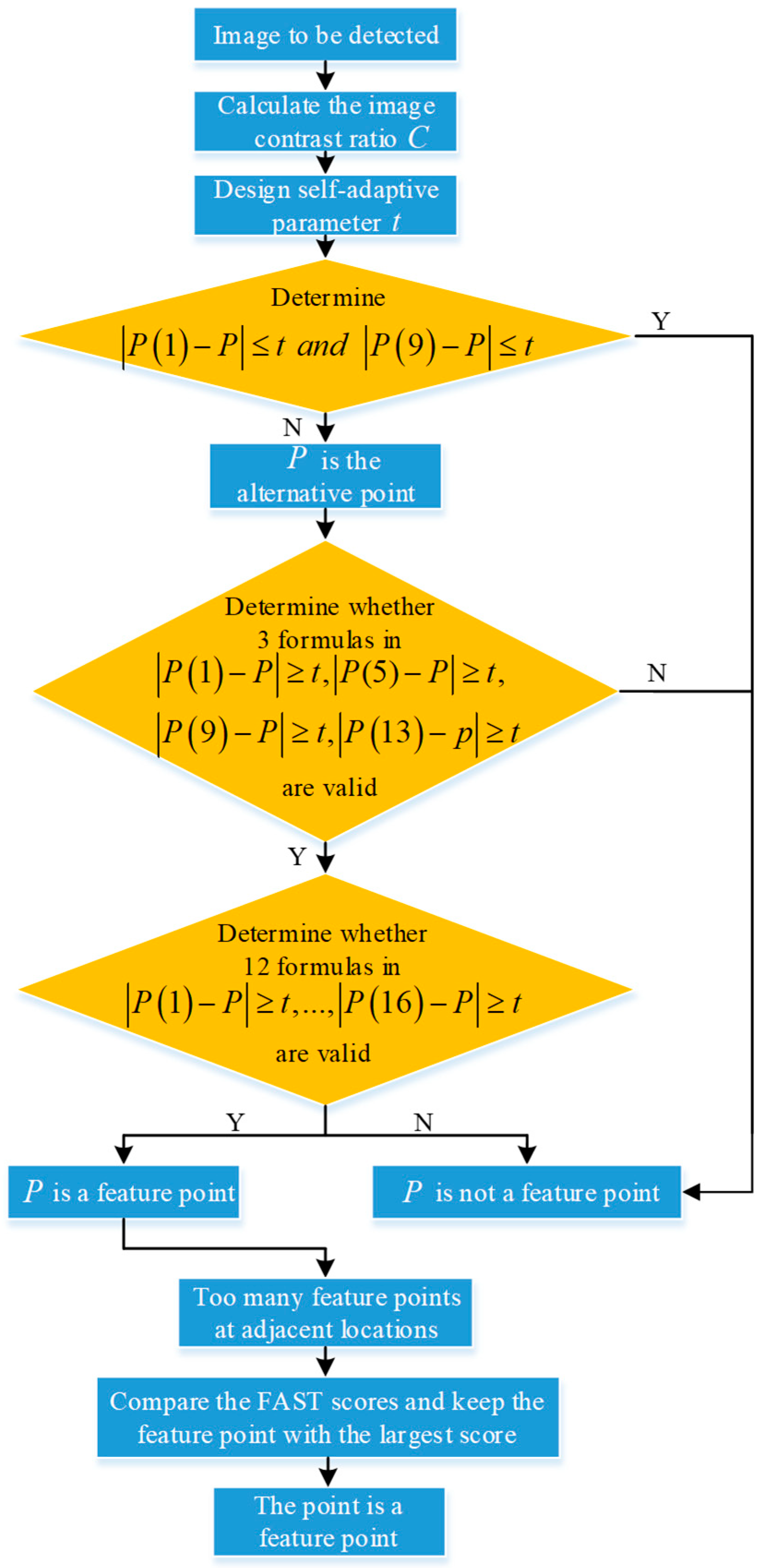
• Based on the FAST feature detection algorithm, a SAD-FAST feature detection algorithm with newer and smarter decision conditions is proposed. This algorithm changes the fixed grayscale difference threshold used by the traditional FAST detection into a self-adaptive grayscale difference threshold based on the light and dark stretch contrast of the image to avoid missing the necessary feature points and improves the feature point judgment conditions to screen the feature points with higher quality;
• In this study, the three-step correlation algorithm in the stereo-matching system based on feature points was adopted to “select the essence and discard the dross”, and a combination method of FAST feature detection + SURF feature description + FLANN feature matching is proposed. Furthermore, the Mahalanobis distance was used to reduce the mismatching between different dimensions when matching, which ensured efficiency and accuracy when facing complex texture scenes. We propose a GVDS feature extraction algorithm to adjust the distribution of feature points, avoiding the loss of 3D information caused by the absence of feature points in part of the scene to be reconstructed and thus making the final reconstruction effect more realistic and improving the reconstruction efficiency.

As can be seen, our proposed algorithms focus on the two most critical steps (stereo matching and depth value calculation) in stereo 3D reconstruction. The SAD-FAST feature detection algorithm can perfectly solve the problem that feature points are difficult to detect in weak-texture regions and can find the feature points with the strongest feature information in a certain region to solve the problem of overly dense distribution. The improved stereo-matching system had a significantly improved matching success rate and real-time performance compared to the inherent system, and it finally yielded disparity maps with good disparity in weakly textured regions without the help of hole filling or filter denoising. In the depth value calculation, our proposed GVDS algorithm could effectively avoid the loss of 3D information in weakly textured regions without neglecting the key points in regions with strong depth variations, making it possible to derive complete 3D point-cloud maps, which are irreplaceable for the generation of the final complete models. We took pictures with the stereo camera platform that we built for experimental evaluation. The experimental results showed that the proposed algorithm has strong real-time performance and robustness, and the reconstruction effect was good.

2. Stereo Reconstruction Algorithm for Unstructured Scenes

Three-dimensional scene reconstruction is a process of obtaining 3D information for an actual scene and finally producing a visual model according to the 2D information from the image shot by the relevant camera [41]. Using a stereo-vision system to complete 3D reconstruction is the key and difficult point in today’s 3D reconstruction systems [42]. As shown in Figure 2, 3D reconstruction with stereo vision was achieved through steps such as stereo matching, depth value calculation, triangulation, and texture mapping.

Stereo matching refers to establishing the corresponding relation between a pair of images according to the extracted features; that is, mapping the same physical space points in two different images one by one [43,44,45]. Image preprocessing is required before stereo matching [46].

Depth value calculation [47] refers to the process of reconstructing the 3D point cloud for the scene using the camera model and the disparity map and is divided into two parts: selecting the corresponding feature points and calculating the 3D coordinates.

The ultimate goal of 3D reconstruction is to visually display the reconstructed model, and triangulation is equivalent to building a 3D mesh skeleton model for the scattered 3D point set [48].

Texture mapping [49,50,51] refers to extracting the texture of a scene from a 2D image and mapping it onto a mesh skeleton to obtain a realistic 3D model of the scene.

2.1. SAD-FAST Feature Detection and Recombination Stereo-Matching System

As the most critical step in stereo 3D reconstruction technology, the commonly used algorithms are divided into the following broad categories: matching based on regions, matching based on phases, and matching based on feature points. Region matching uses feature vectors for matching, and it is computationally intensive, inefficient, and prone to mismatching. Phase matching is based on the assumption that the local phases between the corresponding pixels of two corresponding images should be equal and has a low bit error rate, but phase deviation has a huge impact on the matching accuracy. Feature matching is currently the most researched algorithm in the field of stereo matching and is based on special pixel points, such as corner points and edges. It has the advantages of low computation requirements, strong stability, and high real-time efficiency, and the probability of such feature points disappearing over time is very small, so the feature matching algorithm can basically meet the needs of 3D reconstruction projects.

The algorithm for matching based on feature points can be divided into the following three steps, as shown in Figure 3: feature detection, feature description, and feature matching.

In recent decades, research scholars have not stopped studying feature detection algorithms, and many algorithms with excellent performance have emerged, such as AKAZE, FREAK, and BRISK, which focus on corner point detection; the Harris and features from accelerated segment (FAST) algorithms, which have been the most commonly used in recent years; and SIFT, SURF, and ORB. Considering the uncertainty regarding the strength of the texture information in different regions of unstructured, outdoor scenes, we propose a combination of FAST feature detection + SURF feature description + a FLANN matcher for stereo matching under the general framework of the existing stereo-matching algorithms based on feature points for the sake of both matching accuracy and effectiveness, and we used the Mahalanobis distance instead of the Euclidean distance to determine the matching degree. For the contrast uncertainty affecting illumination and environmental information, an improved SAD-FAST feature detection method is proposed that uses the contrast of the image to adaptively adjust the threshold value during feature point detection and resets the process of determining feature points, solving the problem of too many feature points being adjacent to each other.

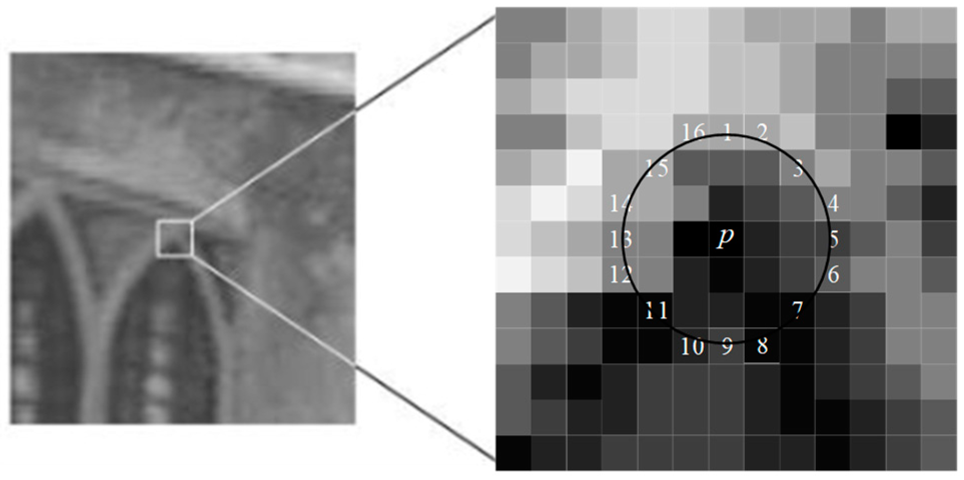
2.1.1. SAD-FAST Feature Detection

The FAST feature detection algorithm was proposed by Rosten in 2006 and is one of the currently accepted fast corner-point detection algorithms. The FAST feature detection algorithm determines whether a pixel is a feature by comparing the magnitude of the gray value of the pixel with those of its surrounding neighborhood and characterizes the feature orientation by determining the gray gradient around the feature. This process is simple, easy to implement, and efficient. However, in the actual environment, due to the uncertainty of light and surrounding environment information, it is very easy for a sharp decrease in the number of feature points to occur when the environmental contrast ratio decreases. Based on the above, we propose a self-adaptive threshold value method for SAD-FAST feature detection.

When using conventional FAST for feature point detection, the grayscale difference threshold used is artificially set. When the light intensity and the surrounding environment’s contrast ratio changes, the number of detected feature points will be reduced, which can easily lead to inaccurate experiments and other results. Based on the above problems, we propose a self-adaptive threshold value calculation method. Firstly, we calculate the image contrast ratio; i.e., the degree of stretching contrast between light and dark.

$$C={\displaystyle \sum _{\delta }\delta {\left(i,j\right)}^2{P}_{\delta }\left(i,j\right)}$$

(10)

where $\delta \left(i,j\right)=\left|i-j\right|$ is the grayscale difference between adjacent pixels. $P_{\delta }(i,j)$ is the probability of a pixel distribution with a grayscale difference of $\delta$ between adjacent pixels. Based on the derived image contrast ratio $C$, the self-adaptive threshold value $t$ can be designed with the formula:

$$t=\alpha C$$

(11)

where $\alpha$ is the self-adaptive parameter, and the value is determined according to the experimental data.

As shown in Figure 4, let the point to be detected be $P$, with $P$ being the center of a circle and three pixel points as the radius forming a circle field. Take 16 pixel points on the edge of the circle, set the grayscale threshold $t>0$, and compare the magnitude of the grayscale value $I\left(x\right)$ of each pixel point $x$ on the circle with the grayscale value $I\left(P\right)$ of $P$. It is easy to see that three cases can occur:

• $I\left(x\right)-I\left(P\right)>t$, and point $x$ is brighter than point $P$;
• $I\left(P\right)-I\left(x\right)>t$, and point $x$ is darker than point $P$;
• $-t\le I\left(x\right)-I\left(P\right)\le t$, and the two points are of equal brightness.

Although a large number of non-angular regions can be eliminated with the traditional FAST detection algorithm, there are still several obvious shortcomings. First, in the pixel test of 16 surrounding pixel points, the traditional FAST algorithm only considers the pixel difference or brightness degree of 4 pixel points to determine whether a point should be classified as a corner point, without more stringent screening. Second, the choice of pixels is not exactly optimal. Third, multiple features are easily detected in close proximity to each other. To address the above issues, we improved the feature determination of FAST.

First, define a threshold value. The pixel difference between $P\left(1\right)$, $P\left(9\right)$, and the center $P$ are then calculated. If their absolute values are less than the threshold, the point $P$ cannot be a feature point; otherwise, it is classified as an alternative point for the next step.

If point $P$ is an alternative point, the pixel differences between $P\left(1\right)$, $P\left(9\right)$, $P\left(5\right)$, $P\left(13\right)$, and the center $P$ are calculated, and if at least three of their absolute values exceed the threshold, then point $P$ is classified as an alternative point; otherwise, it is not.

If point $P$ is an alternative point, the pixel difference between a total of 16 points from $P\left(1\right)$ to $P\left(16\right)$ and the center $P$ is calculated, and if at least 12 of them exceed the threshold, then $P$ is determined to be the alternative point.

When multiple alternative points are detected at adjacent locations, we can use non-maximum suppression to solve the selection problem. First, the FAST score value is calculated with the feature points, and if there are multiple feature points in a neighborhood centered on the feature point $P$, the score value of each feature point is judged (the sum of the absolute values of the differences between each of the 16 points and the center point). If $P$ is the largest among all feature points in the neighborhood, it is retained; otherwise, it is not.

The overall process of the improved SAD-FAST detection algorithm is shown in Figure 5.

2.1.2. SURF Descriptor

The SURF algorithm stands out for its good rotational and fuzzy robustness. After the feature corner points have been pinpointed by the SAD-FAST algorithm, our idea was to use these feature corner points to replace the scale- and selection-invariant feature points already identified by Hessian detector in the SURF algorithm. Before performing feature matching with image pairs, the position and orientation information for feature corner points needs to be computed to obtain and then generate the required 64-dimensional feature descriptors.

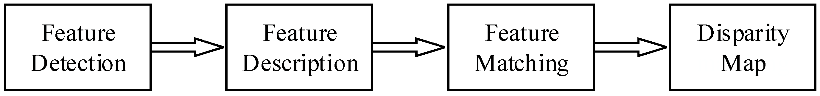
2.1.3. FLANN Feature Matching

The FLANN feature matching algorithm was proposed in 2009 by Muja et al. [52] It implements a collection of search algorithms, including KD-TREE, which is the most complete open-source library of nearest neighbors available. For the SURF descriptor used in our experiments, the FLANN matcher used the Euclidean distance to find the nearest neighbors of the instances because of its float descriptor nature.

2.1.4. Mahalanobis Distance

Euclidean distance treats the differences between different dimensions as equivalent, which is very likely to lead to mismatching of feature points. The Mahalanobis distance corrects this shortcoming by considering the relationship between various characteristics. In addition, cross-matching was added to the calculation, for which it is commonly understood that, after a feature point in the matching image searches for a corresponding point in the image to be matched, the corresponding point returns to search for a feature point in the matching image, and the two points derived from the two processes are observed to see if they correspond; if so, they are regarded as a pair of matching points. The formula for calculating the Mahalanobis distance between two feature points $X$ and $Y$ is shown below.

$$D_{(x,y)}=\sqrt{{(X-Y)}^T{S}^{-1}(X-Y)}$$

(12)

$$S=\mathrm{cov}(X,Y)=E\left\{\left[X-E\left(X\right)\right]\left[Y-E\left(Y\right)\right]\right\}$$

(13)

where $S$ is the covariance matrix of the two feature points and $E$ is the mean value. When the covariance is the identity matrix—that is, each dimension is independently distributed—the Mahalanobis distance becomes the Euclidean distance. The method substantially reduces the risk of mismatching and demonstrates a good matching effect and real-time performance with only a subtle increase in the number of operations.

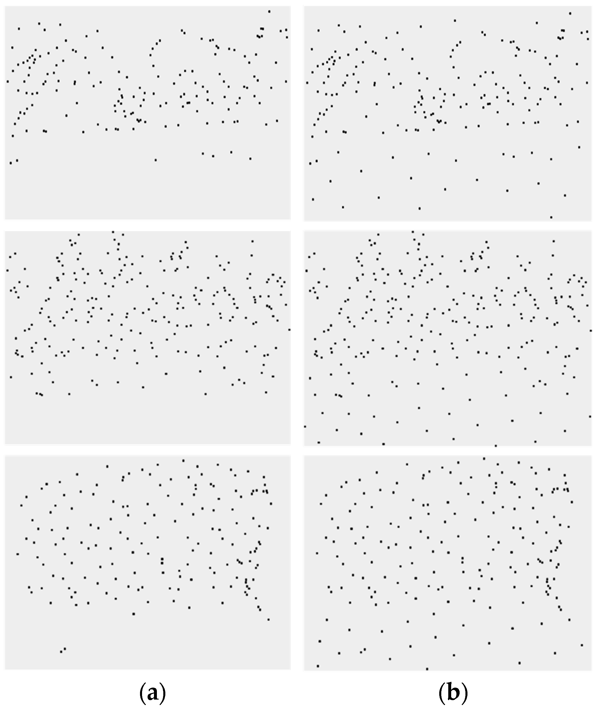
2.2. GVDS Feature Extraction Algorithm

The calculation of the depth value is the process of finding the set of spatial 3D points and includes two parts: the selection of feature points and the calculation of the depth value. When conducting a stereo 3D reconstruction project, the stereo camera can generally use a fixed camera position and parallel structure pose to shoot the scene to be reconstructed. The schematic diagram of the depth value calculation with the stereo parallel optical axis structure is shown in Figure 6.

As shown in Figure 6, point $P\left(X_w,Y_w,Z_w\right)$ is an observed point in 3D space that corresponds to points $P\left(u_l,v_l\right)$ and $P\left(u_r,v_r\right)$ on the imaging planes of the left and right cameras, respectively, and points $O_{CL}$ and $O_{CR}$ indicate the optical centers of the left and right cameras, respectively. It is obvious from observation that the relationship between these five points in space is in accordance with the triangulation principle.

Since the main ray axes of the left and right cameras are horizontal and parallel, the x-axes of the coordinate systems of the two cameras overlap; that is, disparity only exists in the direction of $x$. The formula for calculating disparity $d$ is:

$$d=L_l-L_r$$

(14)

According to Figure 6, using the similar triangle determination property, we can conclude that:

$$\frac{f}{Z_w}=\frac{L_l}{B/2+X_w}=\frac{L_r}{B/2-X_w}$$

(15)

Combining the above two equations, the depth value $z$ of point $P$ can be expressed as:

$$z=\frac{B•f}{L_l-L_r}=\frac{B•f}{d}$$

(16)

Combined with the depth calculation formula, the depth information for point $P$ can finally be determined as follows:

$$\{\begin{array}{l}{X}_w=\frac{B•u_l}{u_r-u_l}\\ Y_w=\frac{B•u_l}{v_r-v_l}\\ X_w=\frac{B•f}{u_r-u_l}\end{array}$$

(17)

where $f$ is the camera focal length, $B$ indicates the distance between the left and right camera optical centers, and $d$ is the disparity value. The formula shows that the depth information for the object can be determined with only the corresponding point positions of the spatial points on the left and right images when the relevant parameters of the camera are known.

The above solution process can accurately obtain the 3D coordinates of a point in space. In order to reach the accuracy and efficiency required for scene reconstruction, it is necessary to first consider the distribution of the extracted feature point set and then calculate the 3D coordinates of the feature points. However, it is difficult to reconstruct the scene with weak texture information because this area contains very little information compared to the surrounding scene, and it is extremely difficult to guarantee the reconstruction quality while ensuring scene reconstruction efficiency. In the usual, fixed depth value calculation step, the feature points are extracted mechanically only in the areas with strong texture information and depth variation, and it is extremely difficult to extract feature points in the weak-texture and low-comparison areas with the same scene background. When faced with a scene that itself occupies a large number of weakly textured areas, the difficulty of extracting feature points can be the primary problem that prevents the formation of an effective visual 3D model.

To meet the dual criteria of accuracy and efficiency, it is necessary to consider the distribution of extracted feature points and then calculate the 3D coordinates of feature points to form a more efficient 3D point cloud. The distribution of feature points is closely related to the environment to be reconstructed, and unstructured scenes are often in natural environments with different distributions and intensities of texture information, which can easily lead to too dense or sparse a distribution of feature points, and this can affect the accuracy of subsequent texture mapping. Therefore, the distribution of the extracted feature points should be focused on before the depth values are calculated.

First, the feature points should be extracted in the region where the depth information varies widely; that is, the feature points of excellent quality should be selected.

Second, the distribution of feature points should not be too dense.

Third, some feature points should also be extracted from the regions with weak depth variation.

Based on the above idea, we propose a homogenized feature extraction algorithm with gradient value decreasing step by step (GVDS), and the calculation steps for this algorithm are as follows:

(1)

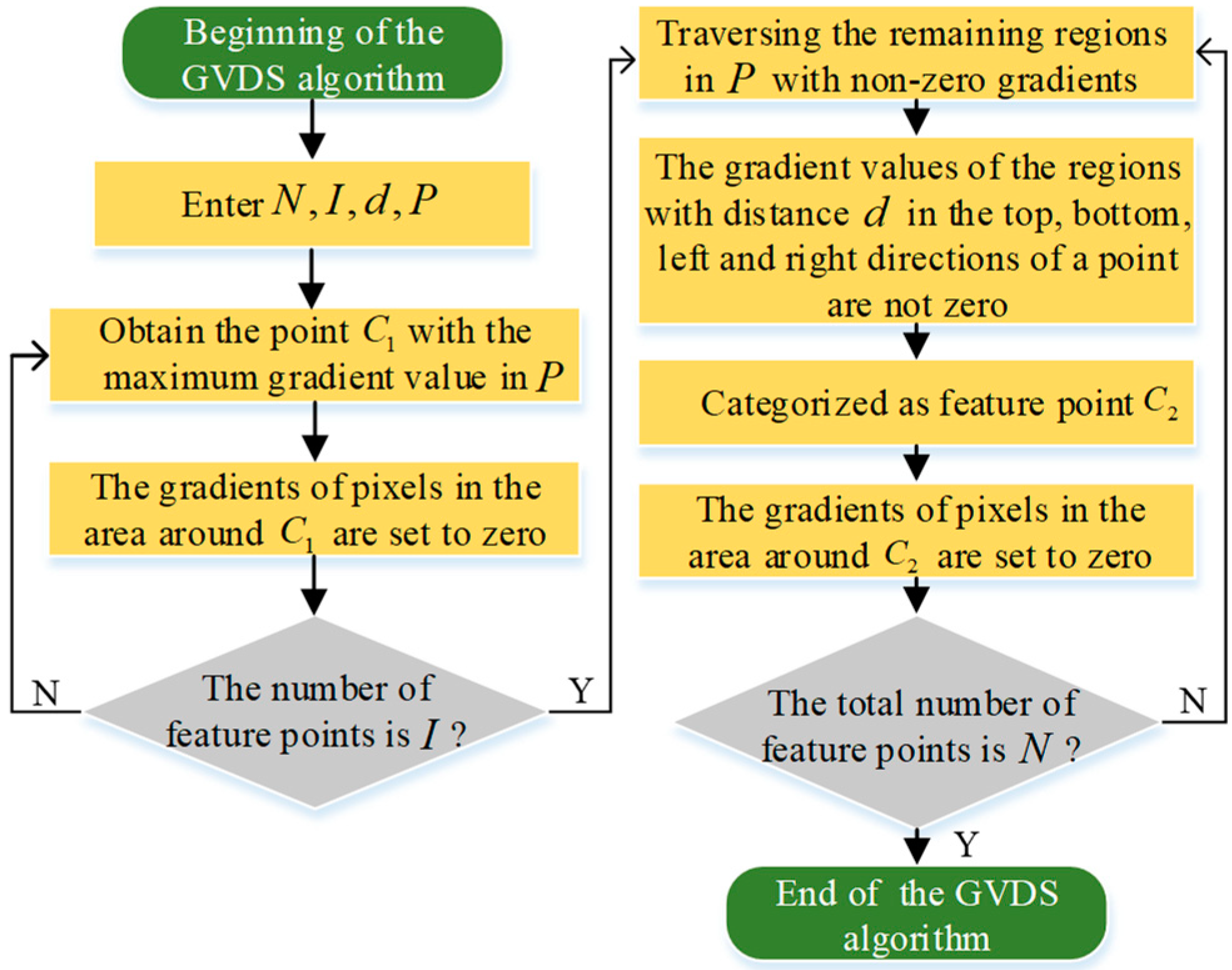
Set the total number of feature extraction points as $N$, the number of feature points with strong depth variation as $I$, the shortest Euclidean distance between adjacent feature points as $d$, and the disparity map derived from stereo matching as $P$;

(2)

Calculate the gradient value for the disparity map $P$, and then the point $C_1$ with the largest gradient value can be found, which is the first feature point selected;

(3)

In order to avoid too dense a distribution of feature points, the gradient of the surrounding pixels within a certain range should be set to zero after a feature point is selected. In the disparity map $P$, the gradient-zeroing operation is carried out in the surrounding area with point $C_1$ as the center of the circle and $d$ as the radius;

(4)

Repeat steps (2) and (3) until the number of selected feature points is not less than $I$;

(5)

Feature point extraction is performed for the remaining scattered regions with low depth variation in the disparity map $P$. A pixel coordinate in the disparity map $P$ is defined as $\left(d,d\right)$ so that it traverses the region with a non-zero gradient value starting from the top left of the disparity map $P$. If the gradient values of the pixels with distances of $d$ in the top, bottom, left, and right directions are not zero when the traversal reaches a certain point, the point is selected as the feature point and is called $C_2$;

(6)

The gradient of the surrounding area with point $C_2$ as the center and $d$ as the radius is set to zero;

(7)

Repeat steps (5) and (6) until the total number of feature points that have been selected is $N$.

The schematic diagram for the GVDS algorithm is shown in Figure 7. In order to obtain a better reconstruction effect, the GVDS feature extraction algorithm considers that the feature points are best taken in regions with strong depth variations, and the gradient-zeroing operation also avoids a dense distribution of feature points, while some feature points are further extracted in flat regions with weak depth variations.

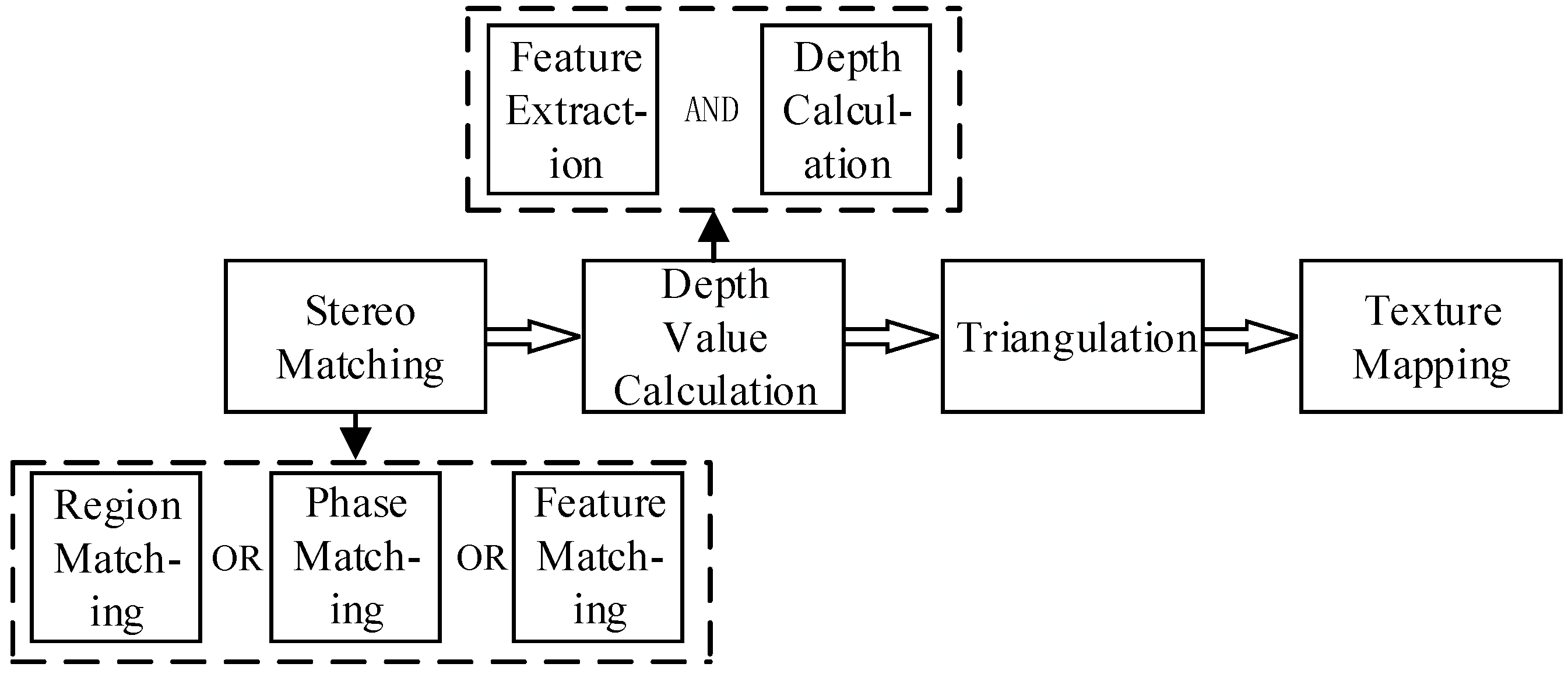
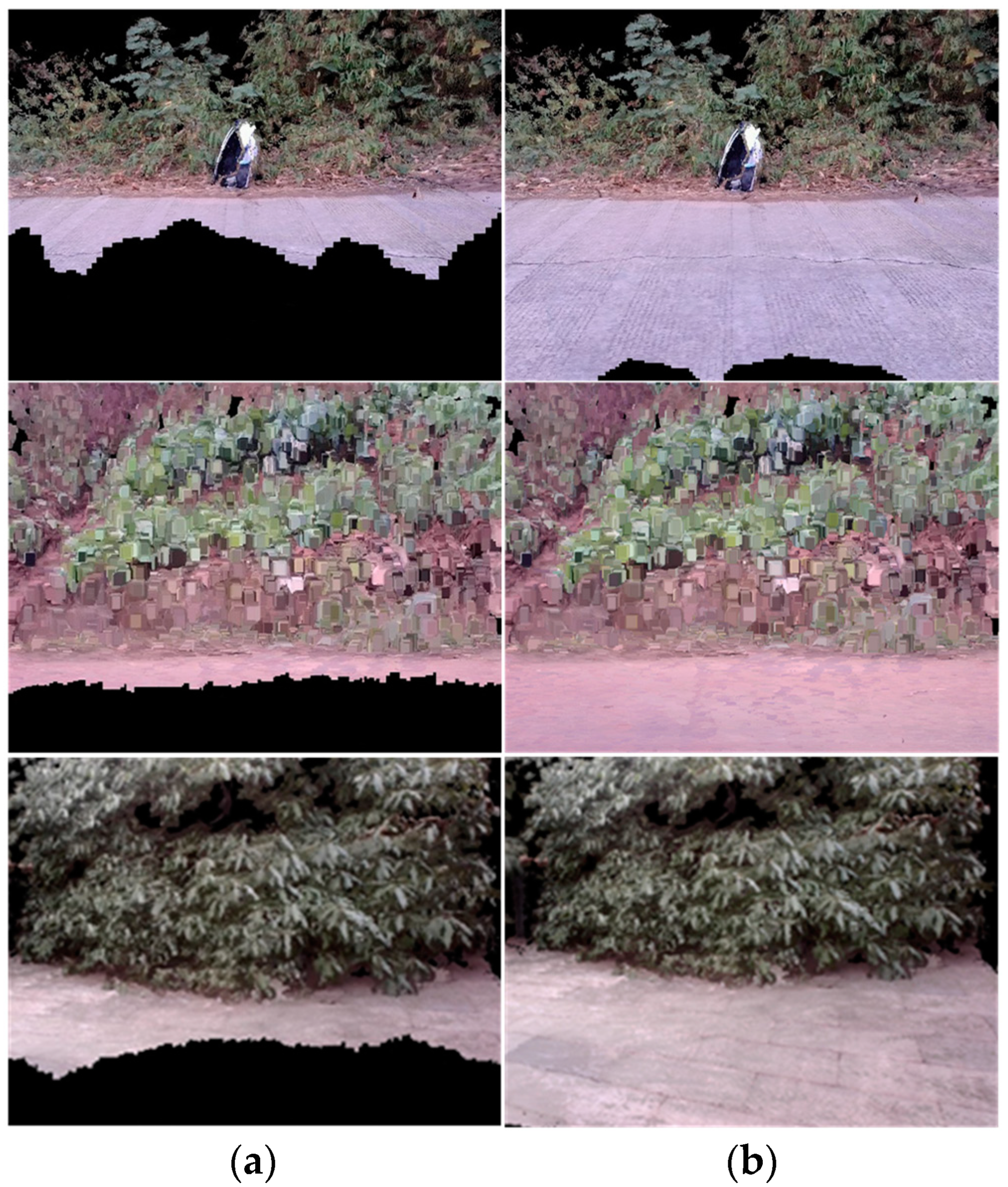
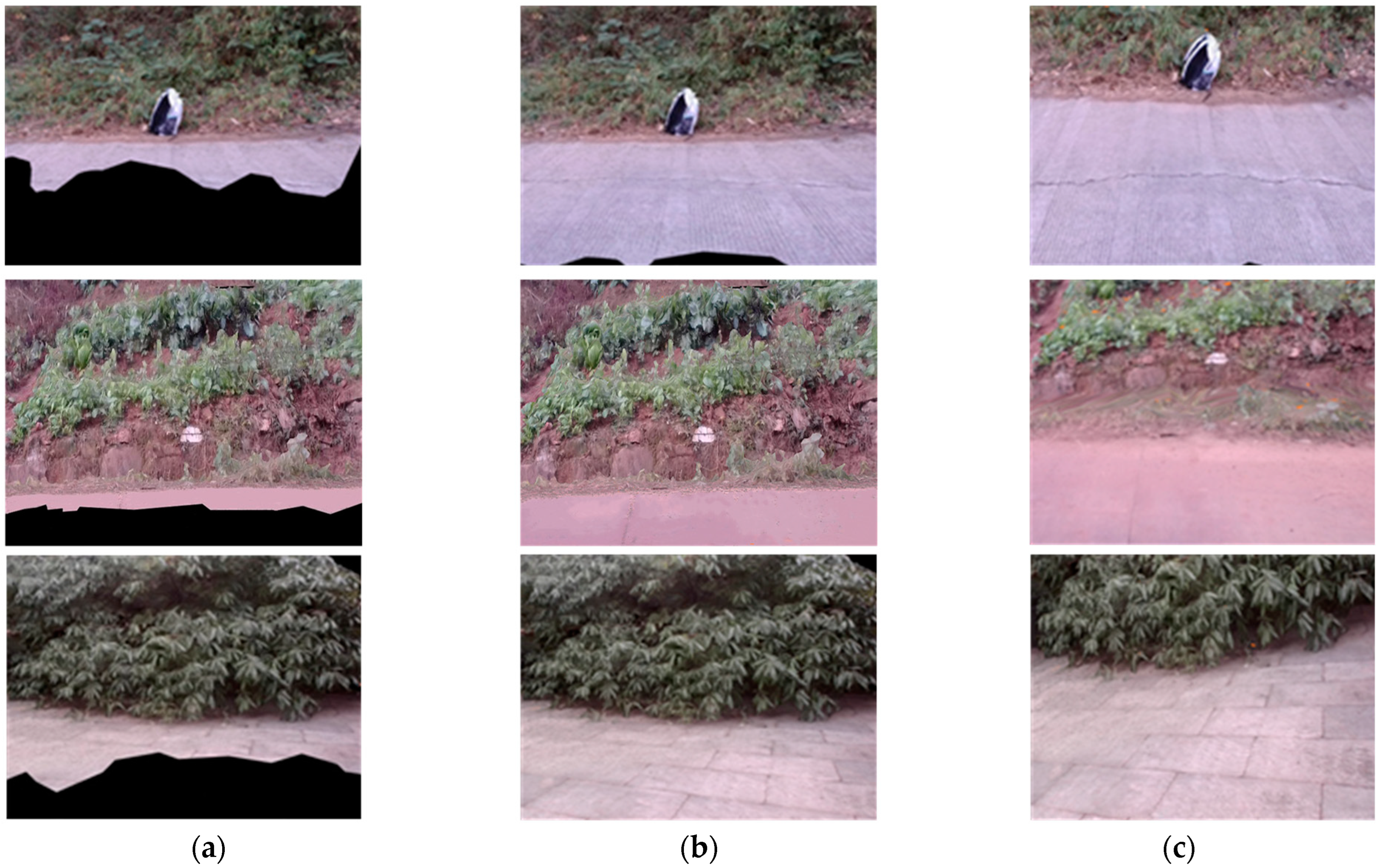
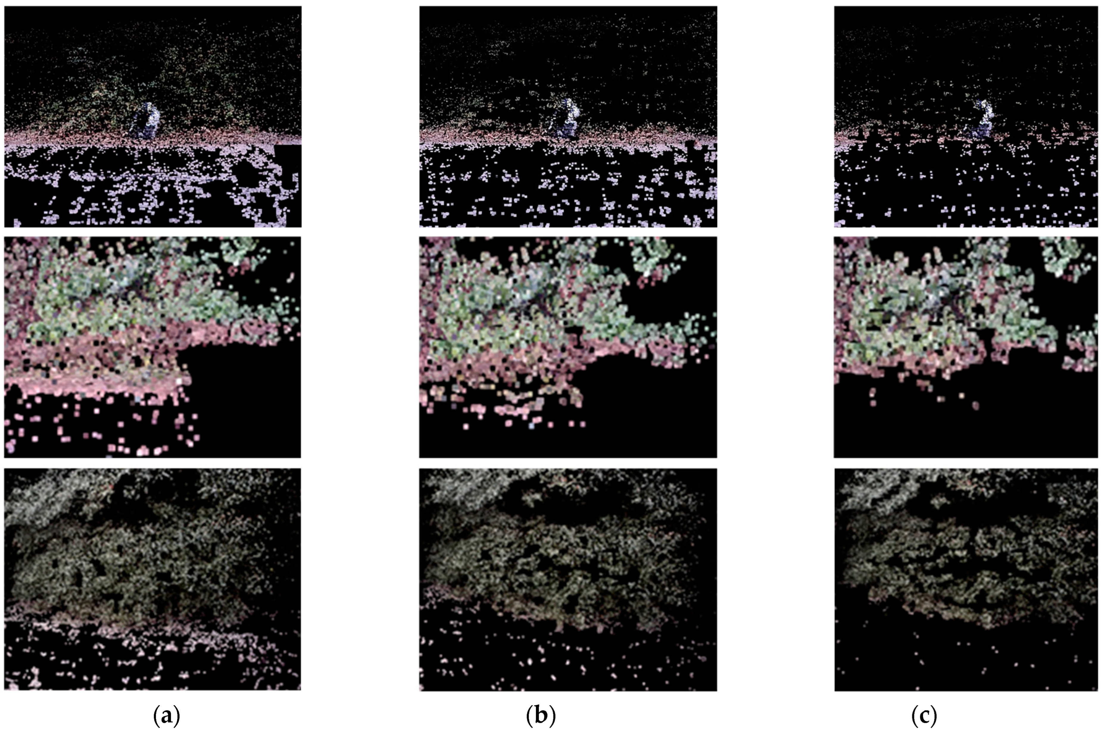
2.3. Triangulation and Texture Mapping

After calculating the spatial information for the feature points by calculating the depth value, these feature points are scattered in the three-dimensional space. If we want to complete the reconstruction of the three-dimensional scene, we also need to build these scattered three-dimensional points into a three-dimensional mesh skeleton model. Considering that the $x$ and $y$ projections of some of the point cloud data in the $xyz$ coordinate system overlapped, we combined the Delaunay triangulation algorithm with the idea of a partitioning algorithm to perform region segmentation, triangulate each subset of points according to the Delaunay triangulation algorithm, and, finally, merge each subset of points to triangulate the boundary of the subset of points.

Texture mapping is the process of mapping the 2D pixel coordinates of an image to spatial 3D coordinates. The three-dimensional mesh skeleton model formed with triangulation cannot yet make the objects in the scene feel realistic or achieve a realistic display of the scene. Texture mapping extracts the texture from the 2D image and maps it onto the stereo mesh skeleton model to recover the real texture of the surface and provide a realistic 3D model of the scene.

3. Experimental Results and Analysis

In our experiments, a four-megapixel camera was used to build a stereo experimental platform for outdoor scenes. The distance between the left and right cameras was set to 12 cm, and the images used in our experiments were taken from our stereo camera platform. The experimental platform used PyCharm and Microsoft Visual Studio 2017, the computer operating system was Windows 10, and the graphics card was an NVIDIA TITAN XP model with 12G of video memory. The stereo experimental platform is shown in Figure 8.

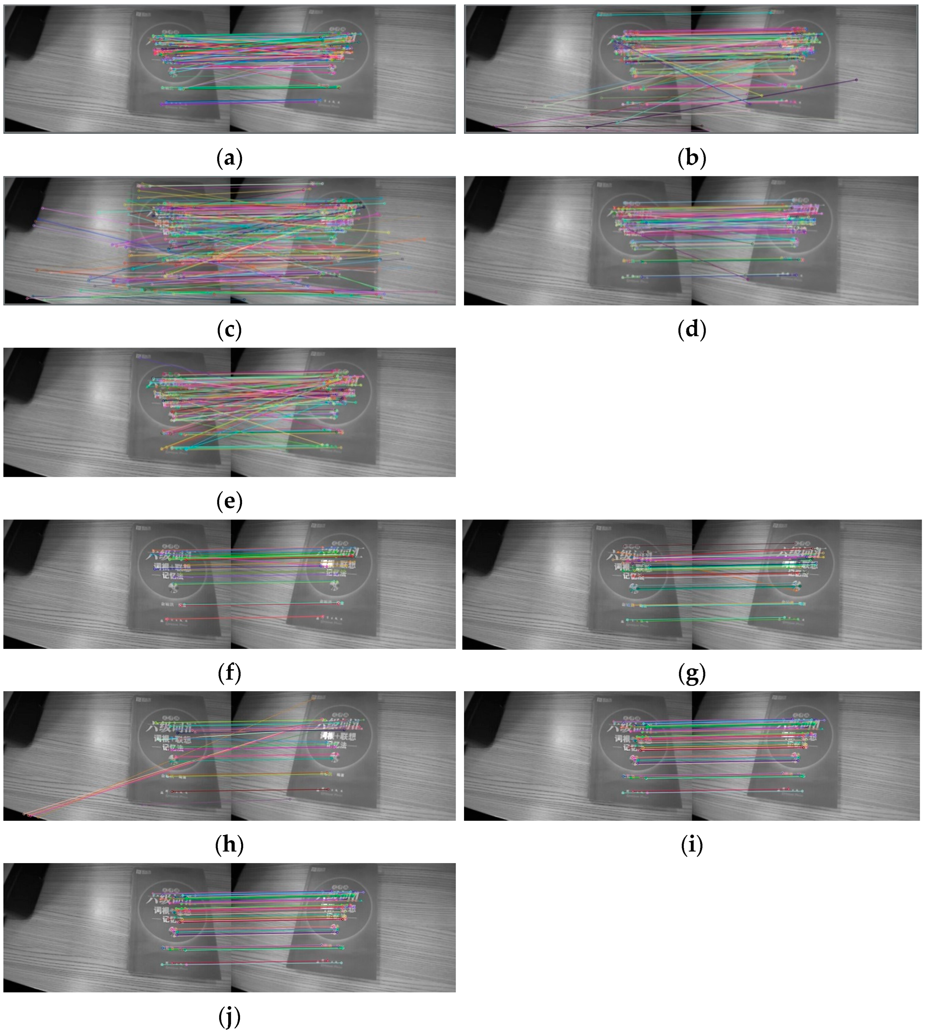
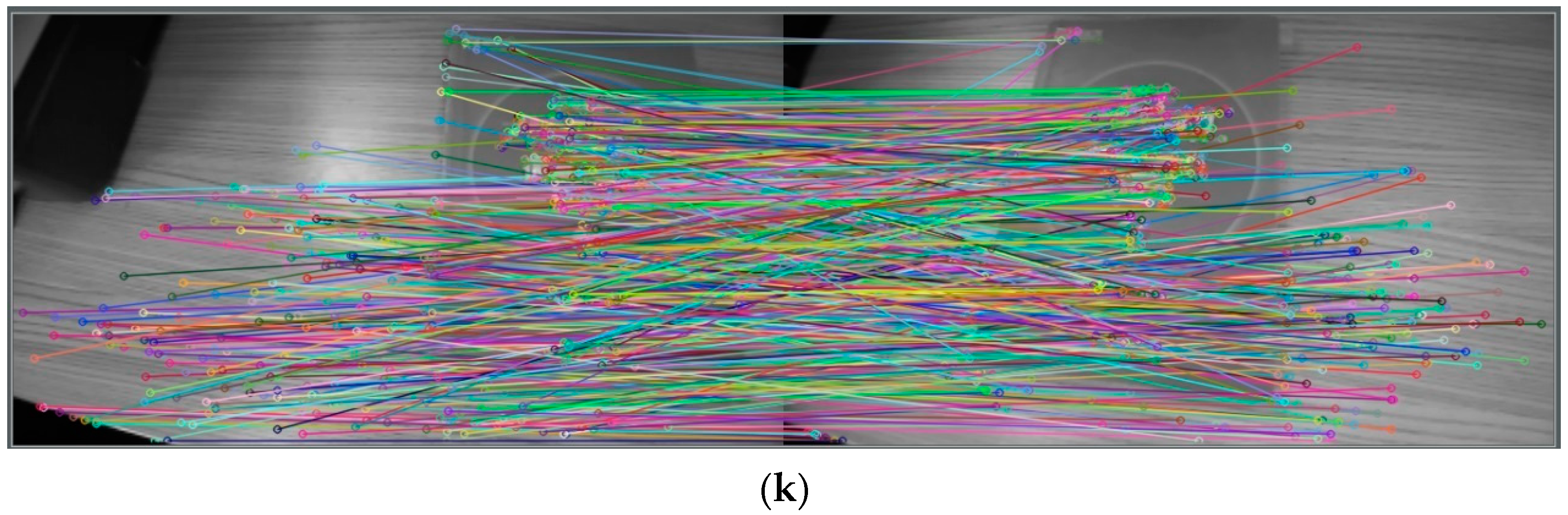
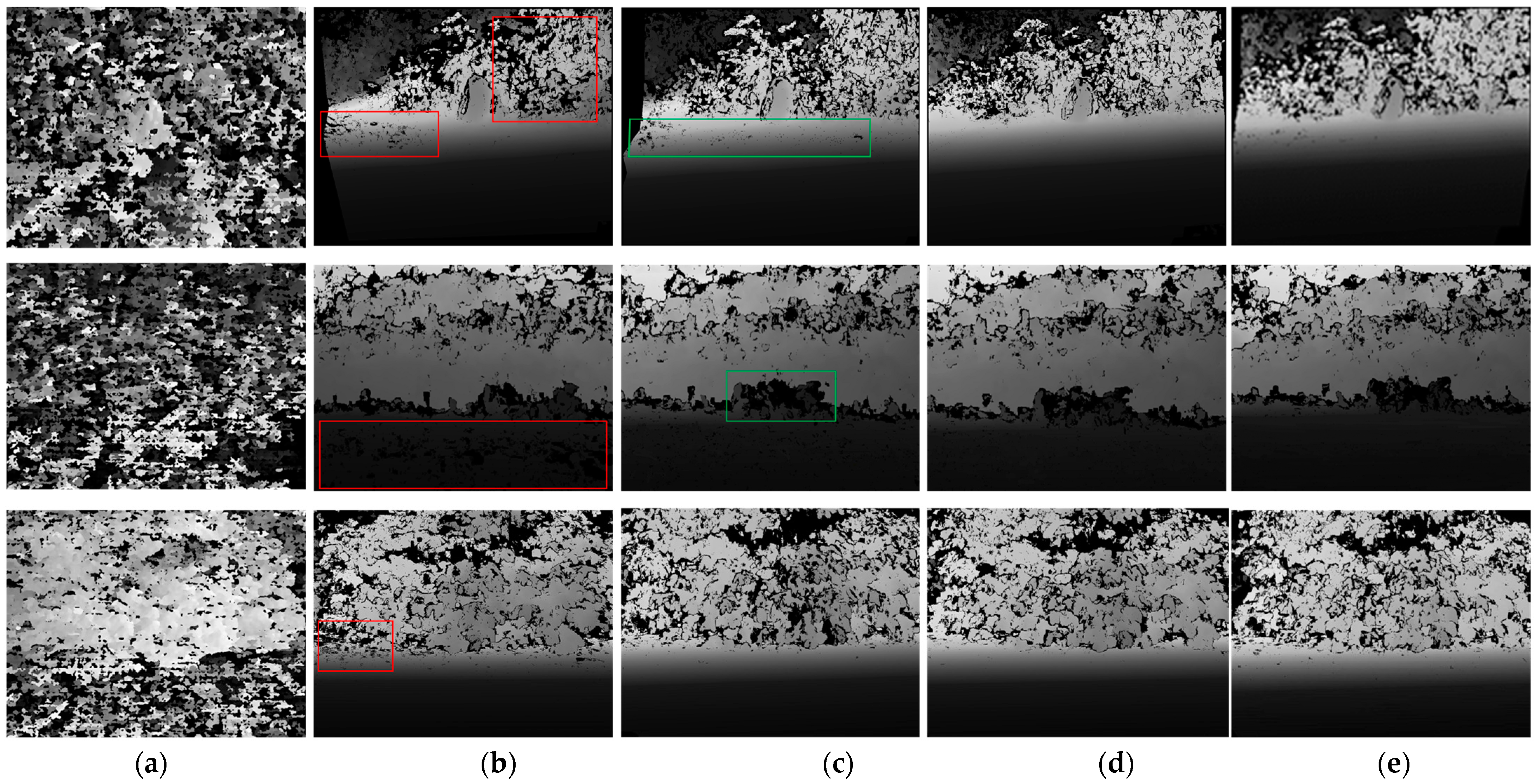
3.1. Stereo-Matching Experiments

We used the stereo camera platform to take pictures of random indoor scenes, and each image effect was arranged as an overexposure effect using light exposure. The pairs of images obtained were used to experimentally compare the currently commonly used feature detection and feature matching algorithms. The experimental results are shown in

Table 1. Performance comparison of feature detection algorithms.

Detection Algorithms	Number of Feature Points Detected by Image Pair/Points	Time Consumption for Feature Point Detection/ms
KAZE [53]	275	141
AKAZE [54]	222	120
BRISK [55]	311	276
FREAK [56]	98	56
SIFT [57]	406	952
SURF [58]	601	174
BRIEF [59]	98	92
FAST-50 [60]	514	19
FAST-40	602	27
SAD-FAST-$t$	874	32

and

Table 2. Performance comparison of several feature extraction algorithms using FLANN matching.

Algorithms	Matching Success Rate/%	Matching Time/ms
ORB [61]	64	36.6
SIFT [57]	87.7	156.7
SURF [58]	79.4	312.1
AKAZE [54]	71.6	41.7
BRISK [55]	75.2	46.3
ORB + SURF	81.4	73.2
AKAZE + SURF	82.1	149.4
SIFT + SURF	76.7	243.9
BRISK + SURF	79.6	376.1
KAZE + SURF	81.9	69.4
SAD-FAST-$t$ + SURF	85.1	57.9

.

Table 1 compares the performances of the commonly used feature detection algorithms, where FAST-50 and FAST-40 indicated that the threshold value was set to 50 and 40 when deploying the FAST detection algorithm, respectively, and SAD-FAST-$t$ indicated that the threshold value was a self-adaptive threshold $t$ when deploying the SAD-FAST detection algorithm. As can be seen from Table 1, the FAST series feature detection algorithms not only had much lower computation times than the seven other algorithms when performing feature detection for any scene but also detected more feature points than the other algorithms. Furthermore, the use of our proposed self-adaptive-threshold SAD-FAST detection algorithm showed that the improved algorithm was significantly more adaptable and could detect 70% and 45.1% more feature points than FAST-50 and FAST-40, respectively.

Figure 9 shows the experimental results for the feature matching with the FLANN matching algorithm and the Mahalanobis distance determination after feature extraction with several feature extraction algorithms. Figure 9a–e show the result plots for the ORB algorithm, SURF algorithm, SIFT algorithm, AKAZE algorithm, and BRISK algorithm after extracting the image features and then using FLANN matching, respectively. Figure 9f–j show the results of feature matching using FLANN for five types of “disorganized” stereo-matching systems; namely, ORB + SURF, AKAZE + SURF, SIFT + SURF, BRISK + SURF, and KAZE + SURF. Figure 9k shows a result graph for the use of the SAD-FAST algorithm for feature detection, the SURF feature description algorithm for the obtained feature points, and, finally, the FLANN matching algorithm for matching. Table 2 shows the matching performances of several corresponding feature extraction algorithms. From Table 2, we can see that our proposed SAD-FAST feature detection + SURF feature description + FLANN matching algorithm, in a combination of stereo-matching experiments, was slightly slower than the ORB algorithm, AKAZE algorithm, and BRISK algorithm at matching in real time when dealing with feature matching in scenes strongly affected by illumination, but the number of feature-point pairs and the matching success rate were much higher than for these three algorithms. Compared with the SURF and SIFT algorithms, the matching success rate with our proposed combination was slightly lower than that with the SIFT algorithm, but the real-time performance was much higher than with these two algorithms. Compared with the other five types of recombinant stereo-matching systems, our proposed combination is clearly in an advantageous position in terms of the number of detected feature points, matching success rate, and real-time performance.

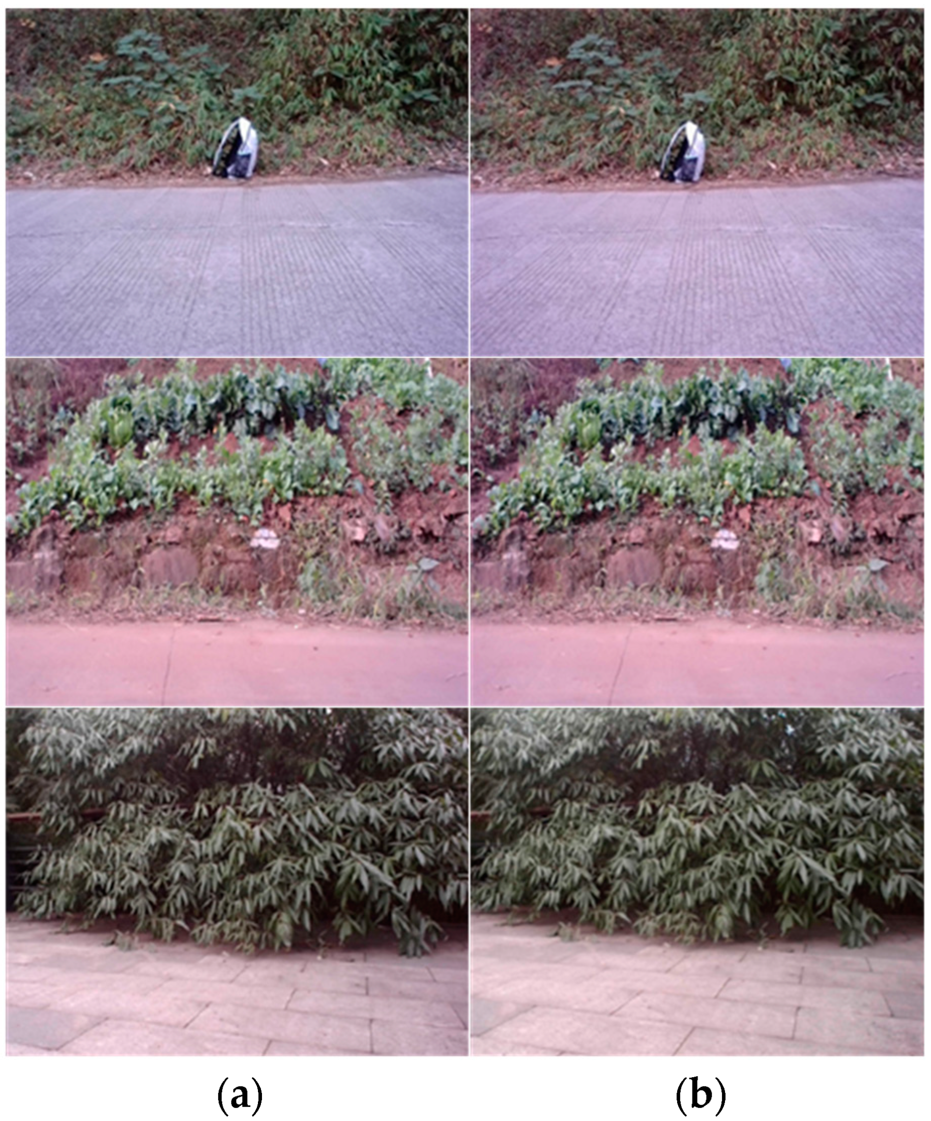
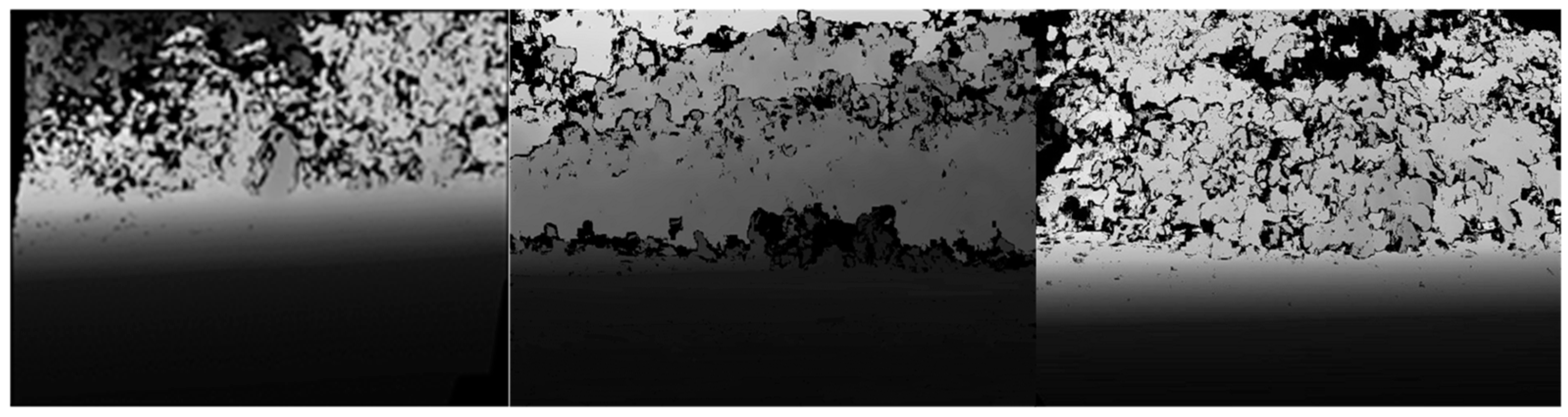
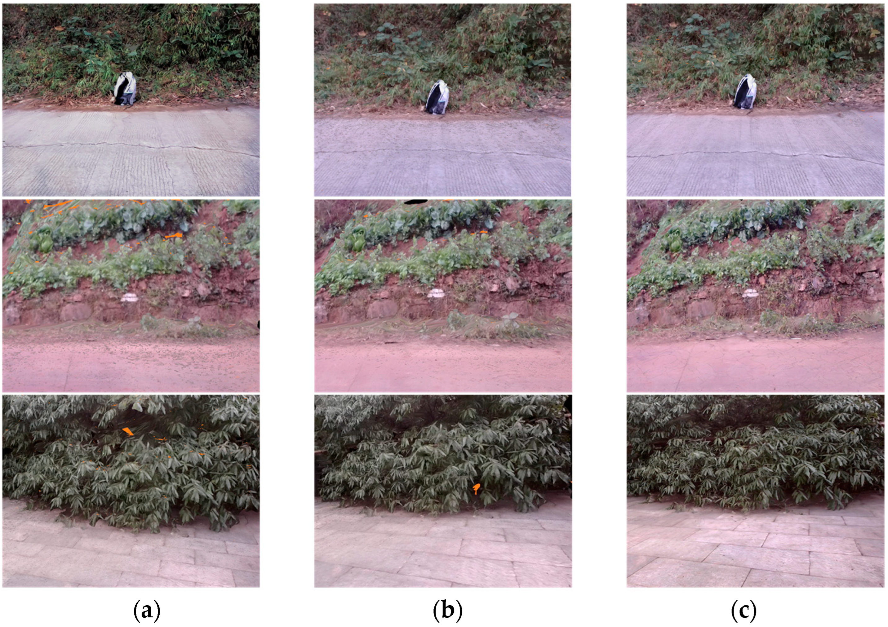
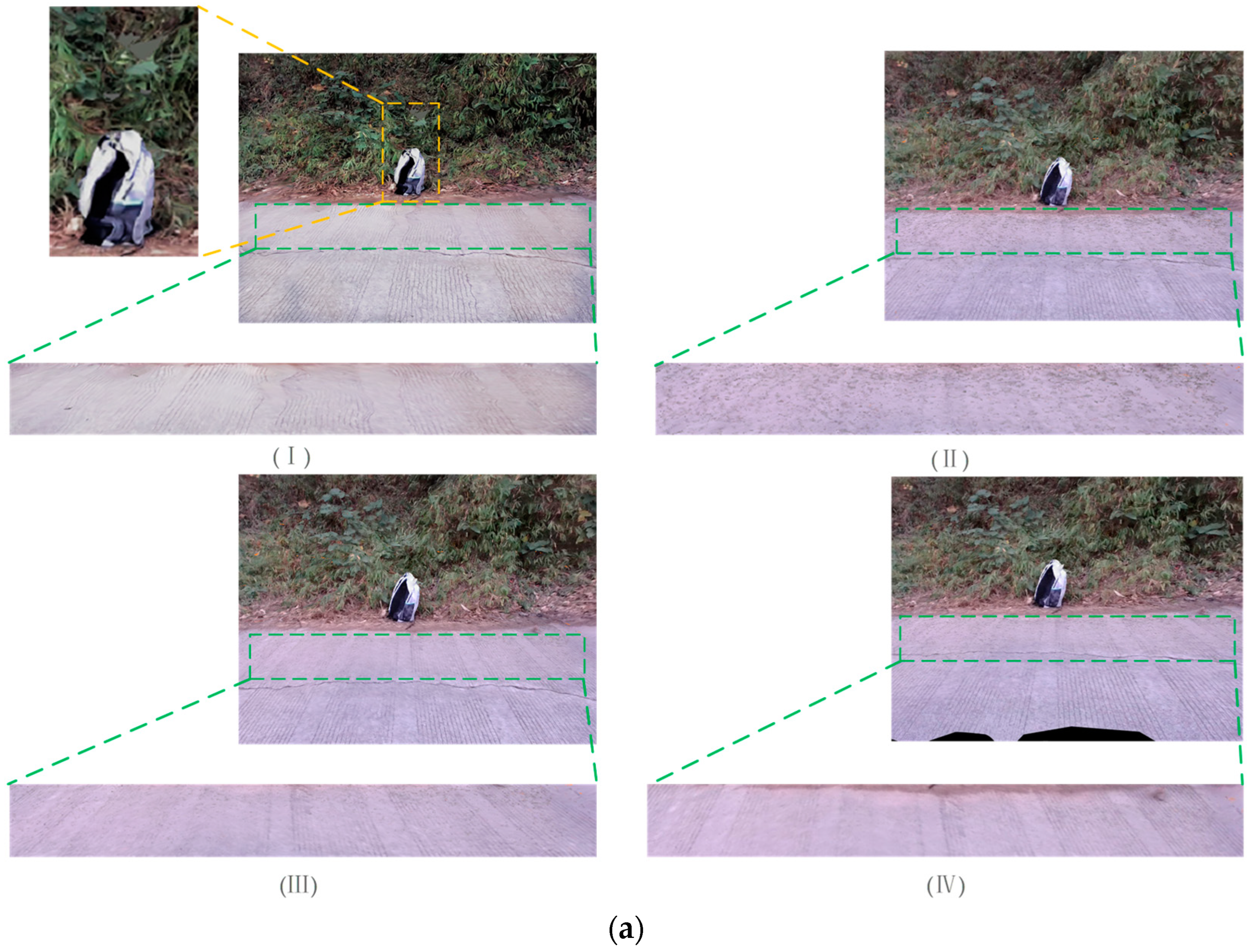
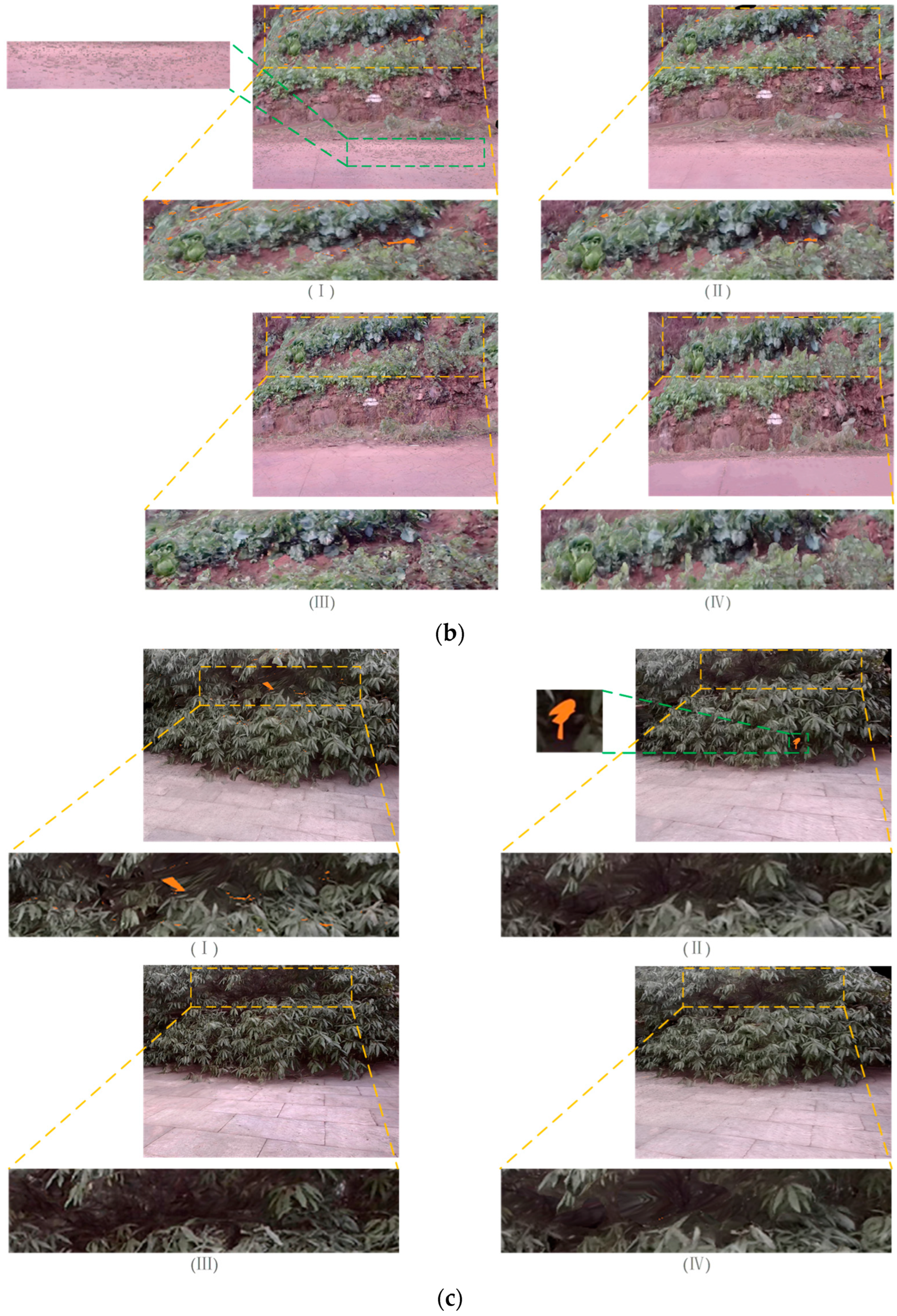
3.2. Experimental Results for Feature Extraction with Depth Value Calculation

Figure 10 shows three image pairs acquired with our stereo camera experiment platform. The acquisition areas were concrete pavements in different natural scenes.

We performed stereo matching based on the proposed SAD-FAST feature detection, SURF feature descriptor, and FLANN matching algorithms, combined with an overall strategy of discarding feature points that were too close together, followed by extracting features and calculating depth values. The disparity results are shown in Figure 11.

It can be seen that our disparity result maps connected very smoothly in the flat areas with weak textures, showing good results without any large voids.

Figure 12a shows the results of the feature extraction for the three scenes when it was difficult to extract feature points from flat areas. The distributions of the feature points in the figures were mostly concentrated in areas with large gradient changes; that is, bushes, crops, trees, and areas where the road surface and strong texture information divided in the original figures. For the road surface, very few feature points were extracted in the slightly wider area of the existing crack defect site. For most of the flat areas with weak depth variation and narrow fracture areas, it was not possible to extract feature points, resulting in serious loss of 3D information in such areas. Figure 12b shows the results of feature point extraction with our proposed GVDS feature extraction algorithm. It can be seen that not only did it satisfy the requirement for more feature points in the region with strong texture information but it also extracted feature points in the region with weak depth variation, thus avoiding the loss of 3D information in this region and achieving the overall desired 3D reconstruction effect.

Figure 13a shows the effect for the 3D point cloud scene when it was not possible to extract the feature points of the flat area, and Figure 13b shows the effect for the 3D point cloud scene after the feature points were extracted using our algorithm.

Figure 14a shows the final reconstruction effect for the unextracted flat area after texture mapping, Figure 14b shows the reconstruction effect for the extracted flat area after texture mapping, and Figure 14c shows the top view of the reconstructed flat area. It can be seen that, in Figure 14a, large areas of 3D information were lost due to the inability to extract feature points, so the reconstruction effects for such critical parts as cracks and pavements were extremely poor, which is what directly leads to the difficulty of forming a visualized 3D model with integrity and practicality. As can be seen in Figure 14b, our proposed algorithm retained the feature points with important texture information while extracting the feature points in the nearly texture-free area so that the 3D information for such areas could be obtained and the final 3D model built. At the same time, we combined the reconstruction with the top view in Figure 14c, and the reconstruction effect for the flat areas reached a fine level that can be used for engineering projects after texture mapping. In summary, it can be seen that our proposed algorithm is competent for the reconstruction task with arbitrary unstructured natural scenes and demonstrated good reconstruction results and nearly realistic texture information.

The reader can refer to Table 2 for a comprehensive comparison of traditional algorithms. We chose three types of algorithms—SURF and SIFT, which had higher matching success rates, and ORB, which had slightly lower time consumption—to perform feature detection and feature description, respectively, and then used the FLANN feature matching algorithm to perform comparison experiments based on Euclidean distance. The disparity map derived after the stereo-matching experiment was mechanically extracted from the feature points, and then the 3D coordinates were calculated to finally reconstruct the 3D point cloud for the same scenes, as shown in Figure 15.

It can be seen that, for unstructured and large scenes with significant differences in the intensity of texture information in different regions, the traditional algorithms selected too few feature points and the feature information contained was not optimal, resulting in poor point cloud effect maps that could no longer be triangulated to achieve a complete and effective structured network and, therefore, could not meet the requirements of high-precision 3D models.

We conducted 3D reconstruction real-time performance tests using the three scene images taken with the stereo-camera platform, and the average test data for the images are shown in

Table 3. Real-time testing of different traditional algorithms.

3D Reconstruction Steps	Traditional Algorithms/ms			Our Algorithm/ms
	SURF [58]	SIFT [57]	ORB [61]	SAD-FAST + SURF + GVDS
Camera and image pretreatments	47.361 + 51.12	47.361 + 51.12	47.361 + 51.12	47.361 + 51.12
Stereo-matching experiment	336.27	182.61	61.632	64.301
Depth value calculation	57.94	42.46	25.73	17.82
Triangulation and texture mapping	---	---	---	35.134

. It can be seen that our algorithm showed a large improvement in real-time performance over the traditional, widely used 3D reconstruction techniques when reconstructing such unstructured scenes with intricate texture information, and it can meet the high real-time performance standard.

Deep learning has made excellent progress in many computer-vision problems in recent years, and the field of stereo matching in 3D reconstruction is certainly no exception. We referred to the large framework for each network for stereo matching based on deep learning and found that the most frequently used stereo models usually include four steps; that is, feature extraction, cost volume construction, cost aggregation, and disparity regression. We used three network structures for stereo matching from [62,63,64] to derive the disparity maps and the GVDS algorithm to extract feature points based on the corresponding disparity maps and finally mapped the texture features of the 2D images to 3D point clouds to form the final visualized 3D models. In order to allow a good comparison of the disparity maps derived from different algorithms, we used the ApplyColorMap function, which is commonly used in the OpenCV library for color conversion of disparity maps, to convert the disparity maps from [63,64] into grayscale disparity maps. They are displayed in Figure 16.

After referring to Figure 15, in order to reflect the difference between the traditional algorithms and the other four algorithms, we also selected the SURF algorithm, which was able to form the densest point cloud among the traditional algorithms, for inclusion in the disparity comparison shown in Figure 16. As can be seen in Figure 16, the traditional algorithm SURF, due to its own limitations, had difficulty in detecting a larger number of feature points when facing such scenes with nearly countless detailed textures (numerous leaves, flowers, and plants) and large, flat, diffuse reflective areas, resulting in difficulties in forming matches between image pairs and, eventually, the formation of disparity maps of very poor quality. The 3D point clouds formed by feature extraction on the basis of these disparity maps were so sparse that effective mesh skeletons could not be constructed, which was the reason why it was difficult to form the final models of texture mapping after feature extraction. The disparity maps generated by the algorithm from [62] had high numbers of voids in the junction areas of both complex and weakly textured regions of texture information in all three scenes. Although the areas with the voids were small compared to the whole disparity maps, the overconcentrated distribution led to the loss of 3D information when feature extraction was performed, and eventually voids or black impurities that did not have texture were formed in the texture models, as shown in the red boxes in Figure 16b. The disparity maps generated by the algorithm from [63] also had a few voids in the ground of scene one, and this drawback was also reflected in the final 3D model. The disparity maps generated by the algorithm from [64] did not show voids in weakly textured regions in any of the three scenes, nor did they show large voids in adjacent regions due to overly dense distribution of strong information feature points in texturally complex regions. In our proposed stereo-matching algorithm, the upper left corner of the ground in scene one had a very small number of voids compared to the algorithm from [64], but the area and size of the voids were smaller than those with the other three algorithms. Due to the low number and small area, feature points could still be extracted around the tiny voids without losing this part of the 3D information when reconstructing using our proposed GVDS algorithm. For scene two, our proposed algorithm did not show voids in the road surface, while for the junction parts of the road surface and the field canyon, due to the fineness of the weeds themselves and obscuration, the algorithm from [63], the algorithm from [64], and our algorithm all showed voids in different locations in the same area in the green box in scene two. However, since this region was not a large area with continuous disparity loss, 3D information could still be obtained with the 3D reconstruction using GVDS. In scene three, neither the algorithms from [63,64] nor our proposed algorithm showed voids, but the algorithm from [62] showed a too obvious hole in the junction parts.

In summary, the disparity effect developed by the algorithm from [62] was significantly weaker than that of the other three algorithms when they were utilized for disparity comparison. The algorithm from [63] was weaker than the algorithm from [64] and our proposed algorithm in some regions. Our proposed algorithm showed very few voids in the upper left region of the ground in scene one and, similarly to the disparity maps formed by the algorithm from [64], it showed good disparity results in other regions of scene one and in the rest of the scenes. At the same time, it should also be noted that many of the stereo-matching algorithms proposed so far have shown excellent results compared to traditional algorithms when dealing with individual cases with almost limitless strong texture information (e.g., countless leaves along with a single leaf with a very small area compared to the overall area of the image), but it is also difficult for them to avoid a few voids, which can be studied further in the future.

We performed feature extraction using GVDS for the disparity maps formed by the three algorithms from [62,63,64] on the basis of Figure 16 and finally formed 3D models, as shown in Figure 17.

It can be seen that, in scene one in Figure 17a, because the disparity map of the algorithm from [62] had more concentrated and slightly more numerous holes in the junction area between the road surface and the bushes, distortion of the fine line pattern of the road surface and of the schoolbag ultimately resulted during texture mapping. In scene one in Figure 17a, firstly, the disparity map formed by the algorithm from [62] had a large number of large voids on the road surface, which directly led to the presence of a large number of black impurities on the road surface in the 3D model. It can also be seen that there were some yellow voids in the area with crops in the field canyons, which were caused by the absence of point clouds. In scene three in Figure 17a, the 3D model formed by the algorithm from [62] had a slight hollow in the depths of the leaves. For the 3D model formed with the algorithm from [63], there were more black impurities on the pavement in scene one due to the existence of a disparity map with a wide distribution of fine voids on the pavement. For scene two, the 3D model had very few cavities in the crop area of the field canyon. In scene three, there was a cavity in the ground and foliage junction area. In the 3D models of the three scenes formed by the algorithm from [64], only a few black impurities appeared in some areas of the road surface in scene one, and the remaining two scenes were well-reconstructed.

For comparison, we show details for the areas that were not easily observed in the three scenes reconstructed by the different algorithms in Figure 18.

As can be seen from Figure 9, since the proposed stereo-matching algorithm and system could detect a large number of feature points and the mismatching rate was very low when stereo matching was performed, the 3D reconstruction based on the good disparity maps formed could produce good 3D models, and they were not inferior to those of the deep learning stereo-matching algorithm. We performed real-time tests with different algorithms and the results are shown in

Table 4. Real-time testing of different deep learning algorithms.

3D Reconstruction Steps	Traditional Algorithms/ms			Our Algorithm/ms
	[62]	[63]	[64]
Camera and image pretreatments	47.361 + 51.12	47.361 + 51.12	47.361 + 51.12	47.361 + 51.12
Stereo-matching experiment	137	263.2	243	64.301
Triangulation and texture mapping	32.17	35.784	37.263	35.134

.

As can be seen, in the stereo-matching stage, the stereo-matching algorithms using deep learning consumed more time because they contained more network structures and modules, and our proposed stereo-matching algorithm was faster than the algorithm from [62], which is known for its speed, on the basis of the good disparity results achieved. In the 3D reconstruction task overall, our proposed algorithms showed better real-time performance and can better meet the needs of engineering applications

4. Discussion

In summary, our proposed algorithm showed good results in the corresponding steps in stereo-vision reconstruction, and none of the other algorithms achieved the desired reconstruction of unstructured, weakly textured scenes on the basis of the same level of experimental equipment. Since the experimental platform utilized only consisted of a pair of stereo cameras that could not generate pgm files to obtain disparity truth values as 3D laser instruments can, the evaluation index step of comparing disparity truth values could not be performed. In future research, it is our aim to select higher-performance stereo cameras and explore better reconstruction algorithms to achieve more complex scene reconstruction. Meanwhile, our algorithms should be able to demonstrate excellent applicability across a wide range of national road infrastructure projects (bridges, tunnels, etc.) around the world.

5. Conclusions

Aiming at the task of 3D reconstruction of unstructured scenes with differing intensity texture information, this paper proposed a 3D scene reconstruction method that can meet the requirements for high precision and good real-time performance. A new stereo-matching system was first used on the preprocessed 2D images; that is, the SAD-FAST feature detection with an improved self-adaptive threshold value was used to find the key points, and then the SURF descriptor and FLANN matcher were used with the Mahalanobis distance to reduce the mismatching to obtain the disparity maps. Next, the GVDS algorithm was used to adjust the distribution area of the feature points to retain the 3D information for the flat area with weak depth variation, which made the reconstruction effect more realistic and the reconstruction process more efficient. Experiments proved that our method had high accuracy and good real-time performance unmatched by traditional algorithms when facing a large range of unstructured scenes for reconstruction, and the proposed algorithm had strong robustness and wide applicability, making it capable of performing most 3D scene reconstruction tasks.

References

1. Chen, Y.; Wu, Z.; Wang, Z.; Song, Y.B.; Ling, Y.G.; Bao, L.C. Self-supervised learning of detailed 3D face reconstruction. IEEE Trans. Image Process. 2019, 29, 8696–8705. [Google Scholar] [CrossRef] [PubMed]
2. Zheng, T.X.; Huang, S.; Li, Y.F.; Feng, M.C. Key techniques for vision based 3D reconstruction: A review. Acta Autom. Sin. 2020, 46, 631–652. [Google Scholar]
3. Tewari, A.; Zollhöfer, M.; Bernard, F.; Garrido, P.; Kim, H.; Perez, P.; Theobalt, C. High-Fidelity Monocular Face Reconstruction Based on an Unsupervised Model-Based Face Autoencoder. IEEE Trans. Pattern Anal. Mach. Intell. 2020, 42, 357–370. [Google Scholar] [CrossRef] [PubMed]
4. Zhong, Y.; Wang, S.; Xie, S. 3D Scene Reconstruction with Sparse LiDAR Data and Monocular Image in Single Frame. SAE Int. J. Passeng. Cars-Electron. Electr. Syst. 2017, 11, 48–56. [Google Scholar] [CrossRef]
5. Chen, Y.; Li, Z.; Zeng, T. Research and Design of 3D Reconstruction System Based on Binocular Vision. Int. Core J. Eng. 2019, 5, 29–35. [Google Scholar]
6. Jian, X.; Chen, X.; He, W.; Gong, X. Outdoor 3D reconstruction method based on multi-line laser and binocular vision. IFAC-PapersOnLine 2020, 53, 9554–9559. [Google Scholar] [CrossRef]
7. Hsu, G.J.; Liu, Y.; Peng, H. RGB-D-Based Face Reconstruction and Recognition. IEEE Trans. Inf. Forensics Secur. 2014, 9, 2110–2118. [Google Scholar] [CrossRef]
8. Gao, Y.P.; Leif, K.; Hu, S.M. Real-Time High-Accuracy Three-Dimensional Reconstruction with Consumer RGB-D Cameras. ACM Trans. Graph. 2018, 37, 1–16. [Google Scholar]
9. Huan, L.; Zheng, X.; Gong, J. GeoRec: Geometry-enhanced semantic 3D reconstruction of RGB-D indoor scenes. ISPRS J. Photogramm. Remote Sens. 2022, 186, 301–314. [Google Scholar] [CrossRef]
10. Wang, D.; Deng, H.; Li, X.; Tian, X. 3D reconstruction of intelligent driving high-precision maps with location information convergence. J. Guilin Univ. Electron. Technol. 2019, 39, 182–186. [Google Scholar]
11. Cai, Y.; Lin, X. Design of 3D reconstruction system for laser Doppler image based on virtual reality technology. Laser J. 2017, 38, 122–126. [Google Scholar]
12. Lu, S.; Luo, H.; Chen, J.; Gao, M.; Liang, J. Application of 3D printing technology in the repair and reconstruction of bone defect in knee joint: One clinical case report. Chin. J. Clin. Anat. 2021, 39, 732–736. [Google Scholar]
13. Shah, F.M. Condition assessment of ship structure using robot assisted 3D-reconstruction. Ship Technol. Res. 2021, 68, 129–146. [Google Scholar] [CrossRef]
14. Fahim, G.; Min, K.; Zarif, S. Single-View 3D Reconstruction: A Survey of Deep Learning Methods. Comput. Graph. 2021, 94, 164–190. [Google Scholar] [CrossRef]
15. Gao, X.; Hen, S.; Zhu, L.; Shi, T.X.; Wang, Z.H.; Hu, Z.Y. Complete Scene Reconstruction by Merging Images and Laser Scans. IEEE Trans. Circuits Syst. Video Technol. 2020, 30, 3688–3701. [Google Scholar] [CrossRef]
16. Pepe, M.; Alfio, V.S.; Costantino, D. UAV Platforms and the SfM-MVS Approach in the 3D Surveys and Modelling: A Review in the Cultural Heritage field. Appl. Sci. 2023, 12, 886. [Google Scholar] [CrossRef]
17. Kumar, S.; Dai, Y.; Li, H. Monocular Dense 3D Reconstruction of a Complex Dynamic Scene from Two Perspective Frames. In Proceedings of the ICCV, Honolulu, HI, USA, 21–26 July 2017; pp. 4659–4667. [Google Scholar]
18. Chen, H.C. Monocular Vision-Based Obstacle Detection and Avoidance for a Multicopter. IEEE Access 2019, 7, 16786–16883. [Google Scholar] [CrossRef]
19. Wan, Y.; Shi, M.; Nong, X. UAV 3D Reconstruction System Based on ZED Camera. China New Telecommun. 2019, 21, 155–157. [Google Scholar]
20. Wu, X.; Wen, F.; Wen, P. Hole-Filling Algorithm in Multi-View Stereo Reconstruction. In Proceedings of the CVMP, London, UK, 24–25 November 2015; Volume 24, pp. 1–8. [Google Scholar]
21. Wang, Z.W.; Wang, H.; Li, J. Research On 3D Reconstruction of Face Based on Binocualr Stereo Vision. In Proceedings of the 2019 International Conference, Beijing, China, 18–20 October 2019. [Google Scholar] [CrossRef]
22. Han, R.; Yan, H.; Ma, L. Research on 3D Reconstruction methods Based on Binocular Structured Light Vision. Proc. J. Phys. Conf. Ser. 2021, 1744, 032002. [Google Scholar] [CrossRef]
23. Carolina, M.; Weibel, J.A.; Vlachos, P.P.; Garimella, S.V. Three-dimensional liquid-vapor interface reconstruction from high-speed stereo images during pool boiling. Int. J. Heat Mass Transf. 2020, 136, 265–275. [Google Scholar]
24. Zhou, J.; Han, S.; Zheng, Y.; Wu, Z.; Yang, Y. Three-Dimensional Reconstruction of Retinal Vessels Based on Binocular Vision. Chin. J. Med. 2020, 44, 13–19. [Google Scholar]
25. Cai, Y.T.; Liu, X.Q.; Xiong, Y.J.; Wu, X. Three-Dimensional Sound Field Reconstruction and Sound Power Estimation by Stereo Vision and Beamforming Technology. Appl. Sci. 2021, 11, 92. [Google Scholar] [CrossRef]
26. Zhai, G.; Zhang, W.; Hu, W.; Ji, Z. Coal Mine Rescue Robots Based on Binocular Vision: A Review of the State of the Art. IEEE Access 2020, 8, 130561–130575. [Google Scholar] [CrossRef]
27. Wang, Y.; Deng, N.; Xin, B.J.; Wang, W.Z.; Xing, W.Y.; Lu, S.G. A novel three-dimensional surface reconstruction method for the complex fabrics based on the MVS. Opt. Laser Technol. 2020, 131, 106415. [Google Scholar] [CrossRef]
28. Furukawa, Y.; Curless, B. Towards Internet-scale multi-view stereo. In Proceedings of the CVPR, San Francisco, CA, USA, 13–18 June 2010; pp. 1434–1441. [Google Scholar]
29. Mnich, C.; Al-Bayat, F. In situ weld pool measurement using stereovision. In Proceedings of the ASME, Denver, CO, USA, 19–21 July 2014; pp. 19–21. [Google Scholar]
30. Liang, Z.M.; Chang, H.X.; Wang, Q.Y.; Wang, D.L.; Zhang, Y.M. 3D Reconstruction of Weld Pool Surface in Pulsed GMAW by Passive Biprism Stereo Vision. IEEE Robot. Autom. Lett. 2019, 4, 3091–3097. [Google Scholar] [CrossRef]
31. Jiang, G. A Practical 3D Reconstruction Method for Weak Texture Scenes. Remote Sens. 2021, 13, 3103. [Google Scholar]
32. Stathopoulou, E.K.; Battisti, R.; Dan, C.; Remondino, F.; Georgopoulos, A. Semantically Derived Geometric Constraints for MVS Reconstruction of Textureless Areas. Remote Sens. 2021, 13, 1053. [Google Scholar] [CrossRef]
33. Wang, G.H.; Han, J.Q.; Zhang, X.M. A New Three-Dimensional Reconstruction Algorithm of the Lunar Surface based on Shape from Shading Method. J. Astronaut. 2009, 30, 2265–2269. [Google Scholar]
34. Woodham, R.J. Photometric Method for Determining Surface Orientation from Multiple Images. Opt. Eng. 1980, 19, 139–144. [Google Scholar] [CrossRef]
35. Horn, B.K.P.; Brooks, M.J. The Variational Approach to Shape from Shading. Comput. Vis. Graph. Image Process. 1986, 33, 174–208. [Google Scholar] [CrossRef]
36. Frankot, R.T.; Chellappa, R. A Method for Enforcing Integrability in Shape from Shading Algorithms. IEEE Trans. Pattern Anal. Mach. Intell. 1988, 10, 439–451. [Google Scholar] [CrossRef]
37. Agrawal, A.; Raskar, R.; Chellappa, R. What Is the Range of Surface Reconstructions from a Gradient Field. In Proceedings of the ECCV, Graz, Austria, 7–13 May 2006; pp. 578–591. [Google Scholar]
38. Harker, M.; O’Leary, P. Regularized Reconstruction of a Surface from its Measured Gradient Field: Algorithms for Spectral, Tikhonov, Constrained, and Weighted Regularization. J. Math. Imaging Vis. 2015, 51, 46–70. [Google Scholar] [CrossRef]
39. Queau, Y.; Durou, J.D.; Aujol, J.-F. Variational Methods for Normal Integration. J. Math. Imaging Vis. 2018, 60, 609–632. [Google Scholar] [CrossRef]
40. Queau, Y.; Durou, J.D.; Aujol, J.-F. Normal Integration: A Survey. J. Math. Imaging Vis. 2018, 60, 576–593. [Google Scholar] [CrossRef]
41. Zhang, Y.; Weiwei, X.U.; Tong, Y. Online Structure Analysis for Real-Time Indoor Scene Reconstruction. ACM Trans. Graph. 2015, 34, 1–13. [Google Scholar] [CrossRef]
42. Kim, J.; Hong, S.; Hwang, S. Automatic waterline detection and 3D reconstruction in model ship tests using stereo visive. Electron. Lett. 2019, 55, 527–529. [Google Scholar]
43. Peng, F.; Tan, Y.; Zhang, C. Exploiting Semantic and Boundary Information for Stereo Matching. J. Signal Process. Syst. 2021, 95, 379–391. [Google Scholar] [CrossRef]
44. Wang, D.; Hu, L. Improved Feature Stereo Matching Method Based on Binocular Vision. Acta Electron. Sin. 2022, 50, 157–166. [Google Scholar]
45. Haq, Q.M.; Lin, C.H.; Ruan, S.J.; Gregor, D. An edge-aware based adaptive multi-feature set extraction for stereo matching of binocular images. J. Ambient. Intell. Humaniz. Comput. 2022, 13, 1953–1967. [Google Scholar] [CrossRef]
46. Li, H.; Chen, L.; Li, F. An Efficient Dense Stereo Matching Method for Planetary Rover. IEEE Access 2019, 7, 48551–48564. [Google Scholar] [CrossRef]
47. Candès, E.; Tao, T. Signal recovery from incomplete and inaccurate measurement. Commun. Pure Appl. Math. 2005, 59, 1207–1223. [Google Scholar] [CrossRef]
48. Kong, D.W. Triangulation and Computer Three-Dimensional Reconstruction of Point Cloud Data. J. Southwest China Norm. Univ. (Nat. Sci. Ed.) 2019, 44, 87–92. [Google Scholar]
49. Dai, G. Automatic, Multiview, Coplanar Extraction for CityGML Building Model Texture Mapping. Remote Sens. 2021, 14, 50. [Google Scholar]
50. Peng, X.; Guo, X.; Centre, L. The Research on Texture Extraction and Mapping Implementation in 3D Building Reconstruction. Bull. Sci. Technol. 2014, 30, 77–81. [Google Scholar]
51. Bernardini, F.; Martin, I.M.; Rushmeier, H. High-quality texture reconstruction from multiple scans. IEEE Trans. Vis. Comput. Graph. 2001, 7, 318–322. [Google Scholar] [CrossRef]
52. Muja, M.; Lowe, D.G. Fast Approximate Nearest Neighbors with Automaticalgorithm Configuration. In Proceedings of the ICCV, Kyoto, Japan, 29 September–2 October 2009; pp. 331–340. [Google Scholar]
53. Pablo, F.A.; Adrien, B.; Andrew, J.D. KAZE Features. In Proceedings of the ECCV, Florence, Italy, 7–13 October 2012; pp. 214–227. [Google Scholar]
54. Pablo, F.A.; Nuevo, J.; Adrien, B. Fast Explicit Diffusion for Accelerated Features in Nonlinear Scale Spaces. In Proceedings of the BMVC, Bristol, UK, 9–13 September 2013. [Google Scholar] [CrossRef]
55. Leutenegger, S.; Chli, M.; Siegwart, R.Y. BRISK: Binary Robust Invariant scalable keypoints. In Proceedings of the ICCV, Barcelona, Spain, 6–13 November 2011; pp. 2548–2555. [Google Scholar]
56. Alahi, A.; Ortiz, R.; Vandergheynst, P. FREAK: Fast Retina Keypoint. In Proceedings of the CVPR, Providence, RI, USA, 16–21 June 2012; pp. 510–517. [Google Scholar]
57. Lowe, D.G. Distinctive Image Features from Scale-Invariant Keypoints. Int. J. Comput. Vis. 2004, 60, 91–110. [Google Scholar] [CrossRef]
58. Bay, H.; Tuytelaars, T.; Gool, L.V. SURF: Speeded Up Robust Features. In Proceedings of the ECCV, Graz, Austria, 7–13 May 2006; pp. 404–417. [Google Scholar]
59. Calonder, M.; Lepetit, V.; Strecha, C. BRIEF: Binary Robust Independent Elementary Feature. In Proceedings of the ECCV, Hersonissos, Greece, 5–11 September 2010; pp. 778–792. [Google Scholar]
60. Rosten, E.; Drummond, T. Machine Learning for High-Speed Corner Detection. In Proceedings of the ECCV, Graz, Austria, 7–13 May 2006; pp. 430–443. [Google Scholar]
61. Rublee, E.; Rabaud, V.; Konolige, K.; Bradski, G.R. ORB: An efficient alternative to SIFT or SURF. In Proceedings of the ICCV, Barcelona, Spain, 6–13 November 2011; pp. 2564–2571. [Google Scholar]
62. Yang, G.S.; Manela, J.; Happold, M.; Ramanan, D. Hierarchical Deep Stereo Matching on High-Resolution Images. In Proceedings of the CVPR, Long Beach, CA, USA, 16–20 June 2019. [Google Scholar] [CrossRef]
63. Xu, G.W.; Cheng, J.D.; Peng, G.; Yang, X. Attention Concatenation Volume for Accurate and Efficient Stereo Matching. In Proceedings of the CVPR, New Orleans, LA, USA, 19–24 June 2022; pp. 12981–12990. [Google Scholar]
64. Liu, B.Y.; Yu, H.M.; Long, Y.Q. Local Similarity Pattern and Cost Self-Reassembling for Deep Stereo Matching Networks. In Proceedings of the AAAI, Vancouver, BC, Canada, 22 February–1 March 2022; pp. 1647–1655. [Google Scholar]
Figure 1. Photometric 3D reconstruction models. (a) SFS; (b) PS.
Applsci 13 06407 g001
Figure 2. Steps in 3D scene reconstruction.
Applsci 13 06407 g002
Figure 3. Flow of feature matching algorithm.
Applsci 13 06407 g003
Figure 4. Schematic diagram of FAST feature detection.
Applsci 13 06407 g004
Figure 5. Flow chart for the improved SAD-FAST detection algorithm.
Applsci 13 06407 g005
Figure 6. Principle diagram for parallel optical axis depth value calculation.
Applsci 13 06407 g006
Figure 7. GVDS algorithm flow chart.
Applsci 13 06407 g007
Figure 8. Experimental platform with stereo camera.
Applsci 13 06407 g008
Figure 9. Comparison of experimental results for matching with several feature extraction algorithms using the FLANN matcher: (a) ORB [61]; (b) SIFT [57]; (c) SURF [58]; (d) AKAZE [54]; (e) BRISK [55]; (f) ORB + SURF combination; (g) AKAZE + SURF combination; (h) SIFT + SURF combination; (i) BRISK + SURF combination; (j) KAZE + SURF combination; (k) SAD-FAST + SURF combination.
Applsci 13 06407 g009aApplsci 13 06407 g009b
Figure 10. Left and right views of the scenes. (a) Left view; (b) right view.
Applsci 13 06407 g010
Figure 11. Disparity results for the three scenes.
Applsci 13 06407 g011
Figure 12. Schematic diagram of feature point extraction results: (a) non-GVDS; (b) GVDS.
Applsci 13 06407 g012
Figure 13. Point cloud maps for three scenes: (a) non-GVDS; (b) GVDS.
Applsci 13 06407 g013
Figure 14. Final reconstruction maps for the three scenes: (a) non-GVDS; (b) GVDS; (c) GVDS (top view).
Applsci 13 06407 g014
Figure 15. Point cloud maps produced by the conventional algorithms for three scenes: (a) SURF [58]; (b) SIFT [57]; (c) ORB [61].
Applsci 13 06407 g015
Figure 16. Disparity map results based on different algorithms: (a) SURF [58]; (b) [62]; (c) [63]; (d) [64]; (e) ours.
Applsci 13 06407 g016
Figure 17. Three-dimensional models: (a) [62] (b) [63]; (c) [64].
Applsci 13 06407 g017
Figure 18. Comparison of some details from the 3D models. (a) Scene one: (I) [62]; (II) [63]; (III) [64]; (IV) ours; (b) scene two: (I) [62]; (II) [63]; (III) [64]; (IV) ours; (c) scene three: (I) [62]; (II) [63]; (III) [64]; (IV) ours.
Applsci 13 06407 g018aApplsci 13 06407 g018b