Manifolds-Based Low-Rank Dictionary Pair Learning for Efficient Set-Based Video Recognition

Abstract

As an important research direction in image and video processing, set-based video recognition requires speed and accuracy. However, the existing static modeling methods focus on computational speed but ignore accuracy, whereas the dynamic modeling methods are higher-accuracy but ignore the computational speed. Combining these two types of methods to obtain fast and accurate recognition results remains a challenging problem. Motivated by this, in this study, a novel Manifolds-based Low-Rank Dictionary Pair Learning (MbLRDPL) method was developed for a set-based video recognition/image set classification task. Specifically, each video or image set was first modeled as a covariance matrix or linear subspace, which can be seen as a point on a Riemannian manifold. Second, the proposed MbLRDPL learned discriminative class-specific synthesis and analysis dictionaries by clearly imposing the nuclear norm on the synthesis dictionaries. The experimental results show that our method achieved the best classification accuracy (100%, 72.16%, 95%) on three datasets with the fastest computing time, reducing the errors of state-of-the-art methods (JMLC, DML, CEBSR) by 0.96–75.69%.

1. Introduction

With the development of imaging technology, people can increasingly easily obtain multimedia data, such as images and videos. Additionally, much multimedia data are usually stored in the form of image sets, such as personal photo albums, multi-view photo albums, and video frame sets. Therefore, studies of set-based video recognition or image set classification methods are needed.

In set-based video recognition or image set classification tasks, only the spatial information of the video is considered. Thus, the key problems of image set classification (ISC) task are how to model the image sets and how to measure the distance between model representations; additionally, the choice of modeling strategy is the basis of distance measurement. The existing ISC modeling methods can be grouped into two types: static and dynamic modeling methods. Classical static modeling methods include Covariance Discriminative Learning (CDL) [1], Multi-Model Fusion Metric Learning (MMFML) [2], etc. This type of method provides a unique modeling representation for each image set and then performs distance metric learning based on the representation. However, although the calculations of such methods are fast, their classification accuracy is usually uncompetitive.

Classical dynamic modeling methods include Image-Set-based Collaborative Representation and Classification (ISCRC) [3], Regularized Nearest Points (RNP) [4], etc. With this type of method, sparse representation or collaborative representation is usually used to simultaneously learn the representation coefficients (which is also known as dynamic modeling) and the distance between different image sets. The classification performance of dynamic modeling methods is usually more accurate than that of the static modeling methods; however, better performance is achieved at the expense of computational efficiency. For example, suppose that we have N gallery image sets. When classifying one probe image set, the dynamic modeling methods need to solve N sparse or collaborative optimization problems, which is time-consuming. To reduce the computing time required for solving N sparse or collaborative optimization problems, Liu et al. proposed the Convolutional Encoder-based Block Sparse Representation (CEBSR) [5] model to learn K discriminative dictionaries for K categories. When classifying one probe set, CEBSR only needs to solve K sparse optimization problems, and $K<N$ is satisfied. Moreover, CEBSR uses the image set matrix as the feature representation of the probe set, neglecting the importance of set modeling. Additionally, solving the sparse representation problem is time-consuming. Recently, Gu et al. proposed the projective Dictionary Pair Learning (DPL) [6] algorithm, which decomposes the original sparse representation into a linear reconstruction problem by introducing the analysis dictionaries, thereby considerably speeding up the sparse representation computing. Therefore, introducing DPL into the ISC field is a compelling idea.

To increase the efficiency and accuracy of image set classification, in this study, we developed a new Manifolds-based Low-Rank Dictionary Pair Learning (MbLRDPL) method, which combines the advantages of both static and dynamic modeling methods. Specifically, static modeling (i.e., covariance matrix or linear subspace) is first used to model each image set; second, the Manifolds-based Discriminative Dictionary Learning algorithm, i.e., MbLRDPL, is developed by introducing DPL into the ISC task. In addition, the nuclear norm is imposed on the synthesis dictionaries for further strengthening the discriminative ability. The flowchart of the proposed method is shown in Figure 1.

The rest of this paper is organized as follows: Section 2 provides an overview of related studies. In Section 3, the MbLRDPL algorithm is proposed. The experiments and results are described in Section 4. A discussion and the conclusions are outlined in Section 5 and Section 6, respectively.

2. Related Works

In this section, we review two related aspects: image set classification and dictionary learning.

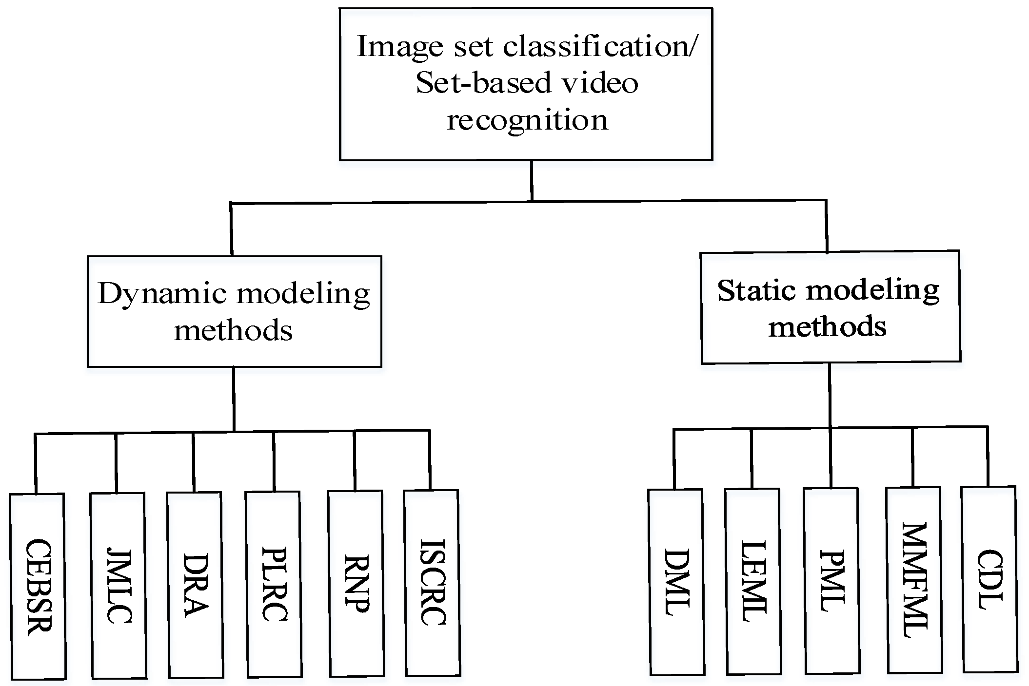
2.1. Image Set Classification

So far, many research works have been made in computer vision [7,8,9,10,11], especially in the image set classification [1,2,3,4,12,13,14,15,16,17,18] field. In this subsection, as shown in Figure 2, we briefly review two types of image set classification methods: static and dynamic modeling methods.

2.1.1. Static Modeling Methods

With static modeling methods, each image set is modeled with some unique, fixed methods, such as parametric distribution function, subspace, covariance matrix, multiorder statistics, and domain (or hypersphere). For instance, CDL [1] and Log-Euclidean Metric Learning (LEML) [13] algorithms use covariance matrices to represent image sets and then use logarithm kernels to map the modeling representations to the Hilbert space to easily measure the similarity between image sets. Projection Metric Learning (PML) [12] models each image set as a subspace (i.e., a point on a Grassmann manifold), and directly learns a projection matrix on a Grassmann manifold to reduce the computational cost. The MMFML [2] algorithm jointly uses multiple representation models to represent one image set, which aims to fully use the complementarity between different representation models. Discrete Metric Learning (DML) [14] also combines static and dynamic modeling methods; however, it ignores the importance of dictionary learning. Since static modeling can markedly reduce the sample, the computing time of static modeling methods is usually fast. However, most of these static modeling methods only focus on learning more discriminative feature representations after obtaining static models, ignoring the design of a powerful classifier, resulting in limited classification results.

2.1.2. Dynamic Modeling Methods

With dynamic modeling methods, each image set is modeled with some dynamic method, such as affine hull, convex hull, and so on. These modeling methods usually rely on learning of sparse or collaborative representation coefficients. For instance, in the ISCRC [3] algorithm, each probe image set or video was modeled as affine or convex hulls; then, these models were collaboratively reconstructed using all gallery image sets or videos. In the RNP [4] algorithm, the image sets were also modeled as affine hulls. Based on this modeling, the authors developed a new objective function to simultaneously learn the modeling coefficients and the distance metric. Similar to RNP, Dual Linear Regression Classification (DLRC) [16] also modeled image sets as affine hulls and reconstructed a virtual image using two different image sets; the distance between the two reconstruction images was used as the distance between the image sets. However, in DLRC, in each distance calculation, only two image sets were used: it cannot use the useful information from other gallery image sets. Based on DLRC, two new algorithms, Pairwise Linear Regression Classification (PLRC) [17] and Discriminative Residual Analysis (DRA) [18], were then developed by introducing different unrelated subspaces. Specifically, PLRC maximized the unrelated distance between two image sets and minimized the related distance to improve the classification results. DRA learned a projection matrix to project the reconstruction residual to a more discriminative space. In other words, the PLRC algorithm was first used to compute the related and unrelated distances between any two gallery image sets, and then, the projection matrix was used to learn a more discriminative space. Since the above related and unrelated distances were independently computed, Joint Metric Learning-based Class-specific representation (JMLC) [15] jointly learned the related and unrelated metrics and extended PLRC and DRA to the large-size image set classification task. Although dynamic modeling methods provide higher-accuracy recognition performance, they usually need to solve some sparse or collaborative optimization problems, and these problems are usually time-consuming.

2.2. Dictionary Learning

Dictionary learning has been widely studies and applied for many artificial intelligence tasks, such as image classification, image compression, image denoising, etc. To date, many dictionary learning methods have been developed, which can be categorized into unsupervised and discriminative dictionary learning methods.

2.2.1. Unsupervised Dictionary Learning Methods

Unsupervised dictionary learning methods do not use any label information in the learning process. The most well-known unsupervised dictionary learning method is K-singular value decomposition (K-SVD) [19], which combines the K-means clustering algorithm and sparse representation to learn the most accurate representation. However, because label information is not used, the discriminative abilities of these methods are limited.

2.2.2. Discriminative Dictionary Learning Methods

The discriminative dictionary learning methods consider the data’s label information to enhance the discriminative and classification abilities of the representations. Since the learned dictionaries have a stronger discriminative ability, the discriminative dictionary learning classifiers have a stronger classification ability than sparse representation classifiers. The representative discriminative dictionary learning methods include the Discriminative KSVD (D-KSVD) [20] algorithm, analysis discriminative dictionary learning (ADDL) [21], Deep Dictionary Learning (DDL) [22], Self-expressive Latent Dictionary Pair Learning (SLatDPL) [23], and CEBSR [5] algorithms, among others. However, most of them are single-image-based methods, so they cannot be effectively used in image set classification or video recognition tasks. The CEBSR algorithm was used for image set classification, but it is essentially still a single-image-based method because it used a probe image matrix to model the image set. This leads to long computing time, and the classification performance cannot be guaranteed. In addition, most of these methods need to solve some time-consuming $l_1$ optimization problems, resulting in high time complexity.

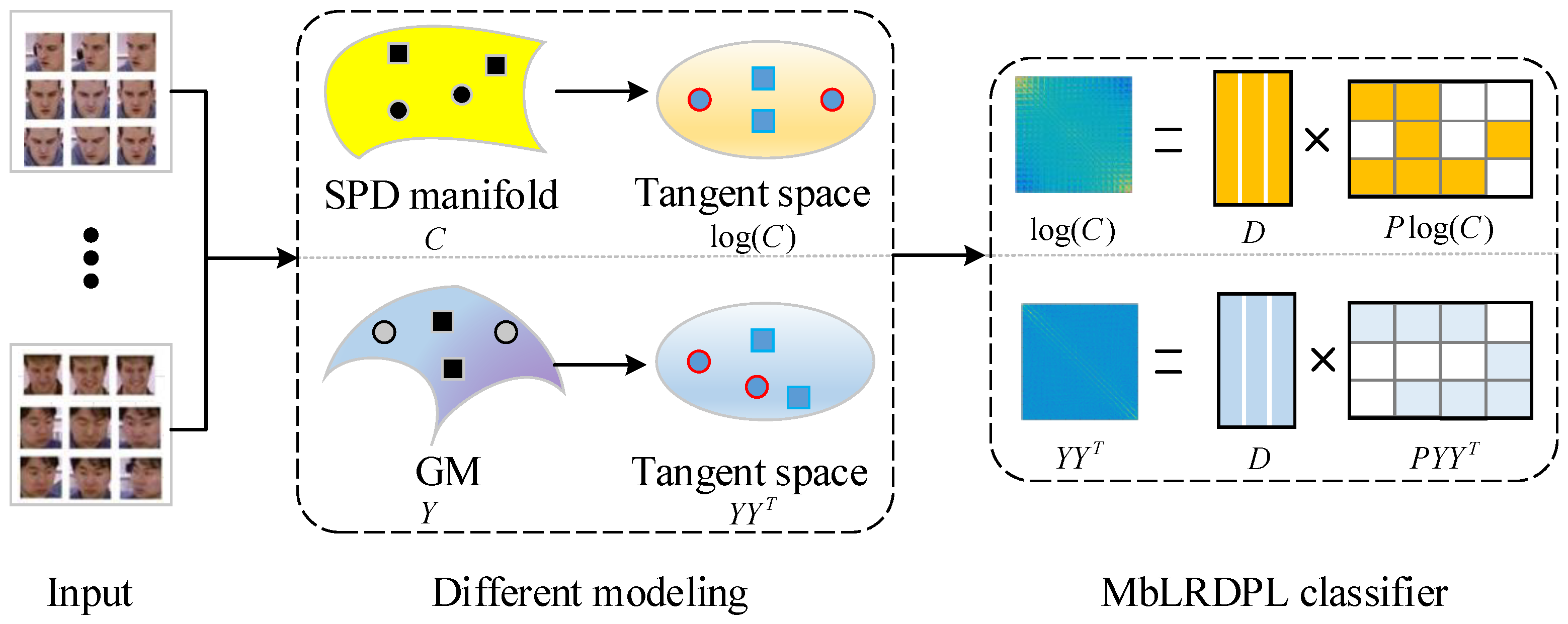
3. Manifolds-Based Low-Rank Dictionary Pair Learning

Considering the fast computing of static modeling methods and the higher recognition rate of dynamic modeling methods, in this study, we combined to achieve efficient and accurate image set classification.

3.1. Problem Formulation

Assume that we have N training image sets (gallery videos), ${\left\{X_i^k\right\}}_{i=1}^N$, which belong to K classes, where $X_i^k=[x_{i,1}^k,x_{i,2}^k,\cdots ,x_{i,m_i}^k]\in {\mathcal{R}}^{p\times m_i}$ denotes the $ith$ gallery image set which belongs to kth class. Here, $x_{i,j}^k\in {\mathcal{R}}^{p\times 1}$ denotes the jth image coming from ith gallery video, $m_i$ is the number of sample images in $X_i^k$, and p denotes the dimensions of the image sample. We also assume that in the $kth$ class, there are $n_k$ image sets. The important notations in this paper are summarized in

Table 1. Important notations used in the paper.

Notations	Description
$X,Y,C,\cdots$	a matrix
$x,d,\cdots$	a vector
$k,p,m,\cdots$	scalar
$X_i^k$	the $ith$ gallery image set from $kth$ class
$x_{i,j}^k$	the $jth$ image coming from $ith$ gallery video
⊖	the manifold replacements for subtraction
⊗	the manifold replacements for multiplication
$\left|\right|·{\left|\right|}_s^2$	the geodesic distance metric
$\left|\right|·{\left|\right|}_F$	the Frobenius norm
$\left|\right|·{\left|\right|}_1$	${\left|\right|X\left|\right|}_1={\sum }_{ij}\left|x_{ij}\right|$
$\left|\right|·{\left|\right|}_2$	the $L_2$ norm
$\left|\right|·{\left|\right|}_{*}$	the nuclear norm

.

To benefit from the advantages of static modeling method, we first use the following covariance matrix (point on a Symmetric Positive Definite (SPD) manifold) and linear subspace (point on a Grassmann Manifold (GM)) to model image sets, and we developed two submethods: MbLRDPL-SPD and MbLRDPL-GM.

3.2. MbLRDPL-SPD

MbLRDPL-SPD uses the following covariance matrix to model the image set $X_i^k$:

$$\begin{array}{c}{C}_i^k=\frac{1}{m_i-1}{\displaystyle \sum _{j=1}^{m_i}}(x_{i,j}^k-m_i){(x_{i,j}^k-m_i)}^T,\end{array}$$

(1)

where $m_i$ denotes the mean vector of image set $X_i^k$. Thus, all our gallery image sets are modeled to ${\left\{C_i^k\right\}}_{i=1}^N$, and these models are points on a Riemannian manifold; more specifically, they are points on a symmetric positive definite manifold. Thereby, we construct the following SPD-manifold-based distance learning problem:

$$\begin{array}{cc}min& \left|\right|C_i^k\ominus D_k\otimes A_i^k{\left|\right|}_s^2+{\lambda }_1\left|\right|A_i^k{\left|\right|}_1\hfill \end{array}$$

(2)

where $D_k$ and $A_i^k$ denote the $kth$ dictionary and the coding matrix on the SPD manifold, respectively; $\left|\right|C_i^k\ominus D_k\otimes A_i^k{\left|\right|}_s^2$ denotes the distance between image set $C_i^k$ and the $kth$ class image set. Here, operators ⊖ and ⊗ are the manifold replacements for subtraction and multiplication in Euclidean space, respectively. Furthermore, different from the $L_2$ norm in Euclidean space, $\left|\right|·{\left|\right|}_s^2$ is the geodesic distance metric on SPD manifolds.

The optimization problem (2) is difficult to solve because we have not explicitly defined the operators ⊖ and ⊗. However, Wang et al. [1] showed that we can embed the SPD manifold into Euclidean tangent space via the logarithm function $\log (·)$. As a result, the optimization problem (2) can be rewritten as

$$\begin{array}{cc}min& \left|\right|\log \left(C_i^k\right)-D_k{A}_i^k{\left|\right|}_F^2+{\lambda }_1\left|\right|A_i^k{\left|\right|}_1\hfill \end{array}$$

(3)

where $D_k$ and $A_i^k$ denote the dictionary and coding matrix in Euclidean spaces, respectively. However, for Equation (3), we need to solve the $L_1$-norm optimization problem, which is often computationally demanding.

To avoid the $L_1$-norm optimization problem, problem (3) is extended to the following problem by introducing the DPL algorithm:

$$\begin{array}{cc}min& {\displaystyle \sum _{k=1}^K}{\displaystyle \sum _{i=1}^{n_k}}\left|\right|\log \left(C_i^k\right)-D_k{P}_k\log \left(C_i^k\right){\left|\right|}_F^2\hfill \\ & +{\lambda }_1{\displaystyle \sum _{k=1}^K}{\displaystyle \sum _{j=1}^{{\overline{n}}_k}}\left|\right|P_k\log \left({\overline{C}}_j^k\right){\left|\right|}_F^2+{\lambda }_2{\displaystyle \sum _{k=1}^K}\left|\right|D_k{\left|\right|}_{*}\hfill \\ \mathrm{s}.\mathrm{t}.& \left|\right|d_j^k{\left|\right|}_2^2\le 1,k=1,\cdots ,K;j=1,\cdots ,m,\hfill \end{array}$$

(4)

where $D_k=[d_1^k,d_2^k,\cdots ,d_m^k]\in {\mathcal{R}}^{p\times m}$ is the synthesis dictionary; $P_k\in {\mathcal{R}}^{m\times p}$ is the analysis dictionary; m is the number of atoms in the dictionary; ${\left\{{\overline{C}}_j^k\right\}}_{j=1}^{{\overline{n}}_k}$ are the complementary data of $C_j^k$ in the whole gallery sets, i.e., all the gallery sets that do not belong to the $kth$ class; ${\overline{n}}_k$ is the number of complementary sets. Note that the first term in Equation (4) is the fidelity term, which is used to ensure that the learned dictionaries effectively reconstruct the input data. The second term is the discriminative term, which ensures that the analysis subdictionary $P_k$ can project the gallery sets of other classes into a null subspace. The third term is the nuclear norm regularization term, which is used to guarantee that the representation coefficients of samples from the same class have higher similarity.

This problem is solved in Section 3.4 to obtain the optimal dictionaries $D_k$, $P_k$, and $k=1,\cdots ,K$. When a new probe image set Z is considered, we only need to solve the following problem to obtain its label:

$$\begin{array}{c}label\left(Z\right)=\underset{k}{\arg \min }\left|\right|\log \left(C_z\right)-D_k{P}_k\log \left(C_z\right){\left|\right|}_F^2\end{array}$$

(5)

where $C_z$ is the covariance model of Z.

3.3. MbLRDPL-GM

Different from MbLRDPL-SPD, MbLRDPL-GM uses linear subspace $Y_i^k$ to model image set $X_i^k$, and the subspace matrix $Y_i^k$ can be solved by solving the following problem:

$$\begin{array}{c}{X}_i^k{X_i^k}^T=Y_i^k{\mathsf{\Delta }}_i^k{Y_i^k}^T,\end{array}$$

(6)

where ${\mathsf{\Delta }}_i^k$ is the eigenvalue matrix, and $Y_i^k$ is the eigenvectors matrix. Since the linear subspace $Y_i^k$ is located on a Grassmann manifold, we first embed it to its tangent space with $Y_i^k{\left(Y_i^k\right)}^T$.

Then, the objective function of MbLRDPL-GM can be constructed as

$$\begin{array}{cc}min& {\displaystyle \sum _{k=1}^K}{\displaystyle \sum _{i=1}^{n_k}}\left|\right|Y_i^k{Y_i^k}^T-D_k{P}_k{Y}_i^k{\left(Y_i^k\right)}^T{\left|\right|}_F^2\hfill \\ & +{\lambda }_1{\displaystyle \sum _{k=1}^K}{\displaystyle \sum _{j=1}^{{\overline{n}}_k}}\left|\right|P_k{\overline{Y}}_i^k{\left({\overline{Y}}_i^k\right)}^T{\left|\right|}_F^2+{\lambda }_2{\displaystyle \sum _{k=1}^K}\left|\right|D_k{\left|\right|}_{*}\hfill \\ \mathrm{s}.\mathrm{t}.& \left|\right|d_j^k{\left|\right|}_2^2\le 1,k=1,\cdots ,K;j=1,\cdots ,m,\hfill \end{array}$$

(7)

where ${\overline{Y}}_i^k$ is the complementary matrix.

This problem is solved in Section 3.4 to obtain the optimal dictionaries $D_k$, $P_k$, and $k=1,\cdots ,K$. When a new probe image set Z is considered, we only need to solve the following problem to obtain its label:

$$\begin{array}{c}label\left(Z\right)=\underset{k}{\arg \min }\left|\right|Y_z{Y}_z^T-D_k{P}_k{Y}_z{Y}_z^T{\left|\right|}_F^2\end{array}$$

(8)

where $Y_z$ is the subspace model of Z.

3.4. Optimization

Here, we use symbol M to represent the modeling of the image sets, i.e., M can be a linear subspace Y or a covariance matrix C. Additionally, we use the symbol E to represent the Euclidean tangent space representation of M (i.e., E can be $\log \left(M\right)$ or $M{M}^T$). Thus, the optimization problems (4) and (7) can be rewritten as

$$\begin{array}{cc}min& {\displaystyle \sum _{k=1}^K}{\displaystyle \sum _{i=1}^{n_k}}\left|\right|E_i^k-D_k{P}_k{E}_i^k{\left|\right|}_F^2+{\lambda }_1{\displaystyle \sum _{k=1}^K}{\displaystyle \sum _{j=1}^{{\overline{n}}_k}}\left|\right|P_k{\overline{E}}_i^k{\left|\right|}_F^2+{\lambda }_2{\displaystyle \sum _{k=1}^K}\left|\right|D_k{\left|\right|}_{*}\hfill \\ \mathrm{s}.\mathrm{t}.& \left|\right|d_j^k{\left|\right|}_2^2\le 1,k=1,\cdots ,K;j=1,\cdots ,m,\hfill \end{array}$$

(9)

Since our objective function (9) is a nonconvex problem, it cannot be directly solved. Hence, the Alternating Direction Method of Multipliers (ADMM) method is used to iteratively optimize it. Specifically, to facilitate the solving of the objective function, some auxiliary variables $A_i^k$ and $J_k$, $k=1,\cdots ,K$, $i=1,\cdots ,n_k$ are introduced. Thus, problem (9) becomes

$$\begin{array}{cc}min& {\displaystyle \sum _{k=1}^K}{\displaystyle \sum _{i=1}^{n_k}}\left|\right|E_i^k-D_k{A}_i^k{\left|\right|}_F^2+{\lambda }_1{\displaystyle \sum _{k=1}^K}{\displaystyle \sum _{j=1}^{{\overline{n}}_k}}\left|\right|P_k{\overline{E}}_j^k{\left|\right|}_F^2\hfill \\ & +{\lambda }_2{\displaystyle \sum _{k=1}^K}\left|\right|J_k{\left|\right|}_{*}+\tau {\displaystyle \sum _{k=1}^K}{\displaystyle \sum _{i=1}^{n_k}}\left|\right|P_k{E}_i^k-A_i^k{\left|\right|}_F^2\hfill \\ & +\frac{\mu }{2}{\displaystyle \sum _{k=1}^K}\left|\right|J_k-(D_k+\frac{Z}{\mu }){\left|\right|}_F^2\hfill \\ \mathrm{s}.\mathrm{t}.& \left|\right|d_j^k{\left|\right|}_2^2\le 1,k=1,\cdots ,K;j=1,\cdots ,m,\hfill \end{array}$$

(10)

where $\tau$ and $\mu$ are penalty parameters, and Z is the Lagrange multiplier. The above problem can be solved with the alternating minimization method, i.e., fix other variables and update the remaining variables in turn.

(1) Fix the other variables and update $A_i^k$. $A_i^k$ can be obtained by solving the following optimization problem:

$$\begin{array}{cc}{A_i^k}^{*}& \hfill =\underset{A_i^k}{\arg \min }\left|\right|E_i^k-D_k{A}_i^k{\left|\right|}_F^2+\tau \left|\right|P_k{E}_i^k-A_i^k{\left|\right|}_F^2\end{array}$$

(11)

After solving Equation (11), we can obtain the following closed-form solution:

$$\begin{array}{c}{A}_i^k={(D_k^T{D}_k+\tau I)}^{-1}(D_k^T{E}_i^k+\tau P_k{E}_i^k)\end{array}$$

(12)

(2) Fix the other variables and update $P_k$ by solving the problem:

$$\begin{array}{cc}{P_k}^{*}& =\underset{P_k}{\arg \min }{\lambda }_1{\displaystyle \sum _{j=1}^{{\overline{n}}_k}}\left|\right|P_k{\overline{E}}_j^k{\left|\right|}_F^2+\tau {\displaystyle \sum _{i=1}^{n_k}}\left|\right|P_k{E}_i^k-A_i^k{\left|\right|}_F^2\hfill \end{array}$$

(13)

After solving Equation (13), we can obtain the following closed-form solution:

$$\begin{array}{cc}{P}_k& \hfill =\tau {\displaystyle \sum _{i=1}^{n_k}}{A}_i^k{\left(E_i^k\right)}^T{({\lambda }_1{\displaystyle \sum _{j=1}^{{\overline{n}}_k}}{\overline{E}}_j^k{({\overline{E}}_j^k)}^T+\tau {\displaystyle \sum _{i=1}^{n_k}}{E}_i^k{\left(E_i^k\right)}^T+\gamma I)}^{-1}\end{array}$$

(14)

where $\gamma ={10}^{-4}$.

(3) Fix the other variables and update $D_k$ by solving the problem:

$$\begin{array}{c}{D_k}^{*}=\underset{D_k}{\arg \min }{\displaystyle \sum _{i=1}^{n_k}}\left|\right|E_i^k-D_k{A}_i^k{\left|\right|}_F^2\hfill \\ +\frac{\mu }{2}\left|\right|J_k-(D_k+\frac{Z}{\mu }){\left|\right|}_F^2+\rho \left|\right|D_k-S_k+T_k{\left|\right|}_F^2\hfill \end{array}$$

(15)

where $S_k$ is the auxiliary variables, $T_k$ is the Lagrange multiplier, and $\rho$ is the penalty parameter. This problem can be solved by iteratively computing the following equations:

$$\left\{\begin{array}{c}{D}_k=(2{\displaystyle \sum _{i=1}^{n_k}}{E}_i^k{A_i^k}^T+2\rho (S_k-T_k)+\mu J_k-Z){(2{\displaystyle \sum _{i=1}^{n_k}}{A}_i^k{A_i^k}^T+2\rho I+\mu I)}^{-1},\hfill \\ s_j^k=\left\{\begin{array}{cc}{d}_j^k+t_j^k,\hfill & \mathrm{if}\sqrt{\left|\right|\rho d_j^k+\rho t_j^k{\left|\right|}_2^2}=\rho \hfill \\ \frac{\rho d_j^k+\rho t_j^k}{\sqrt{\left|\right|\rho d_j^k+\rho t_j^k{\left|\right|}_2^2}},\hfill & \mathrm{if}\sqrt{\left|\right|\rho d_j^k+\rho t_j^k{\left|\right|}_2^2}>\rho \hfill \end{array}\right.\hfill \\ T_k=T_k+(D_k-S_k),\hfill \end{array}\right.$$

(16)

where $S_k=[s_1^k,s_2^k,\cdots ,s_m^k]$ and $T_k=[t_1^k,t_2^k,\cdots ,t_m^k]$.

(4) Fix the other variables and update $J_k$ by solving the problem:

$$\begin{array}{c}{J_k}^{*}=\underset{J_k}{\arg \min }{\lambda }_2\left|\right|J_k{\left|\right|}_{*}+\frac{\mu }{2}\left|\right|J_k-(D_k+\frac{Z}{\mu }){\left|\right|}_F^2\hfill \end{array}$$

(17)

This problem can be directly solved by the singular value thresholding (SVT) [24] operator ${\mathbb{D}}_{·}(·)$

$$\begin{array}{c}{J}_k={\mathbb{D}}_{{\lambda }_2/\mu }(D_k+\frac{Z}{\mu })\hfill \end{array}$$

(18)

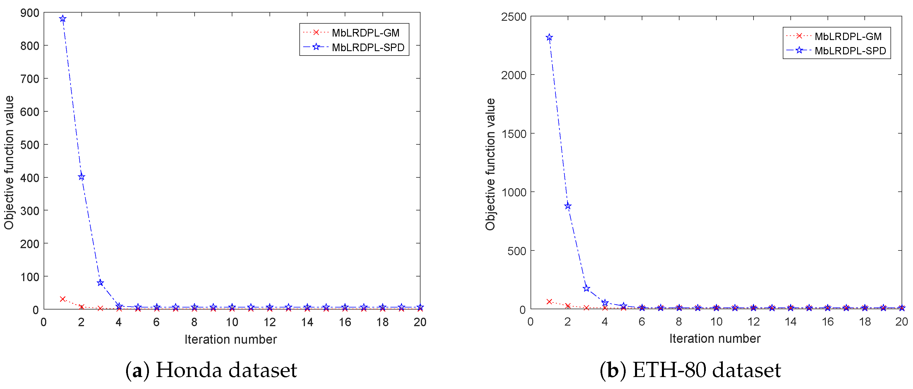
4. Experimental Results and Analysis

To test the validity of the MbLRDPL method, extensive comparison experiments were performed on two challenging visual tasks, i.e., set-based video face recognition and set-based object classification. The comparison methods include static modeling methods: CDL, PML, LEML, MMFML and DML; dynamic modeling methods: ISCRC, RNP, DLRC, PLRC, DRA and JMLC; dictionary learning methods: D-KSVD, ADDL, DDL, SLatDPL, CEBSR. Among them, DML, JMLC, and CEBSR are the state-of-the-art methods. Moreover, to further reduce the computing time, we first transformed the modeling matrix $\log \left(C_i^k\right)$ or $Y_i^k{\left(Y_i^k\right)}^T$ into a vector and then performed Principal Component Analysis (PCA) [25] to reduce its dimensions. Our experimental environment was as follows: MATLAB (R2016b), Intel(R) Core(TM) i5 (3.0 GHz) with 24 GB of RAM. The codes of this method will be available on 10 January 2023 via https://github.com/xzgao/MbLRDPL.

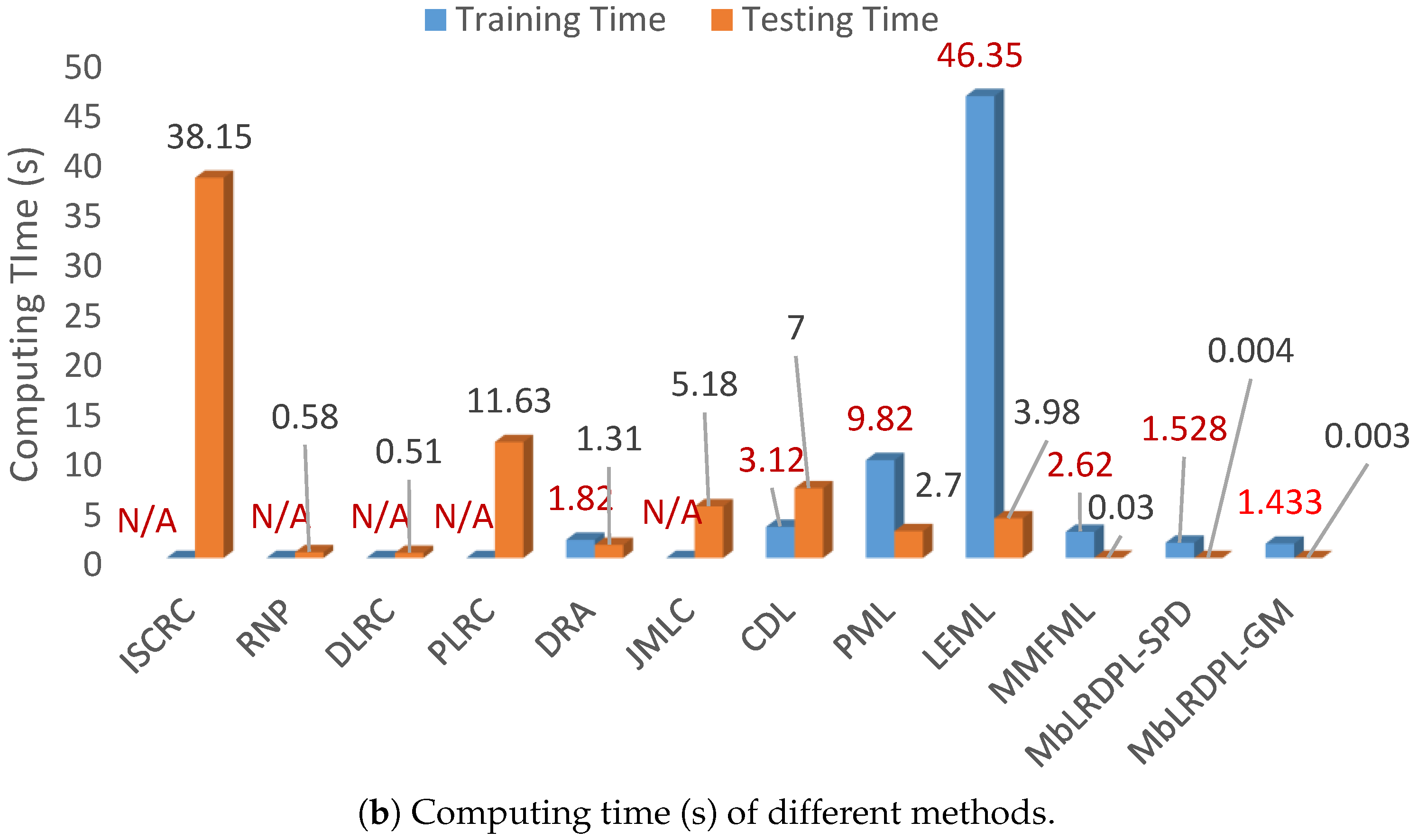
4.1. Experiments on Set-Based Video Face Recognition Task

The Honda/UCSD [26] and YouTube Celebrities (YTC) [27] datasets were used in this part of the study. The Honda dataset contains 59 video sequences, and these videos belong to 20 different categories (person). Each video contains approximately 300 to 500 frame images. In each frame, only one person exists. For fair comparison, all frames were resized to $20\times 20$ pixels. In our following experiments, one video from each category was randomly selected for training (i.e., used as a gallery video), and the rest of the videos or image sets were selected for testing (probe videos). The YTC dataset is collected from YouTube, which consists of 1910 videos, and these videos belong to 47 different categories (celebrities). Each video contains approximately hundreds of frame images; in most cases, in each frame image, only one person is present. Similar the to Honda dataset, all frame images were resized to $20\times 20$ pixels. For fair comparison, three image sets (video clips) were randomly selected from each person for training (i.e., used as the gallery videos), and six image sets were randomly selected for testing (i.e., used as the probe videos). Some illustrative samples obtained from these datasets are shown in Figure 3. All experiments were repeated 10 times, and the average experimental results are summarized in

Table 2. Classification accuracy (%), training time (Tra. Time), and testing time (Tes. Time) (seconds) of different methods on Honda and YTC datasets.

Method	Honda			YTC
	Accuracy	Tra. Time	Tes. Time	Accuracy	Tra. Time	Tes. Time
ISCRC	96.41 ± 2.24	N/A	9.36	69.31 ± 2.02	N/A	1171
RNP	96.41 ± 2.16	N/A	2.49	70.35 ± 2.44	N/A	47.12
DLRC	34.36 ± 2.15	N/A	10.15	38.37 ± 6.70	N/A	183.2
PLRC	67.53 ± 6.64	N/A	33.84	49.26 ± 2.24	N/A	3102
DRA	70.12 ± 9.22	41.23	38.33	30.19 ± 0.35	2238	2482
JMLC	100.0 ± 0.00	N/A	1.81	71.89 ± 3.13	N/A	986
CDL	100.0 ± 0.00	3.56	8.58	69.18 ± 2.65	12.58	15.69
PML	96.67 ± 2.01	5.55	3.51	66.13 ± 3.16	65.58	18.37
LEML	97.18 ± 3.32	22.34	3.90	50.60 ± 3.01	400.6	39.96
MMFML	100.0 ± 0.00	2.53	0.02	71.32 ± 4.36	18.32	0.56
DML	–	–	–	70.89 ± 9.75	10.38	0.30
MbLRDPL-SPD	100.0 ± 0.00	0.89	0.003	72.16 ± 2.44	9.73	0.47
MbLRDPL-GM	100.0 ± 0.00	0.78	0.002	71.85 ± 2.53	9.16	0.51

.

This table shows the following results: First, the proposed MbLRDPL method achieved the highest classification accuracy on both the Honda and YTC datasets. Specifically, on the Honda dataset, our method achieved 100% accuracy, which was higher than that achieved by most of the other methods used for comparison. Especially compared with PML and LEML (which also use static modeling), our proposed MbLRDPL performs much better, demonstrating that our proposed LRDPL classifier has powerful classification ability. On the YTC dataset, the proposed MbLRDPL achieved the higher accuracy of 72.16%, providing lower error than other dynamic modeling methods (ISCRC, RNP, DLRC, PLRC, DRA, and JMLC) by approximately 0.96%∼60.12%; this is a lower error than static modeling methods (CDL, PML, LEML, and MMFML) by approximately 2.93%∼43.64%; and lower error than the dynamic plus static modeling method DML by 4.36%. Second, we observed that on the Honda and YTC datasets, our MbLRDPL was much faster than the other methods in terms of training time (Tra. Time) and testing time (Tes. Time), even compared with the hash method DML. Finally, we also observed that the dynamic modeling methods were more sensitive to the size of dataset, because when using a large dataset (i.e., YTC), their computing time was considerably longer.

Since our MbLRDPL uses the dictionary learning scheme,

Table 3. Classification accuracy (%) of different dictionary learning methods on the YTC dataset.

Method	Accuracy
D-KSVD	59.20
ADDL	62.30
DDL	60.10
SLatDPL	61.90
CEBSR	66.31
MbLRDPL-SPD	72.16
MbLRDPL-GM	71.85

provides a comparison of the proposed model’s performance with that of some dictionary learning methods: 59.2% for D-KSVD [20], 62.3% for ADDL [21], 60.1% for DDL [22], 61.9% for SLatDPL [23], and 66.31% for CEBSR [5] on the YTC dataset. These results were extracted from the literature [5]. This table shows that our MbLRDPL method is substantially better than these dictionary learning methods (providing and improvement of 5.85% over the best result achieved by CDBSR), likely because the static modeling used in MbLRDPL can effectively capture the discriminative information of each image set.

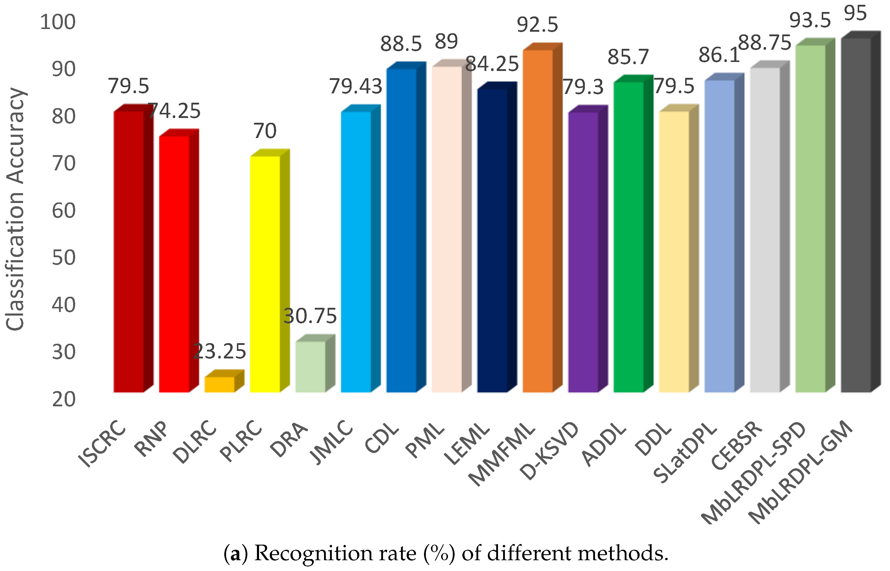
4.2. Experiments on Set-Based Object Classification Task

In this part of the study, the ETH-80 [28] dataset was used to verify the performance of the proposed method on a set-based object classification task. As shown in Figure 3c, this dataset contains 80 image sets of 8 different categories including apples, cars, cows, cups, dogs, horses, pears, and tomatoes; each category contains 10 image sets, and each image set includes 41 different views images. Each image was resized to $20\times 20$ pixels. For fair comparison, five image sets were randomly selected from each category for training (i.e., used as gallery sets), and the remaining image sets were selected for testing (i.e., used as probe sets). We repeated this process 10 times, and we report the average experimental results. The finally recognition rates and computing time of different methods are shown in Figure 4.

As shown in Figure 4a, we found that the classification accuracy of MbLRDPL was the highest, demonstrating that our proposed method can effectively deal with the object classification task. Specifically, MbLRDPL reduced the classification error of dynamic modeling methods by at least 75.61% (ISCRC) and reduced the error of static modeling methods by at least 33.33% (MMFML). These results indicate that our proposed MbLRDPL combines the advantages of both static and dynamic modeling methods, which is an observation consistent with our previous theoretical analysis. Additionally, we found that the static modeling methods performed better than the dynamic modeling methods, demonstrating that the static modeling methods are more suitable for object classification tasks. Compared with dictionary learning methods, we found that our MbLRDPL outperformed these methods by at least 6.25%, indicating that our LRDPL classifier has a more powerful classification ability. Figure 4b again shows that MbLRDPL runs much faster than the methods used for comparison, likely because the static modeling strategy can substantially reduce the number of samples, and the subsequent LRDPL classifier runs quickly by avoiding the $L_1$-norm optimization problem.

In conclusion, compared with the state-of-the-art (SOTA) methods, we observe that (a) on Honda dataset, the MbLRDPL and SOTA method JMLC both achieve 100% accuracy. However, our MbLRDPL runs much faster (about 900 times) than JMLC in terms of testing time; (b) on the YTC dataset, our MbLRDPL achieves 72.16% accuracy, reducing the errors of SOTA methods JMLC, DML and CEBSR by 0.96%, 4.36%, and 17.36%, respectively. MbLRDPL runs much faster than these SOTA methods; (c) on the ETH-80 dataset, our MbLRDPL achieves 95% accuracy, reducing the errors of SOTA methods JMLC and CEBSR by 75.69% and 55.56%, respectively. We find again that MbLRDPL runs much faster than the comparison SOTA methods.

5. Discussion

Video recognition [29,30,31] is an important direction in computer vision and video processing research. To date, many effective video recognition methods have been developed, which can be grouped into two categories: temporal–spatial- and spatial-based video recognition methods. In this study, only the spatial information of the video was considered; thus, each video was considered an unordered image set. Additionally, the video recognition task degenerated to a set-based video recognition or an image set classification task. According to the speed and accuracy requirements for image set classification tasks, our MbLRDPL uses static modeling, i.e., the covariance matrix or linear subspace, to model each image set, which considerably reduces the number of samples and accelerates the computing speed. Additionally, a new powerful classifier called LRDPL was also proposed, which not only increases the classification performance but also has a quick computing speed. Table 2 and Table 3 show the classification accuracy, training time, and testing time of different methods on the Honda and YTC datasets; the experimental results demonstrate that our proposed method obtained the highest classification accuracy with the fastest computing time (training plus testing time). In the object classification task, i.e., Figure 4, the same phenomenon can be observed. Specifically, compared with static modeling methods, our MbLRDPL provides higher classification accuracy and reduces the computing time; compared with dictionary learning methods, MbLRDPL effectively increases the accuracy. This means that the static modeling strategy can capture the discriminative features of image sets, and the LRDPL classifier has powerful classification ability.

As a fundamental video processing algorithm, the proposed MbLRDPL can be applied to many video oriented tasks, such as video-based fugitive tracking, video retrieval, video-based security monitoring, even action recognition, micro expression recognition, etc. In addition, since MbLRDPL requires less testing/inference time while maintaining recognition accuracy, it can be applied to some IoT edge devices via combining with deep features.

Since MbLRDPL uses the iterative strategy to solve the parameters, we plotted the convergence curves for the Honda and ETH-80 datasets to verify the convergence of the MbLRDPL method. The convergence curves are shown in Figure 5, which shows that our proposed MbLRDPL method can quickly converge (not more than 6 iterations), so we set the maximum iterations to 20.

6. Conclusions

In this paper, a novel manifold-based image set classification method called MbLRDPL was proposed. By combining the manifold learning and dictionary pair learning algorithms, MbLRDPL combines the advantages of both static and dynamic modeling methods: its classification accuracy is high and its computing time is fast. Extensive experimental results on both set-based video face recognition task and set-based object classification task demonstrated the superiority of the proposed method. Given its excellent performance, the proposed MbLRDPL can be applied to many video processing applications, such as video-based fugitive tracking, video retrieval, video-based security monitoring, micro expression recognition, etc. MbLRDPL can also be used in the edge computing field, because it has very fast inference speed.

The main limitations of the proposed algorithm include: (a) ignoring the importance of feature learning; (b) only one representation is used to model image set or video, while different representations can provide complementarity information; (c) when the number of frames in a video is small, its covariance matrix may be influenced by noise disturbance. Considering the limitations and applications of the research, our future studies include: (a) designing a joint learning network for combining the deep features and MbLRDPL; (b) constructing a new multi-model dictionary learning-based image set classification method; (c) improving the robustness of the covariance matrix by introducing the fractional-order embedding strategy.

References

1. Wang, R.; Guo, H.; Davis, L.S.; Dai, Q. Covariance Discriminative Learning: A Natural and Efficient Approach to Image Set Classification. In Proceedings of the 2012 IEEE Conference on Computer Vision and Pattern Recognition, Providence, RI, USA, 16–21 June 2012; pp. 2496–2503. [Google Scholar]
2. Gao, X.; Sun, Q.; Xu, H.; Wei, D.; Gao, J. Multi-model fusion metric learning for image set classification. Knowl. Based Syst. 2019, 164, 253–264. [Google Scholar] [CrossRef]
3. Zhu, P.; Zuo, W.; Zhang, L.; Shiu, S.C.K.; Zhang, D. Image Set-Based Collaborative Representation for Face Recognition. IEEE Trans. Inf. Forensics Secur. 2014, 9, 1120–1132. [Google Scholar] [CrossRef]
4. Yang, M.; Zhu, P.; Van Gool, L.; Zhang, L. Face recognition based on regularized nearest points between image sets. In Proceedings of the IEEE International Conference on Automatic Face and Gesture Recognition (FG), Shanghai, China, 22–26 April 2013; pp. 1–7. [Google Scholar]
5. Liu, D.; Liang, C.; Chen, S.; Tie, Y.; Qi, L. Auto-encoder based structured dictionary learning for visual classification. Neurocomputing 2021, 438, 34–43. [Google Scholar] [CrossRef]
6. Gu, S.; Zhang, L.; Zuo, W.; Feng, X.; Claims, A.I. Projective dictionary pair learning for pattern classification. In Proceedings of the Advances in Neural Information Processing Systems 27 (NIPS 2014), Montreal, QC, Canada, 8–13 December 2014; pp. 793–801. [Google Scholar]
7. Zhu, F.; Gao, J.; Yang, J.; Ye, N. Neighborhood linear discriminant analysis. Pattern Recognit. 2022, 123, 108422. [Google Scholar] [CrossRef]
8. Abdulrahman, A.A.; Tahir, F.S. Face recognition using enhancement discrete wavelet transform based on MATLAB. Indones. J. Electr. Eng. Comput. Sci. 2021, 23, 1128–1136. [Google Scholar] [CrossRef]
9. Zhu, F.; Zhang, W.; Chen, X.; Gao, X.; Ye, N. Large margin distribution multi-class supervised novelty detection. Expert Syst. Appl. 2023, 224, 119937. [Google Scholar] [CrossRef]
10. Mohammed, S.A.; Abdulrahman, A.A.; Tahir, F.S. Emotions Students Faces Recognition using Hybrid Deep Learning and Discrete Chebyshev Wavelet Transformations. Int. J. Math. Comput. Sci. 2022, 17, 1405–1417. [Google Scholar]
11. Tahir, F.S.; Abdulrahman, A.A.; Thanon, Z.H. Novel face detection algorithm with a mask on neural network training. Int. J. Nonlinear Anal. Appl. 2022, 13, 209–215. [Google Scholar]
12. Huang, Z.; Wang, R.; Shan, S.; Chen, X. Projection Metric Learning on Grassmann Manifold with Application to Video based Face Recognition. In Proceedings of the IEEE Conference on Computer Vision and Pattern Recognition (CVPR), Boston, MA, USA, 7–12 June 2015; pp. 140–149. [Google Scholar]
13. Huang, Z.; Wang, R.; Shan, S.; Li, X.; Chen, X. Log-Euclidean Metric Learning on Symmetric Positive Definite Manifold with Application to Image Set Classification. In Proceedings of the 32nd International Conference on Machine Learning, Lille, France, 6–11 July 2015; pp. 720–729. [Google Scholar]
14. Wei, D.; Shen, X.; Sun, Q.; Gao, X. Discrete Metric Learning for Fast Image Set Classification. IEEE Trans. Image Process. 2022, 31, 6471–6486. [Google Scholar] [CrossRef] [PubMed]
15. Gao, X.; Niu, S.; Wei, D.; Liu, X.; Wang, T.; Zhu, F.; Dong, J.; Sun, Q. Joint Metric Learning-Based Class-Specific Representation for Image Set Classification. IEEE Trans. Neural Netw. Learn. Syst. 2022, 1–15. [Google Scholar] [CrossRef] [PubMed]
16. Chen, L. Dual linear regression based classification for face cluster recognition. In Proceedings of the IEEE Conference on Computer Vision and Pattern Recognition (CVPR), Columbus, OH, USA, 23–28 June 2014; pp. 2673–2680. [Google Scholar]
17. Feng, Q.; Zhou, Y.; Lan, R. Pairwise Linear Regression Classification for Image Set Retrieval. In Proceedings of the IEEE Conference on Computer Vision and Pattern Recognition, Las Vegas, NV, USA, 26 June–1 July 2016; pp. 4865–4872. [Google Scholar]
18. Ren, C.; Luo, Y.; Xu, X.; Dai, D.; Yan, H. Discriminative Residual Analysis for Image Set Classification With Posture and Age Variations. IEEE Trans. Image Process. 2019, 29, 2875–2888. [Google Scholar] [CrossRef] [PubMed]
19. Aharon, M.; Elad, M.; Bruckstein, A. K-SVD: An algorithm for designing overcomplete dictionaries for sparse representation. IEEE Trans. Signal Process. 2006, 54, 4311–4322. [Google Scholar] [CrossRef]
20. Zhang, Q.; Li, B. Discriminative K-SVD for dictionary learning in face recognition. In Proceedings of the IEEE Computer Society Conference on Computer Vision and Pattern Recognition, San Francisco, CA, USA, 13–18 June 2010; pp. 2691–2698. [Google Scholar]
21. Zhang, Z.; Jiang, W.; Qin, J.; Zhang, L.; Li, F.; Zhang, M.; Yan, S. Jointly Learning Structured Analysis Discriminative Dictionary and Analysis Multiclass Classifier. IEEE Trans. Neural Netw. Learn. Syst. 2018, 29, 3798–3814. [Google Scholar] [CrossRef] [PubMed]
22. Mahdizadehaghdam, S.; Panahi, A.; Krim, H.; Dai, L. Deep Dictionary Learning: A PARametric NETwork Approach. IEEE Trans. Image Process. 2019, 28, 4790–4802. [Google Scholar] [CrossRef] [PubMed]
23. Zhang, Z.; Sun, Y.; Wang, Y.; Zhang, Z.; Zhang, H.; Liu, G.; Wang, M. Twin-Incoherent Self-Expressive Locality-Adaptive Latent Dictionary Pair Learning for Classification. IEEE Trans. Neural Netw. Learn. Syst. 2021, 32, 947–961. [Google Scholar] [CrossRef] [PubMed]
24. Cai, J.F.; Candès, E.J.; Shen, Z. A Singular Value Thresholding Algorithm for Matrix Completion. SIAM J. Optim. 2010, 20, 1956–1982. [Google Scholar] [CrossRef]
25. Martinez, A.M.; Kak, A.C. PCA versus LDA. IEEE Trans. Pattern Anal. Mach. Intell. 2001, 23, 228–233. [Google Scholar] [CrossRef]
26. Lee, K.C.; Ho, J.; Yang, M.H.; Kriegman, D. Videobased face recognition using probabilistic appearance manifolds. In Proceedings of the IEEE Conference on Computer Vision and Pattern Recognition, Madison, WI, USA, 18–20 June 2003; pp. 313–320. [Google Scholar]
27. Kim, M.; Kumar, S.; Pavlovic, V.; Rowley, H. Face tracking and recognition with visual constraints in real-world videos. In Proceedings of the IEEE Conference on Computer Vision and Pattern Recognition, Anchorage, AK, USA, 23–28 June 2008; pp. 1–8. [Google Scholar]
28. Leibe, B.; Schiele, B. Analyzing appearance and contour based methods for object categorization. In Proceedings of the IEEE Computer Society Conference on Computer Vision and Pattern Recognition, Madison, WI, USA, 18–20 June 2003; pp. 409–415. [Google Scholar]
29. ur Rehman, A.; Belhaouari, S.B.; Kabir, M.A.; Khan, A. On the Use of Deep Learning for Video Classification. Appl. Sci. 2023, 13, 2007. [Google Scholar] [CrossRef]
30. Liu, X.; Liu, S.; Ma, Z. A Framework for Short Video Recognition Based on Motion Estimation and Feature Curves on SPD Manifolds. Appl. Sci. 2022, 12, 4669. [Google Scholar] [CrossRef]
31. Guo, Z.; Ying, S. Whole-Body Keypoint and Skeleton Augmented RGB Networks for Video Action Recognition. Appl. Sci. 2022, 12, 6215. [Google Scholar] [CrossRef]
Figure 1. Flowchart of the proposed MbLRDPL method. A video is first modeled as a covariance matrix or linear subspace, then embedded into Euclidean tangent space: log ( C ) or Y Y T ; finally, it is fed into the proposed MbLRDPL classifier for learning discriminative dictionaries.
Applsci 13 06383 g001
Figure 2. The tree diagram of image set classification methods, and these methods can be grouped into two categories: static and dynamic modeling methods.
Applsci 13 06383 g002
Figure 3. Some examples of three datasets: (a) Honda (all images come from one video), (b) YTC (all images come from different videos), and (c) ETH-80 (the images in the first row come from different classes, whereas the images in the second row come from a same class but different image sets).
Applsci 13 06383 g003
Figure 4. The (a) recognition rate (%), and (b) computing time (s) of different methods on ETH-80 dataset. These sub-figures demonstrate that our MbLRDPL achieves the highest recognition rate (95%) with the fastest computing time.
Applsci 13 06383 g004aApplsci 13 06383 g004b
Figure 5. Convergence curves of MbLRDPL-SPD and MbLRDPL-GM on (a) Honda and (b) ETH-80 datasets. We find the proposed MbLRDPL algorithm can converge very quickly.
Applsci 13 06383 g005