Emotional State Detection Using Electroencephalogram Signals: A Genetic Algorithm Approach

Abstract

Emotion recognition based on electroencephalogram signals (EEG) has been analyzed extensively in different applications, most of them using medical-grade equipment in laboratories. The trend in human-centered artificial intelligence applications is toward using portable sensors with reduced size and improved portability that can be taken to real life scenarios, which requires systems that efficiently analyze information in real time. Currently, there is no specific set of features or specific number of electrodes defined to classify specific emotions using EEG signals, and performance may be improved with the combination of all available features but could result in high dimensionality and even worse performance; to solve the problem of high dimensionality, this paper proposes the use of genetic algorithms (GA) to automatically search the optimal subset of EEG data for emotion classification. Publicly available EEG data with 2548 features describing the waves related to different emotional states are analyzed, and then reduced to 49 features with genetic algorithms. The results show that only 49 features out of the 2548 can be sufficient to create machine learning (ML) classification models with, using algorithms such as k-nearest neighbor (KNN), random forests (RF) and artificial neural networks (ANN), obtaining results with 90.06%, 93.62% and 95.87% accuracy, respectively, which are higher than the 87.16% and 89.38% accuracy of previous works.

1. Introduction

In recent years, research in emotion detection has become increasingly important. The development of user-centric artificial intelligence-based technologies has been one of the main reasons for the growth in different application areas such as healthcare, education, entertainment, robotics, marketing, security, and surveillance. Physical expressions such as facial gestures, speech or postures have been used to identify human emotions [1,2,3,4,5,6], but in some cases, this can be ineffective because people may purposely or unconsciously mask their true feelings, which is why physiological signals can provide a more precise and objective recognition of emotions [7]. For this reason, many of the approaches in affective computing research have turned their attention to analysis through physiological signals [8,9,10,11,12,13,14,15].

Emotion recognition and human-centered research efforts have provided improved achievements thanks to the use of machine learning and deep learning algorithms [16,17]; these have evolved rapidly in recent decades and an important aspect to consider is the selection of features used to create prediction or classification models.

Genetic algorithms are optimization algorithms based on natural selection. These algorithms are executed through an iterative process of selection, crossing and mutation of chromosomes from an initial population; during this process, only the best-adapted chromosomes survive [18]. GAs have proven to be very efficient in terms of parameter optimization and dimensionality reduction [19,20,21]. In a study of emotion recognition through pulse signals and the SVM classifier, the authors evaluated the effect of using genetic algorithms for feature selection and compared the recognition rate without a selector and with a GA as the feature selector. The recognition rate increased from 52.5% to 90% when using genetic algorithms [22].

In addition, an advantage of GAs over deep network training algorithms in backpropagation is that GAs do not suffer from an evanescent gradient, as they do not use gradients for optimization. Instead, they use search techniques based on natural selection and reproduction to find optimal solutions to complex problems [23]. Algorithms that have proven to be very effective in solving classification problems are random forest, KNN and ANN, which are described in more detail in Section 2. Electroencephalogram (EEG) signals are types of physiological signals that are very sensitive to changes in emotional states. The electroencephalogram registers the potential differences of neurons when they are active, recording the electrical information from the activity of the autonomic nervous system and central nervous system [15]. One of the disadvantages of emotion analysis based on electroencephalogram signals is the fact that it involves the use of many electrodes attached to the head of the analyzed subjects, as well as a large amount of data to be analyzed. For this reason, the trend in the development of sensors for emotion recognition has been leaning towards reducing size and improving portability in order to be useful for real-life scenarios, such as wearable wireless sensors [24]. An important aspect to consider for the development of this type of sensors and systems is a reduction in the dimensionality of the data to be processed.

Previous work on EEG feature extraction has shown that there are many useful temporal and statistical features, which have proven to be effective for the recognition of different emotions. In their study, Bird J. et al. [25] explored five different feature selection methods and seven classification models, comparing their predictive ability and the number of features used. For each test, 10-fold cross validation was used to train the model. For feature selection, the best result was obtained with the OneR algorithm with 44 features selected from a set of 2100, which were used with classification models such as Naïve Bayes, Bayesian networks, random tree, support vector machine, multilayer perceptron and random forest, the last one being the most accurate with a prediction accuracy of 87.16%.

In a following study, Bird J. et al. [26] compared single and ensemble methods for classifying emotions from an EEG brainwave database, and they also compare feature selection methods such as OneR, Bayes network, information gain, and symmetrical uncertainty. From 2548 characteristics, 63 were chosen with the information gain method and their higher results of classification were found with the random forest ensemble classifier with an overall accuracy of 97.89%. The best single classifier was a deep neural network with an accuracy of 94.89%. Ten-fold cross validation was used for training the models.

In their study, Jodie Ashford and collaborators [27] classified EEG signals with an approach based on the representation of the statistical features from the signals as images. In their work, they reduce a large set of features containing 2479 features to a set only containing 256 using the algorithm of information gain measure; then, they used the resulting features to reshape them and express them as grayscale images which were then used in a deep convolutional neural network to train the data and classify the mental state of the subject with an accuracy of 89.38%. For the validation of this study, the data were split in a 70/30 ratio for training and testing, respectively.

Moreover, Liu Z. et al. [28] proposed a special feature extraction methodology using the empirical mode decomposition (EMD) domain mixed with sequence backward selection (SBS) in order to remove the reductant features. Additionally they compared different temporal windows’ lengths and the kinds of rhythms of EEG signals, the one with a length of 1 s being the one achieving the highest recognition accuracy of 86.46% in valence and 84.90% in arousal. In this work, the dataset samples were split into an 80/20 test and training ratio.

On the other hand, Xu H. and collaborators [29], using their approach, studied the effects of selecting different channels and frequency bands of EEG signals on the precision of emotion recognition. Initially, they used the discrete wavelet transform method to separate the signals into bands such as gamma, beta, alpha, and theta; then, the entropy and energy were extracted from each band as the class features. Afterwards, they evaluated channel combinations and compared them using three methods, the first one based on experience, the second based on the indirect minimal redundancy maximal relevance (mRMR-FS) algorithm, and the third one based on the direct channel selection method mRMR-CS algorithm, using each channel as a whole. In their results, of the three methods used, mRMR-CS had the best ability to reduce channels, reaching an accuracy of 79.46% and reducing the number of channels from 32 to 22.

This study proposes the use of intelligent algorithms to perform temporal and statistical feature selection from EEG brain waves related to different emotional states, with the use of genetic algorithms (GA) and KNN, RF and ANN machine learning models to classify three emotional states with improved accuracy. Section 2 discusses the materials and methods used in this research work. Section 3 provides the results. Section 4 shows the discussion, and Section 5 reports the conclusions.

The main contributions of this study are outlined below.

The proposed model enabled the dimensionality of the data to be reduced by 98.08%. Compared to similar studies, this dimensionality reduction is superior to others, and could improve the feasibility of developing specific-purpose devices for real-time applications in feature jobs.

The 49 optimal features to which the proposed model reduced the initial total of 2548 features were used to create machine learning (ML) classification models with algorithms such as k-nearest neighbor (KNN), random forests (RF) and artificial neural networks (ANN), obtaining results with 90.06%, 93.62% and 95.87% accuracy, respectively, which are higher than the 87.16% and 89.38% accuracy reported in previous works.

2. Materials and Methods

This section describes the methodology applied for data analysis using different selection and classification algorithms, as well as giving a general description of the data analyzed. Figure 1 illustrates the methodology applied, which consists of four main stages: (1) data description, (2) feature selection, (3) implementation of ML models and then (4) validation of the models. Details of the methodology are described below.

2.1. Data Description

A publicly available EEG database describing the waves related to different emotional states was used. Data from 1 male and 1 female were recorded during 3 min sessions for positive, neutral, and negative states using a Muse EEG headset. Locations TP9, AF7, AF8 and TP10 of the dry electrode were selected. Emotions were evoked using negative, positive, and neutral emotional movie clips. From the EEG brain waves, a static dataset was created using a sliding window approach. The dataset included 2548 features and 2132 observations related to an emotional state [10,25]. It was not necessary to process or remove any data.

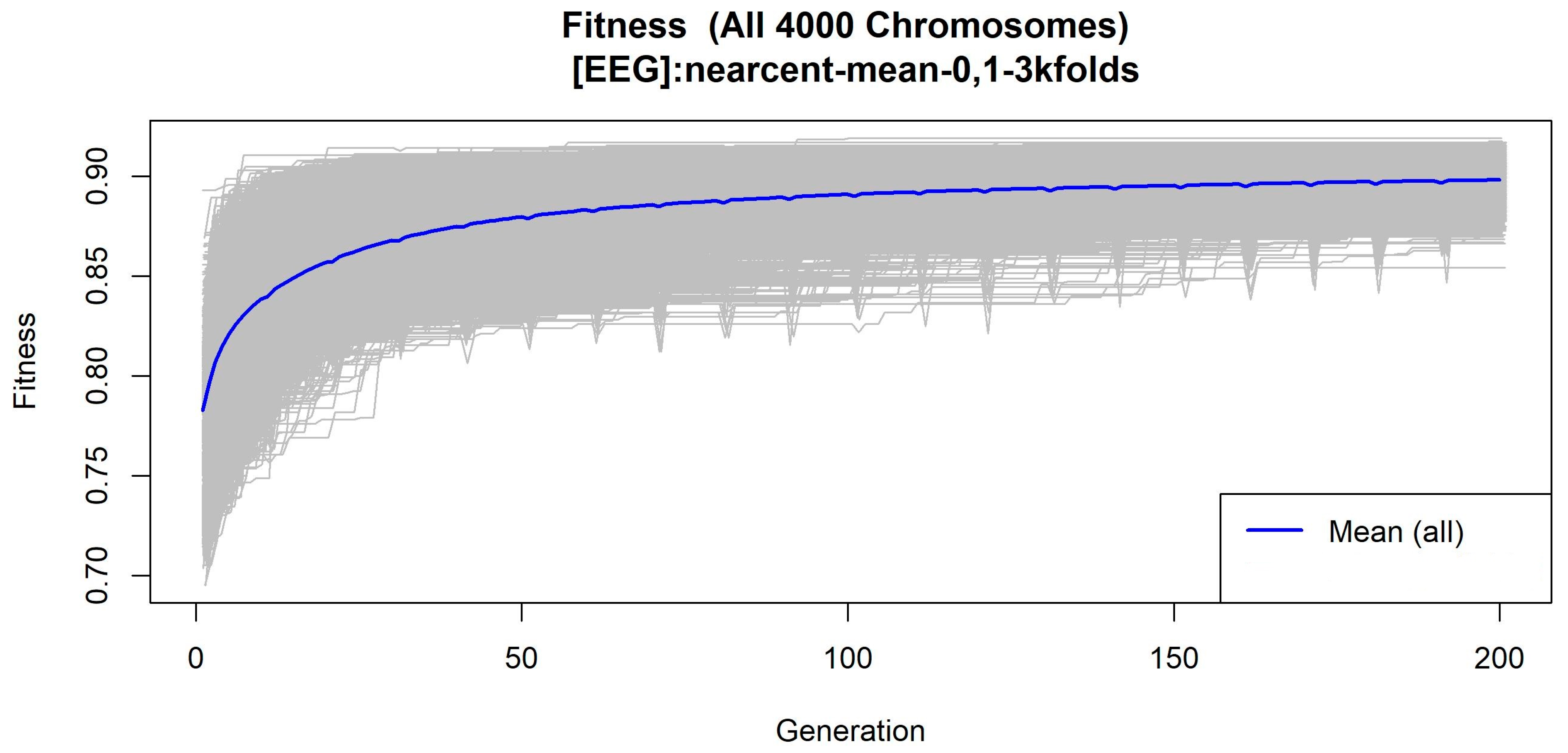
2.2. Feature Selection

The database used to carry out this work included 2548 statistical and time-dependent features to describe three mental states. All these features may have the potential to include important information to describe part of the emotional state classification problem; however, this might be computationally costly. The genetic algorithm introduced by Goldberg and Holland [30] is based on the natural selection mechanism. The algorithm’s objective is to discover the best solution for chromosome survival, with a statistical optimization approach. Genetic algorithms are based on natural behavior.

There are different types of GAs; some authors classify the variants into five main categories: real- and binary-coded, multi-objective, parallel, chaotic and hybrid [18]. The type of GA used in this study is a multi-objective statistical model-building approach with a specific search strategy for variable selection. The general operation of the GA is based on the random creation of a population called (Y) of n chromosomes; the fitness of each chromosome in the population is evaluated, according to this evaluation two chromosomes, C1 and C2 are selected, and a crossover operator with crossover probability (Cp) is applied to those chromosomes C1 and C2 to produce an offspring, O. Then, a mutation operator with mutation probability (Mp) is applied on the offspring O to generate O′. Finally, the offspring O′ is placed in the new population. From here, the selection, crossover and mutation operations are repeated iteratively until the new population is complete. Figure 2 represents the GA flow chart with the following listed steps:

• Step 1: creation of a random initial population of chromosomes, which in this case are sets of 5 genes or features.
• Step 2: consisting in the evaluation of the capability of the chromosomes to predict the different emotional states, with this creating a statistical model, the GA assigns a score to each chromosome, and this score is proportional to the resulting accuracy of the model. In this study, the nearest centroid classifier is used in the model.
• Step 3: if the score in the previous step is higher than that of the defined fitness goal, the chromosome is selected; if it is not, the process continues.
• Step 4: the chromosomes best suited to the problem are replicated; the higher the score, the bigger the offspring.
• Step 5: the crossover consists of a recombination of pairs of good chromosomes from the genetic information of the replicated parents.
• Step 6: the mutations created in Step 5 are now included in the new population, allowing new genes to be included in the chromosomes.
• Step 7: the process is repeated from Step 2 onwards until a solution is found; each cycle from Step 4 to Step 6 is referred to as a generation.

Figure 2. GA procedure flow chart.

Figure 2. GA procedure flow chart.

In this study, an R package named GALGO is used [30,31].

Table 1. GALGO parameters.

Parameter	Value
Classification method	Nearcent
Chromosome size	5
Solutions	4000
Generations	200
Goal fitness	1

describes the parameters selected for the GALGO analysis. The classification method selected was nearest centroid, which is a very simple and fast classifier capable of classifying data without feature selection and is also computationally inexpensive.

2.3. ML Model Implementation

After the feature selection process, in order to avoid bias towards a specific algorithm, three different classification algorithms were implemented to evaluate the efficiency of the models; for this stage, random forest, KNN and ANN were used, and these models are described below. The experiments in this study were carried out on a Dell G15 Ryzer Edition machine with a Windows 11 operating system. The models and methodologies were implemented in R, and the open source software was validated by the scientific community. The libraries used for the ML models were “caret” and “neuralnet”.

2.3.1. Random Forest

Random forest is a complex machine learning algorithm that combines the results of different decision trees in parallel, as shown in Figure 3, on different subsamples of datasets using the majority or average voting for the final result to perform a classification or regression problem [32].

2.3.2. k-Nearest Neighbor

Many classification and regression problems are described with the k-nearest neighbor algorithm, a supervised statistical algorithm which measures the similarity of the training set and the test set; it defines the class of an object based on the level of similarity between it and the training examples. The first step is to select a sample for training and the second step is to define “k”, the number of neighbors; the higher the number of k, the higher the accuracy. The algorithm utilizes the Euclidean distance formula in order to find the k-nearest samples of the training data for each test data as shown in Equation (1). The training samples that each class has are counted and compared with “k”, and then the class of the test event is selected as the most popular class from the k training samples [33].

$$D\left(A,B\right)=\sqrt{{\sum }_{i=1}^n{\left(a_i-b_i\right)}^2}$$

(1)

where A is the feature vector of a new sample, B is the feature vector of a single training sample, n is the total number of features used for prediction, and a and b are the i-th components of A and B, respectively.

2.3.3. Artificial Neural Networks

ANNs are a machine learning method used for classification or prediction that emulates learning from prior information, such as that from neurons in the human brain. A neural network is defined by the connections between the neurons, while the training algorithm is used to determine the weights on the connections, and the activation function, e.g., the logistic sigmoid function shown in Equation (2). Figure 4 shows the structure of an ANN, with three essential parts: the input layers, hidden layers and output layer. The data are received in the input layer and then used in the hidden layers to perform mathematical calculations and recognize patterns. The result obtained from the calculation is the output layer [34]

$$f\left(x\right)=\frac{1}{1+e^{-x}},$$

(2)

2.4. Model Validation

To evaluate the results of the algorithms, the database was split in a 75:25 ratio. The models were trained with 75% of the data and the remaining 25% was used to test them. The performance of the models in emotion recognition was evaluated using the following statistical metrics: overall accuracy, confusion matrix, sensitivity, and specificity. From the information provided by the confusion matrix shown in

Table 2. Confusion matrix.

	Actually Positive	Actually Negative
Predicted Positive	True positives (TP)	False positives (FP)
Predicted Negative	False negatives (FN)	True negatives (TN)

, sensitivity, specificity and overall accuracy can be computed. Overall accuracy as shown in Equation (3) denotes the proportion of correctly predicted classifications over the total number of instances; in some cases, this could be a deceptive measure, and for this reason sensitivity and specificity are computed. Sensitivity describes the capability of an algorithm to predict a positive class when the actual one is positive, and specificity describes the capability of an algorithm to not predict a positive class when the actual one is not positive [35].

Overall Accuracy = TP + TN/(TP + TN + FP + FN)

(3)

Sensitivity = TP/(TP + FN)

(4)

Specificity = TN/(TN + FP)

(5)

3. Results

With the results of the GA analysis in the R software (Version 3.6.3), Figure 5 shows the fitness scores over generations; the ordinate axis indicates the fitness score, and the abscissa axis represents the generations. This graph represents the chromosomes’ capacity to accurately detect each emotional state, with the blue line indicating all models’ mean fitness. As can be deduced from Figure 5, after 150 generations, there was no appreciable change in the fitness score, demonstrating that the previously established value of 200 was congruent.

Figure 6 showing the Gene Rank Stability graph displays the ranked stability of the genes showing the stability of the features in the models in order. The first features are the most stable and their color is solid, which means these features contribute more to the classification.

After ranking the most significant features, the forward selection method outputs 49 features, as shown in Figure 7. The ordinate axis indicates the accuracy in terms of classification, and the abscissa axis presents the features in order of importance, while the black line is the best-performing model which in this case is model number 23 with an accuracy of 0.9019. With regard to this, it could be said that the 49 features listed in

Table 3. Resulting features.

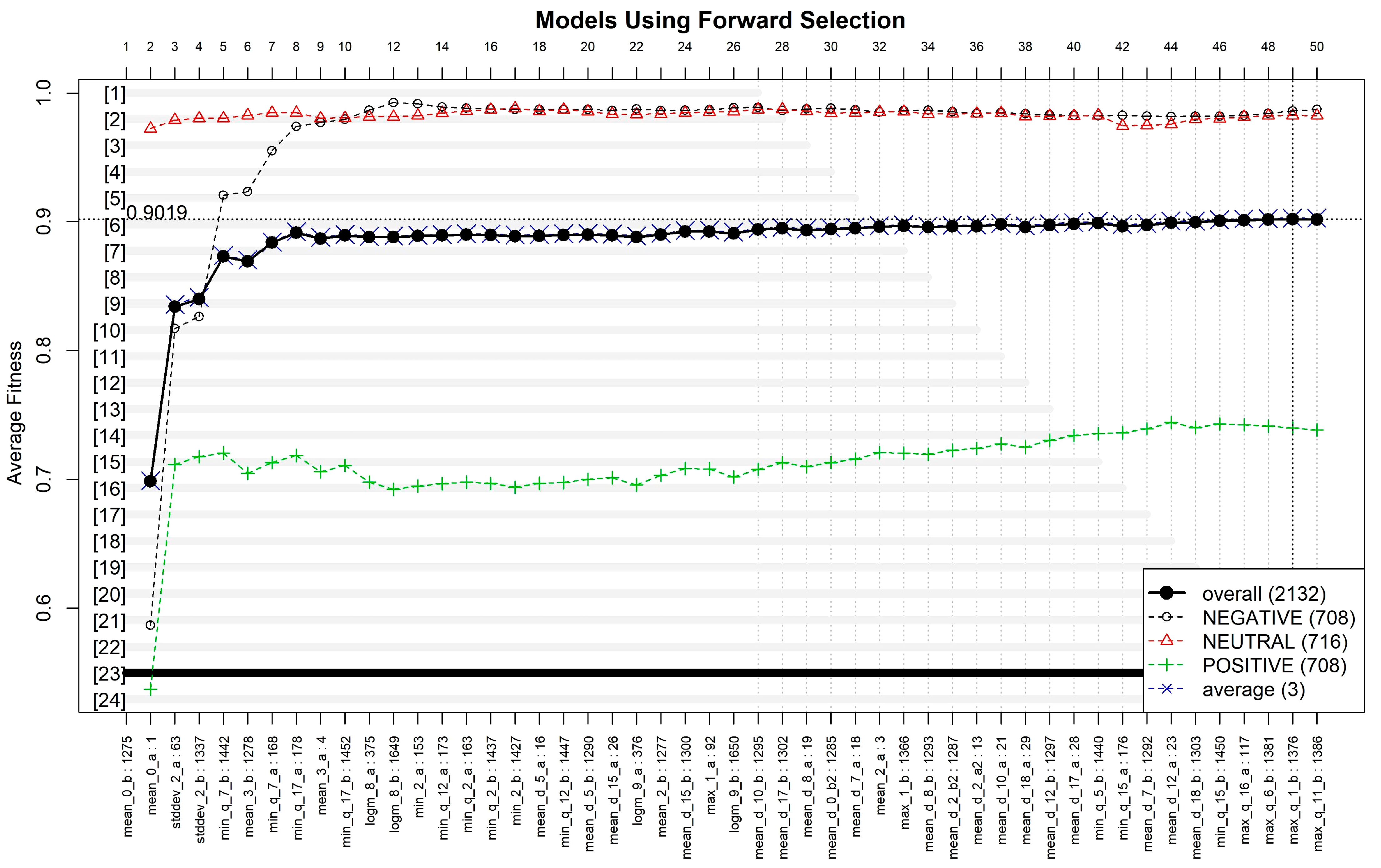
Model 23′s Features

“mean_0_b”, “mean_0_a”, “stddev_2_a”, “stddev_2_b”, “min_q_7_b”, “mean_3_b”, “min_q_7_a”, “min_q_17_a”, “mean_3_a”, “min_q_17_b”, “logm_8_a”, “logm_8_b”, “min_2_a”, “min_q_12_a”, “min_q_2_a”, “min_q_2_b”, “min_2_b”, “mean_d_5_a”, “min_q_12_b”, “mean_d_5_b”, “mean_d_15_a”, “logm_9_a”, “mean_2_b”, “mean_d_15_b”, “max_1_a”, “logm_9_b”, “mean_d_10_b”, “mean_d_17_b”, “mean_d_8_a”, “mean_d_0_b2”, “mean_d_7_a”, “mean_2_a”, “max_1_b”, “mean_d_8_b”, “mean_d_2_b2”, “mean_d_2_a2”, “mean_d_10_a”, “mean_d_18_a”, “mean_d_12_b”, “mean_d_17_a”, “min_q_5_b”, “min_q_15_a”, “mean_d_7_b”, “mean_d_12_a”, “mean_d_18_b”, “min_q_15_b”, “max_q_16_a”, “max_q_6_b”, “max_q_1_b”.

GA-selected features listed in order of importance according to their rank from Figure 6.

include important information from the EEG signal with which to classify the emotional states, and this represent a 98% reduction in the total number of features. Figure 8 shows the data distribution related to each emotional state from the 49 selected features.

With the 49 features selected within the best-accuracy model during the genetic algorithm’s implementation, the performance of three machine learning methods was assessed for the prediction of the negative, neutral, and positive emotional states in the test proportion of the data. The algorithms used are; KNN, RF and ANN.

Table 4. ML model’s overall accuracy for the test data.

	KNN	RF	ANN
Overall Accuracy	90.43%	93.43%	95.87%

show the Overall accuracy of the three models. The results have shown a higher overall accuracy of ANN model over KNN and RF. For more detailed information the Confusion Matrixes are presented in

Table 5. KNN, RF and ANN model’s confusion matrix for the test data.

	KNN	Reference				RF	Reference				ANN	Reference
		Neg.	Neu.	Pos.			Neg.	Neu.	Pos.			Neg.	Neu.	Pos.
Prediction	Neg.	160	10	1	Prediction	Neg.	170	8	0	Prediction	Neg.	166	5	6
	Neu.	0	184	1		Neu.	0	170	0		Neu.	0	177	2
	Pos.	22	17	138		Pos.	1	26	150		Pos.	4	5	168

. KNN, RF and ANN Model’s confusion matrix for the test data.

Table 5 shows the confusion matrixes for the three models. In the case of KNN, from this visualization, it can be inferred that the best performance of the model is for classifying the positive class, since according to the reference positive column, only two instances were wrongly predicted which correspond to just 1.4% of the total positive instances, and this can be confirmed with the sensitivity result of 0.9857 shown in

Table 6. KNN, RF and ANN model’s sensitivity and specificity for the test data.

	Neg.	Neu.	Pos.
KNN Sensitivity	0.8791	0.8720	0.9857
RF Sensitivity	0.9942	0.8396	1.0000
ANN Sensitivity	0.9765	0.9465	0.9545
	Neg.	Neu.	Pos.
KNN Specificity	0.9687	0.9969	0.9008
RF Specificity	0.9779	1.0000	0.9295
ANN Specificity	0.9697	0.9942	0.9748

. In contrast, in the negative and neutral classes, 22 and 27 predictions were wrong, which correspond to 12.08% and 12.7% of the total negative and neutral instances.

In the same way, the confusion matrix of the Random Forest model shows its best performance classifying the positive class with 0% of mistakes, and it shows a very good performance classifying the negative class, since there was only 1 instance wrongly predicted which corresponds to only 0.58% of the total Negative classes. In contrast, the neutral class has 34 predictions wrongly classified out of 204, which corresponds to the 16% of the total Neutral classes. These results can be correlated with their corresponding values of sensitivity and specificity shown in Table 6.

In the case of the ANN model, the overall accuracy of which was the highest, it can be said that its best performance was for recognizing the negative emotional state, since there were only four instances wrongly predicted. In the second place was its performance for the positive class with eight instances being wrongly predicted. Finally, in the third place was its performance for the neutral class with ten instances being wrongly predicted. In overall terms, ANN had the best performance, and this can be correlated with the corresponding values of sensitivity and specificity, where all results are over 0.9465 and close to 1, as shown in Table 6.

4. Discussion

In this analysis, we developed a GA model based on the nearest center classification method, in order to reduce the data dimensionality from a publicly available EEG signal dataset to classify three emotional states. After reducing the data from 2548 features to only 49 features and reaching an accuracy of 90.19%, three ML classification algorithms (KNN, RF and ANN) were evaluated to classify negative, neutral, and positive emotional states. The results show that the 49 features selected by the GA from the total of 2548 features are sufficient to create ML classification models with, obtaining results of 90.43% and 93.43% and 95.87% for KNN, RF and ANN, respectively, the last one being the most accurate.

Table 7. Comparison of this study with previous similar studies.

Autor’s	Overall Accuracy	Observations
This Study	95.87%	49 out of 2548 features selected with genetic algorithms and ANN ML model for classification.
Bird J. et al. [25]	87.16%	44 out of 2100 features were used with classification models such as Bayesian networks, support vector machine and random forest, the last one being the most accurate.
Bird J. et al. [26]	97.89%	63 out of 2548 features selected via information gain measurement. Classification method: random forest ensemble classifier.
Ashford et al. [27]	89.38%	256 out of 2479 features selected based on information gain measurement from gray-scale image representation of statistical features. Classification method: deep convolutional neural network.

shows a comparison of this study with previous studies of the same database using different methodologies to improve feature selection and emotional state recognition via EEG signals. Although our results present the second highest overall performance, as shown in Table 7, our work uses 14 fewer features than the report [26] which has 2.02 points higher overall performance. This means that in terms of dimensionality reduction our method is still better.

Furthermore, considering Figure 7 (models using the forward selection), it can be observed that with only the first eight features, listed as mean_0_b, mean_0_a, stddev_2_a, stddev_2_b, min_q_7_b, mean_3_b, min_q_7_a and min_q_17_a in the graph, very similar performances close to 90% accuracy could be achieved with only 0.31% of the total 2548 features contained in the database, which is the percentage represented by these eight features. This is a much greater reduction in the dimensionality of data than that previously reported in similar studies.

Moreover, in order compare our methodology with standard method for feature selection in Python, called sequential feature selection (SFS) [36], an additional experiment was performed. The SFS algorithm starts by selecting an initial set of features and evaluating their predictive power. The algorithm then proceeds iteratively, evaluating the performance of the model with an increasing number of features, adding or removing one feature at a time, until the desired number of features is reached or no further improvement in performance is observed. To compare our proposed feature selection methodology, GALGO, to SFS, the same number of optimal features (49) were set as the parameter for the SFS methodology, and the resulting SFS features were tested with the same ML models as those used in our study. As shown in

Table 8. GA and SFS feature selection comparison.

GA Feature Selection	KNN	RF	ANN
Overall Accuracy	90.43%	93.43%	95.87%
Sequential Feature Selection	KNN	RF	ANN
Overall Accuracy	74.11%	92.68%	84.98%

, all the overall accuracies of the ML models analyzed with the selected features from the SFS model were below our accuracies, so it can be said that the multi-objective genetic algorithms outperform SFS. For this test, the Python library used was SciKit-Learn, version 0.24 [37].

5. Conclusions

In this work, a multi-objective GA statistical model with a specific search strategy for variable selection was proposed and tested in a high-dimensional EEG signal database for emotional classification.

The proposed model allowed a reduction in the dimensionality of the data of 98.08%. This model, compared to that used in similar studies, outperforms the dimensionality reduction sought, which could enhance the feasibility of developing specific-purpose devices for real-time applications in future works.

The proposed model reduced the 2548 features describing the waves related to different emotional states, to only 49 optimal features, which were used to create machine learning (ML) classification models with algorithms such as k-nearest neighbor (KNN), random forests (RF) and artificial neural networks (ANN), obtaining results with 90.06%, 93.62% and 95.87% accuracy, respectively, which are higher than the 87.16% and 89.38% accuracy of previous works.

Furthermore, according to our forward selection analysis, it can be inferred that by sacrificing a little accuracy without going below 90%, emotional states could be described with only eight features or 0.31% of the total of 2548 features contained in the database used, which was a reduction unlike any other published in similar studies.

Additionally, a comparison was made between the selection method used and the widely validated method: sequential feature selection of the SciKit-Learn library (https://scikit-learn.org/stable/, accessed on 9 May 2023). From this comparison, it can be observed that GALGO has better results. As shown in Table 8, the three algorithms that used the features selected using GALGO obtained better results than the algorithms that used the features selected with SFS did, so we can validate the feature selection methodology proposed in this research and affirm that GALGO works very well and obtains better models than the traditional ones do.

The proposed methodology generated a model with a promising approach for detecting emotions in real time using only 49 features extracted from EEG signals. With the increasing interest in affective computing and the need for non-invasive methods of emotion recognition, this model could have significant applications in fields such as psychology, neuroscience, and human–computer interactions. The potential for real-time emotion detection represents a significant step forward in our understanding of the complex relationship between brain activity and emotions.

In future work, we plan to create our own databases in order to increase the number of test subjects and validate the architecture with more support. Additionally, the research can be further extended by focusing on identifying specific features and electrodes describing each class of emotion to improve the feasibility of developing purpose-built devices for real-time applications.

References

- Kim, J.H.; Poulose, A.; Han, D.S. The Extensive Usage of the Facial Image Threshing Machine for Facial Emotion Recognition Performance. Sensors 2021, 21, 2026. [Google Scholar] [CrossRef] [PubMed]
- Canal, F.Z.; Müller, T.R.; Matias, J.C.; Scotton, G.G.; de Sa Junior, A.R.; Pozzebon, E.; Sobieranski, A.C. A Survey on Facial Emotion Recognition Techniques: A State-of-the-Art Literature Review. Inf. Sci. 2022, 582, 593–617. [Google Scholar] [CrossRef]
- Karnati, M.; Seal, A.; Bhattacharjee, D.; Yazidi, A.; Krejcar, O. Understanding Deep Learning Techniques for Recognition of Human Emotions Using Facial Expressions: A Comprehensive Survey. IEEE Trans. Instrum. Meas. 2023, 72, 1–31. [Google Scholar] [CrossRef]
- Kakuba, S.; Poulose, A.; Han, D.S. Deep Learning-Based Speech Emotion Recognition Using Multi-Level Fusion of Concurrent Features. IEEE Access 2022, 10, 125538–125551. [Google Scholar] [CrossRef]
- Yan, Y.; Shen, X. Research on Speech Emotion Recognition Based on AA-CBGRU Network. Electronics 2022, 11, 1409. [Google Scholar] [CrossRef]
- Soman, G.; Vivek, M.V.; Judy, M.V.; Papageorgiou, E.; Gerogiannis, V.C. Precision-Based Weighted Blending Distributed Ensemble Model for Emotion Classification. Algorithms 2022, 15, 55. [Google Scholar] [CrossRef]
- Lin, W.; Li, C. Review of Studies on Emotion Recognition and Judgment Based on Physiological Signals. Appl. Sci. 2023, 13, 2573. [Google Scholar] [CrossRef]
- Awais, M.; Raza, M.; Singh, N.; Bashir, K.; Manzoor, U.; Islam, S.U.; Rodrigues, J.J.P.C. LSTM-Based Emotion Detection Using Physiological Signals: IoT Framework for Healthcare and Distance Learning in COVID-19. IEEE Internet Things J. 2021, 8, 16863–16871. [Google Scholar] [CrossRef]
- AlZoubi, O.; D’Mello, S.K.; Calvo, R.A. Detecting Naturalistic Expressions of Nonbasic Affect Using Physiological Signals. IEEE Trans. Affect. Comput. 2012, 3, 298–310. [Google Scholar] [CrossRef]
- Albraikan, A.; Tobon, D.P.; El Saddik, A. Toward User-Independent Emotion Recognition Using Physiological Signals. IEEE Sens. J. 2019, 19, 8402–8412. [Google Scholar] [CrossRef]
- Chao, H.; Dong, L. Emotion Recognition Using Three-Dimensional Feature and Convolutional Neural Network from Multichannel EEG Signals. IEEE Sens. J. 2021, 21, 2024–2034. [Google Scholar] [CrossRef]
- Egger, M.; Ley, M.; Hanke, S. Emotion Recognition from Physiological Signal Analysis: A Review. Electron. Notes Theor. Comput. Sci. 2019, 343, 35–55. [Google Scholar] [CrossRef]
- Santamaria-Granados, L.; Munoz-Organero, M.; Ramirez-Gonzalez, G.; Abdulhay, E.; Arunkumar, N. Using Deep Convolutional Neural Network for Emotion Detection on a Physiological Signals Dataset (AMIGOS). IEEE Access 2019, 7, 57–67. [Google Scholar] [CrossRef]
- Saganowski, S.; Perz, B.; Polak, A.; Kazienko, P. Emotion Recognition for Everyday Life Using Physiological Signals from Wearables: A Systematic Literature Review. IEEE Trans. Affect. Comput. 2022, 12, 1. [Google Scholar] [CrossRef]
- Bota, P.J.; Wang, C.; Fred, A.L.N.; Placido Da Silva, H. A Review, Current Challenges, and Future Possibilities on Emotion Recognition Using Machine Learning and Physiological Signals. IEEE Access 2019, 7, 140990–141020. [Google Scholar] [CrossRef]
- Sepúlveda, A.; Castillo, F.; Palma, C.; Rodriguez-Fernandez, M. Emotion Recognition from ECG Signals Using Wavelet Scattering and Machine Learning. Appl. Sci. 2021, 11, 4945. [Google Scholar] [CrossRef]
- Sedik, A.; Marey, M.; Mostafa, H. WFT-Fati-Dec: Enhanced Fatigue Detection AI System Based on Wavelet Denoising and Fourier Transform. Appl. Sci. 2023, 13, 2785. [Google Scholar] [CrossRef]
- Katoch, S.; Chauhan, S.S.; Kumar, V. A Review on Genetic Algorithm: Past, Present, and Future. Multimed. Tools Appl. 2021, 80, 8091–8126. [Google Scholar] [CrossRef]
- Salih, O.; Duffy, K.J. Optimization Convolutional Neural Network for Automatic Skin Lesion Diagnosis Using a Genetic Algorithm. Appl. Sci. 2023, 13, 3248. [Google Scholar] [CrossRef]
- Al-Tawil, M.; Mahafzah, B.A.; Al Tawil, A.; Aljarah, I. Bio-Inspired Machine Learning Approach to Type 2 Diabetes Detection. Symmetry 2023, 15, 764. [Google Scholar] [CrossRef]
- Lin, Z.-H.; Woo, J.-C.; Luo, F.; Chen, Y.-T. Research on Sound Imagery of Electric Shavers Based on Kansei Engineering and Multiple Artificial Neural Networks. Appl. Sci. 2022, 12, 10329. [Google Scholar] [CrossRef]
- Yu, S.-N.; Chen, S.-F. Emotion State Identification Based on Heart Rate Variability and Genetic Algorithm. In Proceedings of the 2015 37th Annual International Conference of the IEEE Engineering in Medicine and Biology Society (EMBC), Milan, Italy, 25–29 August 2015; IEEE: Piscataway, NJ, USA, 2015; pp. 538–541. [Google Scholar]
- Abuqaddom, I.; Mahafzah, B.A.; Faris, H. Oriented Stochastic Loss Descent Algorithm to Train Very Deep Multi-Layer Neural Networks without Vanishing Gradients. Knowl.-Based Syst. 2021, 230, 107391. [Google Scholar] [CrossRef]
- Ragot, M.; Martin, N.; Em, S.; Pallamin, N.; Diverrez, J.-M. Emotion Recognition Using Physiological Signals: Laboratory vs. Wearable Sensors. In Proceedings of the AHFE 2017 International Conference on Advances in Human Factors and Wearable Technologies, Los Angeles, CA, USA, 17–21 July 2017; pp. 15–22. [Google Scholar]
- Bird, J.J.; Manso, L.J.; Ribeiro, E.P.; Ekart, A.; Faria, D.R. A Study on Mental State Classification Using EEG-Based Brain-Machine Interface. In Proceedings of the 2018 International Conference on Intelligent Systems (IS), Funchal, Portugal, 25–27 September 2018; IEEE: Piscataway, NJ, USA, 2018; pp. 795–800. [Google Scholar]
- Bird, J.J.; Ekart, A.; Buckingham, C.D.; Faria, D.R. Mental Emotional Sentiment Classification with an Eeg-Based Brain-Machine Interface. In Proceedings of the International Conference on Digital Image and Signal Processing, Oxford, UK, 29–30 April 2019. [Google Scholar]
- Ashford, J.; Bird, J.J.; Campelo, F.; Faria, D.R. Classification of EEG Signals Based on Image Representation of Statistical Features. In Advances in Computational Intelligence Systems: Contributions Presented at the 19th UK Workshop on Computational Intelligence, Portsmouth, UK, 4–6 September 2019; Springer: Cham, Switzerland, 2020; pp. 449–460. [Google Scholar]
- Liu, Z.T.; Xie, Q.; Wu, M.; Cao, W.H.; Li, D.Y.; Li, S.H. Electroencephalogram Emotion Recognition Based on Empirical Mode Decomposition and Optimal Feature Selection. IEEE Trans. Cogn. Dev. Syst. 2019, 11, 517–526. [Google Scholar] [CrossRef]
- Xu, H.; Wang, X.; Li, W.; Wang, H.; Bi, Q. Research on EEG Channel Selection Method for Emotion Recognition. In Proceedings of the IEEE International Conference on Robotics and Biomimetics, ROBIO 2019, Dali, China, 6–8 December 2019; pp. 2528–2535. [Google Scholar] [CrossRef]
- Goldberg, D.E.; Holland, J.H. Genetic Algorithms and Machine Learning. Mach. Learn. 1988, 3, 95–99. [Google Scholar] [CrossRef]
- Trevino, V.; Falciani, F. GALGO: An R Package for Multivariate Variable Selection Using Genetic Algorithms. Bioinformatics 2006, 22, 1154–1156. [Google Scholar] [CrossRef]
- Sarker, I.H. Machine Learning: Algorithms, Real-World Applications and Research Directions. SN Comput. Sci. 2021, 2, 160. [Google Scholar] [CrossRef]
- Houssein, E.H.; Hammad, A.; Ali, A.A. Human Emotion Recognition from EEG-Based Brain–Computer Interface Using Machine Learning: A Comprehensive Review. Neural Comput. Appl. 2022, 34, 12527–12557. [Google Scholar] [CrossRef]
- Fausett, L.V. Fundamentals of Neural Networks: Architectures, Algorithms and Applications; Pearson Education: Chennai, India, 2006. [Google Scholar]
- Irizarry, R.A. Introduction to Data Science: Data Analysis and Prediction Algorithms with R; CRC Press: Boca Raton, FL, USA, 2019. [Google Scholar]
- Pilnenskiy, N.; Smetannikov, I. Feature Selection Algorithms as One of the Python Data Analytical Tools. Future Internet 2020, 12, 54. [Google Scholar] [CrossRef]
- Fabian, P. Scikit-Learn: Machine Learning in Python. J. Mach. Learn. Res. 2011, 12, 2825. [Google Scholar]