Explainable Mortality Prediction Model for Congestive Heart Failure with Nature-Based Feature Selection Method

Abstract

A mortality prediction model can be a great tool to assist physicians in decision making in the intensive care unit (ICU) in order to ensure optimal allocation of ICU resources according to the patient’s health conditions. The entire world witnessed a severe ICU patient capacity crisis a few years ago during the COVID-19 pandemic. Various widely utilized machine learning (ML) models in this research field can provide poor performance due to a lack of proper feature selection. Despite the fact that nature-based algorithms in other sectors perform well for feature selection, no comparative study on the performance of nature-based algorithms in feature selection has been conducted in the ICU mortality prediction field. Therefore, in this research, a comparison of the performance of ML models with and without feature selection was performed. In addition, explainable artificial intelligence (AI) was used to examine the contribution of features to the decision-making process. Explainable AI focuses on establishing transparency and traceability for statistical black-box machine learning techniques. Explainable AI is essential in the medical industry to foster public confidence and trust in machine learning model predictions. Three nature-based algorithms, namely the flower pollination algorithm (FPA), particle swarm algorithm (PSO), and genetic algorithm (GA), were used in this study. For the classification job, the most widely used and diversified classifiers from the literature were used, including logistic regression (LR), decision tree (DT) classifier, the gradient boosting (GB) algorithm, and the random forest (RF) algorithm. The Medical Information Mart for Intensive Care III (MIMIC-III) dataset was used to collect data on heart failure patients. On the MIMIC-III dataset, it was discovered that feature selection significantly improved the performance of the described ML models. Without applying any feature selection process on the MIMIC-III heart failure patient dataset, the accuracy of the four mentioned ML models, namely LR, DT, RF, and GB was 69.9%, 82.5%, 90.6%, and 91.0%, respectively, whereas with feature selection in combination with the FPA, the accuracy increased to 71.6%, 84.8%, 92.8%, and 91.1%, respectively, for the same dataset. Again, the FPA showed the highest area under the receiver operating characteristic (AUROC) value of 83.0% with the RF algorithm among all other algorithms utilized in this study. Thus, it can be concluded that the use of feature selection with FPA has a profound impact on the outcome of ML models. Shapley additive explanation (SHAP) was used in this study to interpret the ML models. SHAP was used in this study because it offers mathematical assurances for the precision and consistency of explanations. It is trustworthy and suitable for both local and global explanations. It was found that the features that were selected by SHAP as most important were also most common with the features selected by the FPA. Therefore, we hope that this study will help physicians to predict ICU mortality for heart failure patients with a limited number of features and with high accuracy.

1. Introduction

The intensive care unit (ICU) is a hospital department that provides critical care, nursing, and support to patients who are severely sick [1]. When a patient’s serious health concerns necessitate close monitoring, he or she is admitted to the ICU. The ICU is more expensive than ordinary hospital care, since it provides additional health support and uses expensive medical equipment. From the standpoint of Bangladesh, a crisis in the ICU exists in comparison to the overall population, as we saw during the COVID-19 event. Mortality prediction in the ICU might be a helpful choice for ensuring the optimum utilization of ICU resources. This prediction model can also assist clinicians in making decisions prior to assigning ICU services to patients. Those with more serious conditions require additional ICU attention. Patients at low risk, on the other hand, may be discharged from the ICU to make room for dangerously ill incoming patients. Furthermore, in the event of an ICU crisis, the mortality prediction model can assist in identifying patients with a high chance of survival and prioritizing them.

In this study, a mortality prediction model is proposed for use in the ICU, with a focus on heart failure patients. Heart failure is a serious heart disorder in which the heart is unable to efficiently pump blood around the body. According to the American Heart Association, the number of persons diagnosed with heart failure is on the rise, with a 46 percent increase expected by 2030, resulting in over 8 million people suffering from the disease [2]. According to a previous study, one out of every five patients with heart failure admitted to a hospital in the United States is admitted to an ICU, a resource-intense environment that accounts for 20–35 percent of overall hospital costs [3]. As a result, as the number of patients with heart failure rises, proper ICU distribution among those patients becomes increasingly crucial. The data on heart failure patients used in this study was gathered from the Medical Information Mart for Intensive Care III (MIMIC-III) dataset [4], which is a publicly available dataset that contains deidentified health data from thousands of ICU admissions. The demographic information, vital signs of heart failure patients, some laboratory variables, and comorbidities were all included in the dataset of heart failure patients used in this study.

Background research in the field of ICU mortality prediction demonstrates that there is still room for improvement and development by carrying out comparative studies with feature selection using nature-based algorithms vs. no feature selection. Likewise, research can be extended using explainable AI to determine which features predominate in the prediction process for patients with heart failure in order to make the models more transparent and trustworthy. We conducted our research using these points as research gaps.

In this research, we compared the performance of machine learning (ML) models with and without feature selection. Feature selection aids in reducing the curse of dimensionality, as well as speeding up and simplifying the ML method. It can also improve an ML model’s performance. Analysis of background studies [5,6,7,8,9] reveals that nature-based algorithms, namely the flower pollination algorithm (FPA) [10], the Particle swarm algorithm (PSO) [11], and the genetic algorithm (GA) [12] are three of the most effective and utilized algorithms in selecting features. Therefore, in this study, we used certain nature-based algorithms for feature selection. Three nature-based feature selection algorithms, namely the FPA, PSO, and GA, were utilized in this research. Following feature selection, the classification job was carried out using four popular ML models: logistic regression (LR) [13], gradient boosting (GB) [14], random forest (RF) [15], and decision tree (DT) [16]. Finally, the performance of the ML models was compared in terms of accuracy and area under the receiver operating characteristic (AUROC) to determine whether feature selection had an impact.

Explainable AI [17] was employed to interpret the ML models’ decisions. Explainable artificial intelligence (AI) is a set of techniques and strategies that allow humans to understand and trust the results and output of ML algorithms. For the purpose of explaining ML models, Shapley additive explanation (SHAP) was used in this study. The followings are the contributions of this research:

• This work broadens the field of mortality prediction in the ICU for heart failure patients by examining the impact of several nature-based feature selection methods on prediction;
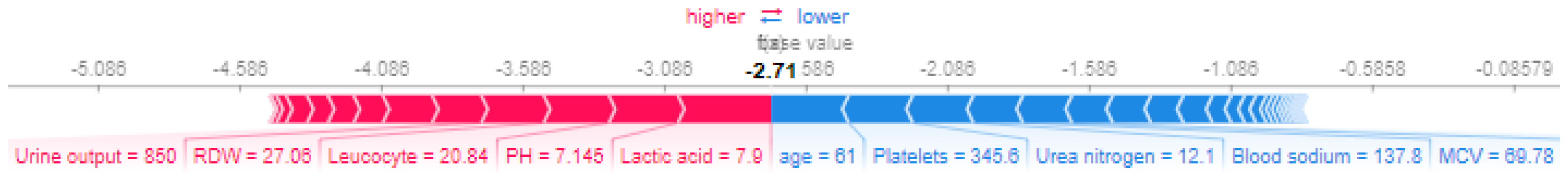
• The role of features in the prediction process was analyzed using SHAP in this study, providing insight into the determinant features that decide mortality in the ICU.

2. Background Studies

In this section, we review earlier research on nature-based feature selection in order to assess how well these algorithms handle feature selection challenges. In order to identify the research gaps, studies on mortality prediction that used scoring-based systems, ML, and deep learning were also evaluated.

2.1. Nature-Based Algorithms in Feature Selection Used in Different Studies

Many recent studies have started using nature-based algorithms in different areas for feature selection and to achieve higher accuracy. Some of these studies are included in this section.

In [5], for the feature selection problem, a new hybrid model based on the idea of opposition based learning (OBL) was provided that combines the whale optimization algorithm (WOA) and the FPA. The result obtained from experience showed that the proposed algorithm was more successful in terms of accuracy. The dataset used for this experiment is from the University of California Irvine (UCI) data repository and spam email dataset. In order to increase classification performance, the authors of [6] suggested combining the binary flower pollination algorithm (BFPA) and improved binary particle swarm optimization (iBPSO) with naive Bayes (NB) and K-nearest neighbor (K-NN). Results from the experiment show that the hybrid iBPSO BFPA outperformed the current strategy by achieving the highest accuracy of 94.43%. In [7], researchers presented an enhanced adaptive FPA that can alter its parameter settings dynamically during the convergence process and keep track of the optimum solution. The experimental findings showed that the other strategies with nine benchmark functions from the literature performed better, with a faster convergence rate. In order to reduce computational complexity, the authors of [18] proposed a wrapper–filter combination of ant colony optimization (ACO) to which they introduced subset evaluation using a filter approach rather than a wrapper method. Utilizing K-NN and multilayer perceptron classifiers, their suggested strategy was tested on several real-world datasets collected from the UCI ML repository and the NIPS2003 feature selection challenge. Comparison of the findings demonstrates unequivocally that their method outperforms the majority of the cutting-edge feature selection algorithms. To improve the accuracy of heart disease categorization, in [8], researchers used the fast correlation-based feature selection (FCBF) method to filter out redundant information. They then carried out classification using various classification algorithms, including K-NN, support vector machine (SVM), NB, RF, and a multilayer perception artificial neural network optimized by PSO combined with ACO approaches. Using the improved model suggested by FCBF, PSO, and ACO, the maximum classification accuracy was 99.65%. The purpose of [19] was to provide a thorough analysis of the nature-inspired metaheuristics used in the feature selection field. This review-based study discovered the answers to four research questions, including the number of metaheuristic techniques, their use, various feature selection methods, their contributions to the field of feature selection, and the frequency with which articles based on these techniques are published. To handle feature selection tasks, a novel gravitational search-approach-based algorithm with evolutionary crossover and mutation operators was proposed in [20]. K-NN and DT classifiers were both employed as evaluators for the proposed wrapper feature selection technique. A total of 18 well-known UCI datasets were used to evaluate the effectiveness of the suggested methods. The thorough results and comparisons show that the proposed model greatly outperforms previous wrapper approaches and has virtues in terms of exploration and exploitation, tradeoffs between searching trends, and faster convergence rates compared to other peers on a number of feature selection tasks. The authors of [21] used RF to choose the key characteristic for classification. Additionally, they assessed and contrasted each classification model’s accuracy and performance, including linear discriminant analysis (LDA), RF, SVM, and K-NN. The results of the experiments show that RF performed better across all experimental groups. According to another review [22], RF, SVM, LR, and k-NN are the ML algorithms most frequently employed for microbiome analysis. This review article provided an overview of the feature selection techniques used in ML applications for research on the human microbiome. Wrapper feature selection grey wolf optimization and PSO were combined with a new binary variation proposed in [23]. The best answers were discovered using the K-NN classifier with Euclidean separation matrices. Twenty datasets were used for the tests, and statistical analyses were conducted to evaluate the performance and efficacy of the suggested model using metrics including the ratio of selected features, classification precision, and computing time. In contrast to other algorithms’ accuracy levels of 81.6 and 86.8, the average accuracy was 90%. To address the issue of feature selection, the authors of [24] also proposed a brand-new, quick conditional mutual information feature selection algorithm. The experimental results demonstrate the viability of the suggested feature selection technique for constructing a high-level intelligent system to detect heart disease using a classifier SVM. In [25], binary variations of the recently developed grasshopper optimisation algorithm (GOA) were suggested and used to choose the best feature subset for classification in a wrapper-based framework. The comparative results demonstrate the improved performances of the binary GOA and binary GOA-M approaches when compared to similar techniques in the literature. The suggested binary GOA (specifically binary GOA-M) has strengths among the present feature selection algorithms and should be taken into consideration when tackling difficult feature selection problems according to the results, discussions, and assessments. The WOA, the artificial bee colony optimization (BCO) algorithm, and the PSO algorithm were the three algorithms that the authors of [9] identified as having the highest accuracy and having the potential to be used with their dataset to provide accurate diagnoses and potential treatments. The authors of [26] introduced the chaotic crow search algorithm (CCSA), a novel metaheuristic optimizer, to address the issues of low convergence rate and entrapment in local optima. According to experimental findings, CCSA can identify an ideal feature subset that maximizes classification performance while reducing the number of selected features. The experimental findings demonstrate that in terms of the best and mean fitness values, CCSA surpasses the other algorithms. The extended wrapper-based feature selection method described in [27] is based on a parallel novel intelligent GA. The outcomes show that the proposed model is capable of greatly generalizing the proposed multipopulation intelligent GA for datasets with two or more classes. By lowering the number of features from 56 to 28, 34 to 18, 279 to 135, 30 to 16, and 19 to 9 under lung cancer, dermatology, arrhythmia, and hepatitis, respectively, the researchers were able to achieve average classification accuracies of 95.83%, 97.62%, 99.02%, and 98.51%, respectively. In [28], researchers compared and analyzed several nature-inspired algorithms to choose the best traits and factors for distinguishing impacted patients from others. The experimental results demonstrate that the binary bat algorithm beat conventional methods, with a competitive recognition rate on the dataset of chosen features, including PSO, GA, and the modified cuckoo search algorithm.

2.2. Scoring-Based Mortality Prediction

Predictive scoring systems are disease severity measurements that are utilized to predict outcomes of a patient’s condition, most commonly mortality, in the ICU. Some common scoring systems for mortality forecasting include the Acute Physiology and Chronic Health Evaluation (APACHE) [29], the Sequential Organ Failure Assessment Score (SOFA) [30], and the Simplified Acute Physiology Score (SAPS) [31]. Aperstein et al. [32] developed a computational model that can predict mortality using a set of SOFA scores. When compared to previous years’ work, they discovered that an ensemble model of linear and LR yields a higher AUROC. Jentzer et al. [33] assessed the performance of the Acute Physiology and Chronic Health Evaluation (APACHE)-III, APACHE-IV, the Sequential Organ Failure Assessment (SOFA), and the Oxford Acute Severity of Illness Score (OASIS). In the CICU group, the assessed risk scores revealed uneven performance for mortality risk categorization across admission diagnoses. Traditional scoring methods, on the other hand, do not fully utilize a vast quantity of patient data and can only forecast with a limited degree of accuracy.

2.3. Machine-Learning-Based Mortality Prediction

Lin et al. [34] utilized the RF algorithm to develop a model for predicting mortality for acute renal patients in the ICU. They compared the model’s performance to that of the customized simplified acute physiology score (SAPS) II model and two other ML models. They discovered that in comparison to other models, theirs had the best accuracy and discrimination, as evaluated by Brier score and AUROC. Li et al. [35] are a group of researchers who proposed a novel approach using XGBoost and least absolute shrinkage and selection operator (LASSO) regression; the researchers were able to identify independent risk variables for in-hospital mortality in ICU-admitted heart failure patients. The calibration of the XGBoost and LASSO regression models was also quite good. According to this study, in a paired comparison, the XGBoost and LASSO regression models achieved better predicted performance than the Guidelines-Heart Failure (GWTG-HF) risk score model. Gu et al. [36] suggested a DELAK (dynamic ensembling learning algorithm based on k-means) to predict ICU mortality. In most mortality prediction tests, DELAK outperformed six other fusion processes; traditional scoring systems; classical ensemble models including AdaBoost, bagging, and RF; and dynamic ensemble selection approaches in terms of AUROC and Area under the rust progress curve (AURPC). Rashidy et al. [37] used different ML algorithms to present an ensemble strategy to predict ICU patient mortality. The study’s model exceeded state-of-the-art approaches in terms of accuracy according to the findings (94.4%). Ghorbani et al. [38] proposed a novel hybrid prediction model based on a combination of stacking and boosting ensemble methods and a new ensemble classifier based on the GA as a feature selection methodology. The suggested model was compared to the APACHE and SAPS scoring systems for experimental validation, and it outperformed the state-of-the-art models, yielding promising results. To effectively manage COVID-19 patients admitted to a medical unit, Allenbach et al. [39] developed a method to identify early prognostic indicators upon arrival. Using multivariable LR models, the predictors of ICU transfer or death on day 14, as well as being released alive or in a severe state on day 14 (remaining on ventilation or death), were investigated. Chiew et al. [40] compared the Combined Assessment of Risk Encountered in Surgery (CARES) model with the American Society of Anesthesiologists Physical Status (ASA-PS) in terms of predicting 30-day post-surgical mortality and the necessity for a more than 24 h ICU stay. With AUPRCs of 0.23 and 0.38 for mortality and ICU admission outcomes, respectively, GB was shown to be the best-performing model to develop forecasting models. Kong et al. [41] used the LASSO, RF, and gradient boosting machine (GBM) algorithms, as well as the standard LR method. In terms of prediction, the ML-based models developed in this study performed well. The GBM model performed the best in terms of forecasting the chance of in-hospital death according to this study. In a study of COVID-19 patients, Subudhi et al. [42] evaluated the effectiveness of 18 ML methods for forecasting ICU admission and death. Ensemble-based models outperformed other model types in predicting COVID-19 5-day ICU admission and 28-day mortality according to this study. Banoei et al. [43] developed an ML prediction model based on COVID-19 patient demographics, clinical factors, comorbidities, and biochemical markers. This model was able to predict COVID-19 hospital mortality with moderate predictive power, with Q2 equal 0.24 and high-accuracy AUROC greater than 0.85 by discriminating non-survivors from survivors using training and validation data. Raj et al. [44] utilized easy and widely scalable ML-based techniques to forecast mortality in real time during traumatic brain injury in critical care. Based on only three and four significant characteristics, their basic algorithms separated survivors from non-survivors with accuracies of up to 81 percent and 84 percent, respectively. The research works that have utilized different ML algorithms to predict the mortality rate in ICU are summarized in

Table 1. Summary of ML-based research works.

Ref.	Algorithm	Feature Selection	Interpretation	Dataset	Outcome
[34]	RF	No	No	MIMIC-III	Accuracy: 0.73
[35]	LR	XGBoosting	No	MIMIC-III	AUROC: 0.8416
[36]	Ensemble Method	No	No	MIMIC-III	AUROC: 83.91
[38]	Ensemble Method	GA	No	MIMIC-III	Accuracy: 82.5%
[41]	GBM	No	No	MIMIC-III	AUROC: 0.845

.

The analysis presented in this section reveals that numerous researchers have already employed various ML models to forecast ICU mortality. Two of the studies used feature selection in their research. No study used explainable AI to make the models transparent. Therefore, we believe that the field of ICU mortality prediction can be further enriched by comparing ML models with and without feature selection. As nature-based algorithms are successful in other fields, they can also be applied in this field in comparative studies.

2.4. Deep-Learning-Based Mortality Prediction

Deep-learning-based studies [45,46,47] in different areas becoming increasingly popular. Meyer et al. [46] created an explainable long short-term memory (LSTM) model to predict ICU mortality after 90 days. According to model interpretation, they discovered that input qualities might interact and compensate for one another, pulling towards survival in one direction and towards non-survival in the other direction. Using bidirectional LSTM, Yu et al. [47] developed a new paradigm for mortality prediction. They discovered that the deep-learning-based approach outperforms the existing SAPS-II severity assessment system. Bidirectional extended short-term memory outperformed the other methods, owing to its ability to capture both forward and backward temporal dependencies. Kim et al. [48] used deep learning to create a pediatric risk of mortality prediction tool. This study obtained an AUROC in the range of 0.89 to 0.97 for mortality prediction 6 to 60 h before death. By using LR and the extreme GB algorithm, the first in-hospital mortality prediction nomogram was developed. A deep multiscale convolutional neural network (CNN) architecture trained on the MIMIC-III dataset was proposed in [49] for mortality prediction. According to this study, the model has a AUROC of 0.8735 (0.0025), which is similar to the state of the art of deep learning mortality models trained on MIMIC-III data while still being interpretable. In the [5], in order to identify the most optimal lab events that contribute the most to mortality, an algorithm based on genetics and wrapper feature selection method was demonstrated. For experimental validation, the proposed model was compared to four popular traditional mortality assessments, as well as state-of-the-art ML models. In terms of the AUROC, the proposed model outperformed traditional scoring systems by 11–29% and state-of-the-art models by up to 14%. The authors of [50] used clinical data to construct a deep learning algorithm and a risk-score system for predicting ICU admission and in-hospital death in COVID-19 patients. The deep learning model predicted ICU admissions and mortality with AUROC values of 0.780 and 0.844, respectively. AUROCs of 0.728 and 0.848 were found for the associated risk ratings.

Research works that have utilized different ML algorithms to predict the mortality rate in the ICU are summarized below in

Table 2. Summary of deep-learning-based research works.

Ref.	Algorithm	Feature Selection	Interpretation	Dataset	Outcome
[46]	LSTM	No	Yes	Collected	AUROC: 0.88
[47]	LSTM	No	No	MIMIC-III	AUROC: 0.8854
[49]	CNN	No	Yes	MIMIC-III	AUROC: 0.8735
[50]	Deep Learning	No	No	Collected	AUROC: 0.84

.

The analysis presented in this section shows that deep learning with interpretation has been utilized in related studies. Feature selection was proposed as a potential improvement in [49]. Therefore, we believe that this area of ICU mortality prediction can be expanded and enhanced.

3. Materials and Methods

3.1. Workflow Diagram

Figure 1 shows the workflow diagram of this research. As previously indicated, the dataset used for this study was obtained from the popular MIMIC-III data repository, which is depicted in the first stage of the workflow diagram. However, because the dataset contained null values, it was necessary to preprocess the data by filling in the blank values.

Subsequently, feature selection was carried out. Three feature selection algorithms, namely FPA, PSO, and GA, were used to select features. The selected features were then subjected to ML models. We also observed how the ML models functioned without feature selection. Accuracy and the AUROC curve were used to assess performance. Finally, SHAP was used to observe the decision-making process of the ML models.

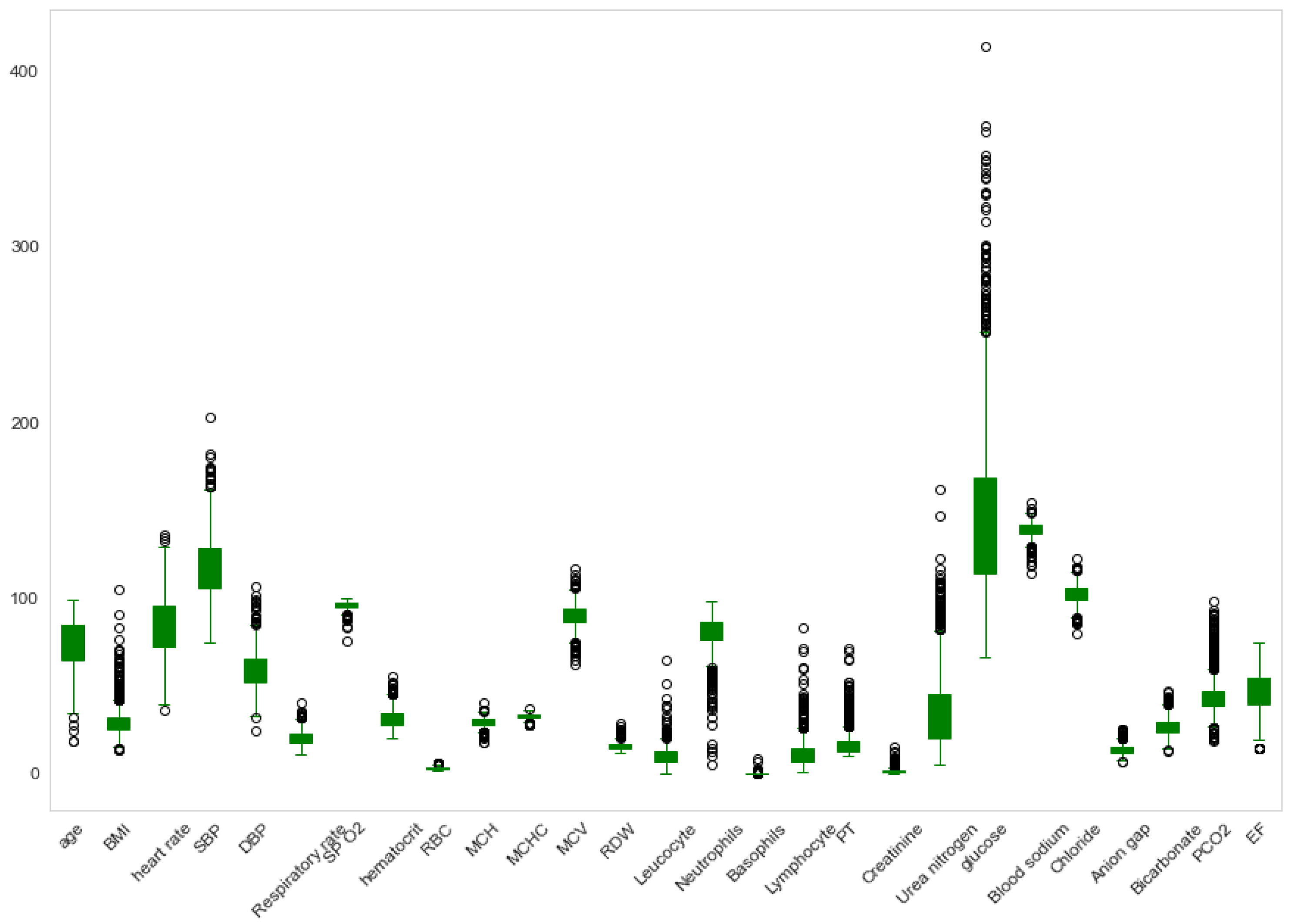
3.2. Dataset Description

A total of 1177 cases were included in the dataset utilized in this study for in-hospital mortality prediction, with a total of 51 features. Here, the desired value of ‘0’ denotes life, and ‘1’ denotes death. Age, gender, and BMI were the demographic factors studied. The vital signs were heart rate, blood temperature, blood pressure, respiratory rate, saturation pulse oxygen, and urine output. Comorbidity characteristics include hypertension, atrial fibrillation, diabetes, depression, and hyperlipidemia. Red blood cells, white blood cells, neutrophils, basophils, lymphocytes, potassium, sodium, anion gap, lactate, bicarbonate, calcium, chloride, magnesium, creatinine, creatine kinase, and prothrombin time, are some of the laboratory variables. A statistical analysis of the dataset features is shown in

Table 3. Statistical Analysis of dataset features.

Feature	Mean	Standard Deviation	Min	25%	50%	75%	Max
Age	74.05	13.43	19.00	65.00	77.00	85.00	99.00
BMI	30.19	9.33	13.35	24.33	28.31	33.63	104.97
Hypertensive	0.72	0.45	0.00	0.00	1.00	1.00	1.00
Atrial fibrillation	0.45	0.49	0.00	0.00	0.00	1.00	1.00
CHD with no MI	0.09	0.28	0.00	0.00	0.00	0.00	1.00
Diabetes	0.42	0.49	0.00	0.00	0.00	1.00	1.00
Deficiency anemias	0.34	0.47	0.00	0.00	0.00	1.00	1.00
Depression	0.12	0.32	0.00	0.00	0.00	0.00	1.00
Hyperlipidemia	0.38	0.48	0.00	0.00	0.00	1.00	1.00
Renal failure	0.37	0.48	0.00	0.00	0.00	1.00	1.00
COPD	0.08	0.26	0.00	0.00	0.00	0.00	1.00
Heart rate	84.58	16.01	36.00	72.37	83.61	95.90	135.70
Systolic BP	118.00	17.37	75.00	105.38	116.15	128.63	203.00
Diastolic BP	1161.00	10.68	24.73	52.17	58.46	65.46	107.00
Respiratory rate	1164.00	4.00	11.13	17.92	20.37	23.39	40.90
Temperature	1158.00	0.60	33.25	36.28	36.65	37.02	39.13
SP O2	1164.00	2.29	75.91	95.00	96.45	97.91	100.00
Urine output	1899.28	1272.36	0.00	980.00	1675.00	2500.00	8820.00
Hematocrit	31.91	5.20	20.31	28.16	30.80	35.01	55.42
RBC	3.57	0.62	2.03	3.12	3.49	3.90	6.57
MCH	29.54	2.61	18.12	28.25	29.75	31.24	40.31
MCHC	32.86	1.40	27.82	32.01	32.98	33.82	37.01
MCV	89.90	6.53	62.60	86.25	90.00	93.85	116.71
RDW	15.95	2.13	12.08	14.46	15.51	16.93	29.05
Leucocyte	10.71	5.22	0.10	7.44	9.68	12.74	64.75
Platelets	241.50	113.12	9.57	168.90	222.66	304.25	1028.20
Neutrophils	80.11	11.13	5.00	74.77	82.46	87.45	98.00
Basophils	0.41	0.46	0.10	0.20	0.30	0.50	8.80
Lymphocyte	12.23	8.63	0.96	6.65	10.47	15.46	83.50
PT	17.48	7.38	10.10	13.16	14.63	18.80	71.27
INR	1.62	0.83	0.87	1.14	1.30	1.73	8.34
NT-proBNP	11,014.13	13,148.66	50.00	2251.00	5840.00	14,968.00	118,928.00
Creatine kinase	246.77	1484.52	8.00	46.00	89.25	185.18	42,987.50
Creatinine	1.64	1.27	0.26	0.94	1.28	1.90	15.53
Urea nitrogen	36.29	21.85	5.35	20.83	30.66	45.25	161.75
Glucose	148.79	51.49	66.66	113.93	136.40	169.50	414.10
Blood potassium	4.17	0.41	3.00	3.90	4.11	4.40	6.56
Blood sodium	138.89	4.15	114.66	136.66	139.25	141.60	154.73
Blood calcium	8.50	0.57	6.70	8.14	8.50	8.86	10.95
Chloride	102.28	5.34	80.26	99.00	102.50	105.57	122.52
Anion gap	13.92	2.65	6.63	12.25	13.66	15.41	25.50
Magnesium ion	2.12	0.25	1.40	1.95	2.09	2.24	4.07
PH	7.37	0.06	7.09	7.33	7.38	7.43	7.58
Bicarbonate	26.91	5.16	12.85	23.45	26.50	29.87	47.66
Lactic acid	1.85	0.98	0.50	1.20	1.60	2.20	8.33
PCO2	45.53	12.71	18.75	37.04	43.00	50.58	98.60
EH	48.71	12.86	15.00	40.00	55.00	55.00	75.0

.

3.3. Data Preprocessing

We investigated whether the dataset contained any null values prior to the preprocessing stage. In order to determine whether any of the data points were outliers, box plots for the features were also analyzed. Some of the features, namely hypertensive, atrial fibrillation, CHD with no MI, diabetes, deficiency anemias, depression, hyperlipidemia, renal failure, and COPD, had values of 0 and 1, which is why box plots were not generated for those features. The box plots for the rest of the features are shown in Figure 2.

The features with no outliers were removed from Figure 2. Features with outliers were removed in the preprocessing step. Furthermore, null values were imputed, and superfluous columns were removed in this step. In the columns of dependent variables such as BMI, heart rate, systolic blood pressure, diastolic blood pressure, respiratory rate, temperature, urine output, neutrophils, basophils, glucose, blood calcium, creatine kinase, and lactic acid, there were numerous null values. There was also an independent null value in the “Output” field. As a result, the dependent null values of float and integer types were imputed with the mean value of the respective column. Furthermore, the null value in the independent column “outcome” was imputed with the most frequent value of the column. The ID field was removed from the dataset because it has no bearing on the prediction. We also found that the dataset was imbalanced. A total of 1017 records were found for output ‘0’ or alive, and 159 records were found for class ‘1’ or death. The synthetic minority oversampling technique (SMOTE) was used in this study to handle the imbalanced data. SMOTE is a statistical technique for increasing the number of cases in a dataset in a balanced manner. The component creates new instances from existing minority cases.

3.4. Feature Selection Algorithm

The aim of feature selection is to reduce the number of predictors while training an ML model to speed up computations and enhance prediction accuracy. The filter method, wrapper method, and embedding method are the three primary divisions of the feature selection procedure. The nature-based feature selection methods used in this study follow the wrapper feature selection method. Therefore, before going into the details of these feature selection methods, a brief summary of the wrapper feature selection method is presented below.

3.4.1. Wrapper Feature Selection Method

Wrapper approaches compare the performance of several models by adding or removing variables. These processes are typically developed using the idea of the greedy search algorithm. In this method, a subset of features is first selected from the whole feature; then the feature set is applied to an ML algorithm. Lastly, the performance of that model is measured. This process is repeated until an optimal feature set is found. The flow chart for the wrapper selection process is shown in Figure 3.

Forward selection, backward elimination, and bidirectional elimination are the most used techniques under wrapper feature selection. The forward selection procedure begins with one predictor and gradually adds more. In the backward elimination process, the process starts with all predictors, which are then iteratively eliminated one by one. The bidirectional elimination process is the combination of forward selection and backward elimination.

For feature selection, three nature-based algorithms, namely the FPA, GA, and PSO, were utilized. The following are the working mechanisms of these feature selection algorithms.

3.4.2. Flower Pollination Algorithm

This FPA [10] is a nature-based, population-based optimization technique that mimics how flowering plants pollinate one another. The pollination process can be divided into two types:

Local Pollination/Self Pollination/Abiotic PollinationThis type of pollination occurs within a flower itself or within two different flowers of the same tree. There is no need for pollinators in this process. Global Pollination/Cross Pollination/Biotic Pollination: In this process, pollination occurs by transferring pollen from one flower to another flower of two different trees. Pollinators are needed in this pollination process.

The initial population size, switch probability, and a maximum number of generations are set for this method at the beginning. In the following phase, the fitness function for each population solution is assessed by computing the corresponding objective function. In the next step, either local pollination or global pollination is evaluated until termination criteria are satisfied. Then, each solution is reviewed and updated according to the objective values. Finally, ranking of the solutions reveals the best one.

3.4.3. Genetic Algorithm

The GA [12], a technique for the optimization problem, was influenced by Charles Darwin’s notion of natural evolution. The fittest individuals are picked for reproduction in order to give rise to the next generation’s offspring, which is how natural selection works. The initial population, fitness function, selection, crossover, and mutation are the five most important phases of the GA.

This algorithm’s initial step is to generate a population or initial generation of potential answers to the problem at random. The fitness function gauges an individual’s fitness level. Each individual receives a fitness rating from the system. In the selection phase, the fittest individuals are selected for further steps. The crucial stage of the GA is crossover. A crossover point is picked randomly from the DNA for each set of parents to mate. Parents’ genes are exchanged among one another until the crossover point is achieved, at which point offspring are produced. To put it simply, a mutation is a minor, haphazard change made to a chromosome in order to produce a new outcome. It serves to preserve and increase genetic population diversity. The algorithm typically comes to an end when the population has reached a desirable level of fitness or the maximum number of generations has been produced.

3.4.4. Particle Swarm Algorithm

As a bio-inspired algorithm, the PSO [11] is straightforward in its search for the best solution in the problem area. It is a stochastic optimization technique that is based on how swarms move and function. Two of the most important concepts in this algorithm are the scores of personal best and global best. Personal best is the best result of any single particle, and global best is the best value of any particle in the swarm.

In this algorithm, first, a population of particles is initialized. Then, the fitness value is calculated for each particle. If the fitness value is better than the personal best, the current value is set as the personal best. Then, the particle with the best fitness value of all particles is found. Lastly, the velocity and position of a particle are updated. This process continues until max iteration or min error criteria are attained.

3.5. Machine Learning Algorithm

Four ML algorithms, namely LR, DT, RF, and GB, were utilized in this study. The following are the working mechanism of these classifiers.

3.5.1. Logistic Regression Algorithm

LR [13] is a supervised machine learning algorithm used to solve classification problems based on the concept of probability. It can be used while the dependent variable is categorical. The aim of this algorithm is to determine the best-fitting model to interpret the relationship between the independent and dependent variables. This algorithm is categorized into binary, multinomial, ordinal, etc., categories.

To map the predicted values to probabilities, the sigmoid function is used by this algorithm, which maps any real value between 0 and 1. The sigmoid function is expressed by Equation (1) [51].

$$f\left(x\right)=1/(1+e^{-z})$$

(1)

In Equation (1), if the value of z increases to a positive infinity, the anticipated value of f(x) is 1, and if it decreases to a negative infinity, f(x) is 0. The threshold value is a notion used in LR. The threshold values aid in determining whether there is a chance of 0 or 1. For instance, a value below the threshold value tends to be 0, whereas a value over the threshold value tends to be 1. Cross entropy, commonly known as log loss and the difference between the actual and predicted value, is the cost function used in this algorithm. Gradient descent, which calculates the model’s parameters or weights, is used to reduce costs. Thus, the prediction process is done in LR.

3.5.2. Decision Tree Algorithm

A DT [16] algorithm is a supervised ML algorithm that can be used to solve both classification and regression problems. The term itself implies that it displays the predictions that come from a sequence of feature-based splits using a flow chart that resembles a tree structure. The decision is made by the leaves at the end, which follow the root node. Finding the attribute for the root node at each level of the DT presents a significant difficulty. The Gini index and information gain are two common methods of attribute selection in the DT algorithm.

Information Gain: The reduction in uncertainty for a given feature is measured by information gain, which also determines which attribute should be chosen as a decision node or root node.

Gini Index: The Gini Index is a potent indicator of the randomness, impurity, or entropy of a dataset’s values. The aim of the Gini index of a DT model is to reduce impurities from the root nodes to the leaf nodes, which implies that a lower Gini index for an attribute should be chosen. The Gini index is determined by deducting the sum of the squared probabilities of each class from one.

3.5.3. Random Forest Algorithm

A supervised ML technique known as the RF [15] or random decision forest algorithm is used for classification, regression, and other tasks using decision trees. A randomly chosen portion of the training data is used by the RF classifier to generate a collection of decision trees. It simply consists of a collection of decision trees from a randomly chosen subset of the training set, which is subsequently used to decide the final prediction. The total process is shown in Figure 4. Here, the training dataset is divided into subsets, and from every subset of training data, a DT is made. Finally, by averaging the prediction from every DT, the final decision is made.

This technique is also called an ensemble technique, as it combines multiple models. The RF algorithm attempts to produce an uncorrelated forest of trees whose forecast by committee is more accurate than that of any individual tree by using bagging and feature randomness when generating each individual tree.

3.5.4. Gradient Boosting Algorithm

GB [14] is a type of boosting strategy that builds a strong model by iteratively learning from each of the weak learners. It can be used to solve both classification and regression problems. A GB classifier has three main components, namely a loss function, a weak learner, and an additive model. The purpose of the loss function is to calculate how well the model predicts, given the available data. A weak learner attempts to categorize data but performs poorly, possibly no better than guessing at random. This method adds weak learners one step at a time in an iterative and sequential manner, gradually approaching the final model with each cycle. In other words, the value of the loss function should decrease with each repetition.

4. Result Analysis

4.1. Comparison of Performance

The performances of four ML models were examined in this experiment. Three nature-based algorithms—FPA, PSO, and GA—were employed for feature selection. Performance was measured in terms of accuracy. The accuracy score was determined by dividing the number of accurate forecasts by the total number of predictions.

In this study, a fivefold cross-validation process was used for training and testing. The final accuracy was determined by averaging the accuracy results from each fold. Results of the experiment with and without feature selection are displayed in

Table 4. Comparison of the performance (accuracy) of different ML Models with and without feature selection.

Model Name	No Feature Selection	With Feature Selection
		FPA	PSO	GA
LR	69.9%	71.6%	57.3%	69.0%
DT	82.50%	84.8%	81.8%	75.1%
RF	90.9%	92.8%	90.6%	92.4%
GB	91.0%	91.1%	83.9%	81.3%

:

Table 4 shows that accuracy of the ML models is relatively high when features are selected with the FPA. Therefore, this feature selection process can help physicians to make decisions while considering fewer features.

Table 5. Features selected by different algorithms.

Algorithm	Number of Selected Features	Feature Names
FPA	21	Age, BMI, hypertensive, atrial fibrillation, depression, Renal failure, COPD, heart rate, SP O2, hematocrit, RBC, MCV, MCHC, platelets, blood sodium, creatine kinase, creatinine, urea nitrogen, blood calcium, chloride, and magnesium ion
PSO	17	Hypertensive, atrial fibrillation, depression, COPD, heart rate, systolic blood pressure, temperature, hematocrit, MCH, RDW, lymphocyte, urea nitrogen, anion gap, PH, bicarbonate, lactic acid, and PCO2
GA	12	Age, BMI, systolic blood pressure, diastolic blood pressure, respiratory rate, hematocrit, MCH, MCHC, neutrophils, PT, blood sodium, and lactic acid.

shows the features selected by different nature-based algorithms.

Because the FPA outperformed all others method in this study in terms of accuracy, the features chosen by this algorithm can be considered important. Common features selected by at least two of the nature-based algorithms are age, BMI, hypertensive, atrial fibrillation, depression, COPD, heart rate, hematocrit, Blood Sodium, Urea nitrogen, systolic blood pressure, MCH, MCHC, and lactic acid.

4.2. AUROC Curve Analysis

The true-positive and false-positive rates were plotted against each other at different threshold settings on an AUROC probability curve, revealing how well the model differs across classes. The model is more accurate in classifying 0 classes as 0 and classifying 1 classes as 1 with higher AUROC values.

The AUROC curves for ML models without feature selection and with feature selection via FPA, PSO, and GA are shown in Figure 5.

According to the results, ML models using the FPA feature selection algorithm also perform well in terms of AUROC values.

4.3. Statistical Test Results

To solve the problem of selecting the best model, statistical significance tests were used. The Friedman test was used in this study to compare machine learning classifiers. The Friedman test results are shown in

Table 6. Friedman test results.

Friedman Test	Degrees of Freedom	Chi-Square	p-Value
	3	11.1	0.0112

and

Table 7. Additional information from Friedman test results.

Rank	Feature Selection with the Classifiers	Rank Sum
1	FPA	16
2	No feature selection	11
3	GA	7
4	PSO	6

. These result indicate that the p-value is 0.0112. The null hypothesis is rejected because the p-value for classifier accuracy data is less than the significance level of 0.05, indicating that the classifiers perform differently.

4.4. Proposed Model vs. Literature Studies

In this section, we present a comparison between our suggested model and models proposed in the literature in terms of accuracy, AUROC score, and the number of features. It should be noted that different MIMIC-III datasets were used in the several studies described here. However, all of the studies analyzed here were conducted for the purpose of mortality prediction in the ICU. The AUROC scores of our model and those proposed in other studies are presented in

Table 8. Comparison of performance ( AUROC) of different ML models proposed in the literature.

Study	Year	Dataset	Sample	Algorithm	Number of Features	AUROC Score
[52]	2021	MIMIC-III	25,659	XGBoost	66	82%
[53]	2022	MIMIC-III	6699	Ensemble	20	82.55%
[36]	2021	MIMIC-III	58,976	Dynamic Ensemble	28	83.91%
[41]	2020	MIMIC-III	16,688	GB	86	84%
RF + PSO	2023	MIMIC-III	1177	RF + FPA	21	83.0%

. The RF model utilized in this study with the FPA feature selection algorithm achieved an 83.0% AUROC score with only 21 features. Our proposed model is compared with those proposed in other studies in literature in term of accuracy in

Table 9. Comparison of the performance (accuracy) of different ML models proposed in the literature.

Study	Year	Dataset	Sample	Algorithm	Number of Features	Accuracy
[54]	2019	MIMIC-III	5037	Logistic Model Trees	79	85.12%
[35]	2021	MIMIC-III	1177	XGBoost	20	76%
[34]	2019	MIMIC-III	19,044	RF	15	72.8%
LR + FPA	2023	MIMIC-III	1177	RF + FPA	21	92.80%

. The RF algorithm with FPA feature selection achieved the highest accuracy of 92.80% with only 21 features.

5. Interpretation of Results with SHAP

A game theoretic technique called SHAP can be used to explain the output of any ML model. Estimating the contribution of each feature in a dataset to the prediction made by the model is possible with feature importance. It is possible to determine which features have the greatest influence on a model’s decision making by executing feature importance tests. This allows us to eliminate features that have little bearing on the model’s predictions and concentrate on enhancing the more important features.

In this research, SHAP was used to explain the model both globally and locally. Figure 6 shows the 20 most important features that influence the prediction process. This list shows the most important features in descending order. The SHAP value is shown on the x-axis of the graph, while all the features are shown on the y-axis. One SHAP value for a prediction and a feature is represented by each point on the graph. Red indicates higher feature values, whereas blue denotes lower feature values. The directionality influence of the characteristics can be generalized based on the distribution of the red and blue dots.

The features selected by SHAP matched the features selected by the FPA. Eleven features were common in both of the processes. The common features selected by the FPA and SHAP are blood sodium, heart rate, age, blood calcium, renal failure, platelets, urea nitrogen, MCV, creatinine, chloride, and BMI. Figure 6 shows that higher lymphocyte values increase the likelihood of survival, while lower lymphocyte values increase the chance of mortality. Higher age values lead to death, whereas lower age values lead to survival. The impact of other features on the prediction can be analyzed in the same manner.

The local interpretability of SHAP made the ML models more transparent by explaining why a case receives its prediction and the contributions of the features to the forecast. Below, we analyze some instances using SHAP to observe the prediction process of the ML model. Features that make a prediction of a positive outcome or death more likely are displayed in red, while those that make a prediction of a negative outcome or survival more likely are displayed in blue.

In interpretation 1 shown in Figure 7, the features that were crucial to predicting an instance are depicted in red and blue, with red denoting features that increased the model score and blue denoting features that decreased the score. The closer the feature is to the line separating red from blue, the more of an impact it had on the score, and the size of the bars indicates the extent of the impact. The features blood sodium, RDW, and chloride push the predictions toward a positive outcome, whereas deficiency anemias, age, platelet, heart rate, renal failure, BMI, and blood calcium push the predictions toward a negative outcome. Here, the real prediction made by the model is negative.

In interpretation 2 shown in Figure 8, the features deficiency anemias, lactic acid, chloride, blood calcium, and PH push the prediction to a positive outcome, whereas heart rate, and blood sodium push the outcome toward a negative outcome. Here, the real prediction made by the model is positive.

In interpretation 3 shown in Figure 9, the features of urine output, RDW, leukocyte, PH, and lactic acid push the prediction toward a positive outcome, whereas age, platelets, urine nitrogen, blood sodium, and MCV push the prediction toward a negative outcome. Here, the real prediction made by the model is negative.

In these three cases, the ML model makes predictions based on the most important selected features. Therefore, the less important features can be removed to increase the speed and ease of the prediction process. This process can be helpful for physicians to make a decision considering fewer features.

6. Conclusions

The aim of this research was to compare the performance of prediction models with and without feature selection using a nature-based algorithm for mortality prediction in the ICU for heart failure patients. We found that FPA, a nature-based feature selection algorithm, had a considerable impact on the performance of the ML models. With only 21 features selected by the FPA, the RF model showed the highest accuracy of 92.8%, as well as the highest AUROC value of 83.0%. When the performance of the model proposed in this study was compared to that of models proposed in the literature, we discovered that models with fewer features chosen by the FPA achieve the best performance. The model’s decision-making process was also explained by SHAP. We found that the features selected by SHAP and the FPA were the most common. We hope that this prediction model can assist physicians in the decision-making process by considering fewer features for the optimal use of ICU resources.

References

1. Al Mamun, S.; Kaiser, M.S.; Mahmud, M. An Artificial Intelligence Based Approach towards Inclusive Healthcare Provisioning in Society 5.0: A Perspective on Brain Disorder. In Proceedings of the Brain Informatics: 14th International Conference, BI 2021, Virtual Event, 17–19 September 2021; Springer International Publishing: Cham, Switzerland, 2021. Available online: https://link.springer.com/chapter/10.1007/978-3-030-86993-9 (accessed on 12 February 2023).
2. Heart Failure Projected to Increase Dramatically, According to New Statistics. 2021. Available online: https://www.heart.org/en/news/2018/05/01/heart-failure-projected-to-increase-dramatically-according-to-new-statistics (accessed on 23 November 2022).
3. Safavi, K.C.; Dharmarajan, K.; Kim, N.; Strait, K.M.; Li, S.-X.; Chen, S.I.; Lagu, T.; Krumholz, H.M. Variation exists in rates of admission to intensive care units for heart failure patients across hospitals in the United States. Circulation 2013, 127, 923–929. [Google Scholar] [CrossRef] [PubMed]
4. Johnson, A.; Pollard, T.; Mark, R. Mimic-III Clinical Database, MIMIC-III Clinical Database v1.4. 2016. Available online: https://physionet.org/content/mimiciii/1.4/ (accessed on 23 November 2022).
5. Mohammadzadeh, H.; Gharehchopogh, F.S. A Novel Hybrid Whale Optimization Algorithm with Flower Pollination Algorithm for Feature Selection: Case Study Email Spam Detection. Comput. Intell. 2021, 37, 176–209. [Google Scholar] [CrossRef]
6. Rajamohana, S.; Umamaheswari, K. A Hybrid Approach to Optimize Feature Selection Process Using IBPSO- BFPA for Review Spam Detection. Appl. Math. Inf. Sci. 2017, 11, 1443–1449. [Google Scholar] [CrossRef]
7. Rodrigues, D.; de Rosa, G.H.; Passos, L.A.; Papa, J.P. Adaptive Improved Flower Pollination Algorithm for Global Optimization. In Nature-Inspired Computation in Data Mining and Machine Learning; Yang, X.-S., He, X.-S., Eds.; Springer International Publishing: Berlin/Heidelberg, Germany, 2020; Volume 855, pp. 1–21. [Google Scholar] [CrossRef]
8. Khourdifi, Y.; Bahaj, M. Heart Disease Prediction and Classification Using Machine Learning Algorithms Optimized by Particle Swarm Optimization and Ant Colony Optimization. Int. J. Intell. Eng. Syst. 2019, 12, 242–252. [Google Scholar] [CrossRef]
9. Guha, J.; Chouksey, A.; Khodwe, P.; Inje, B.V. Review Paper of Nature-Based Optimization Algorithms for Medicine Predictor. Int. J. Eng. Res. Technol. 2021, 10, 179–185. [Google Scholar]
10. Yang, X.-S. Flower Pollination Algorithm for Global Optimization. In Unconventional Computation and Natural Computation; Durand-Lose, J., Jonoska, N., Eds.; Springer: Berlin/Heidelberg, Germany, 2012; pp. 240–249. [Google Scholar] [CrossRef]
11. Eberhart, R.; Kennedy, J. A new optimizer using particle swarm theory. In Proceedings of the Sixth International Symposium on Micro Machine and Human Science, Nagoya, Japan, 4–6 October 1995; pp. 39–43. [Google Scholar]
12. Holland, J.H. Adaptation in Natural and Artificial Systems, 2nd ed.; University of Michigan Press: Ann Arbor, MI, USA, 1992. [Google Scholar]
13. Menard, S. Applied Logistic Regression Analysis; No. 106; SAGE: Newbury Park, CA, USA, 2002. [Google Scholar]
14. Gradient Boosting. Wikipedia. Wikimedia Foundation. 2022. Available online: https://en.wikipedia.org/wiki/Gradient-boosting (accessed on 24 January 2023).
15. Random Forest. Wikipedia. Wikimedia Foundation. 2023. Available online: https://en.wikipedia.org/wiki/Random-forest (accessed on 24 January 2023).
16. Decision Tree. Wikipedia. Wikimedia Foundation. 2022. Available online: https://en.wikipedia.org/wiki/Decision-tree (accessed on 24 January 2023).
17. Linardatos, P.; Papastefanopoulos, V.; Kotsianti, S. Explainable AI: A Review of Macine Learning Interpretability Methods. Entropy 2021, 23, 18. [Google Scholar] [CrossRef]
18. Ghosh, M.; Guha, R.; Sarkar, R.; Abraham, A. A Wrapper-Filter Feature Selection Technique Based on Ant Colony Optimization. Neural Comput. Appl. 2020, 32, 7839–7857. [Google Scholar] [CrossRef]
19. Sharma, M.; Kaur, P. A Comprehensive Analysis of Nature-Inspired Meta-Heuristic Techniques for Feature Selection Problem. Arch. Comput. Methods Eng. 2021, 28, 1103–1127. [Google Scholar] [CrossRef]
20. Taradeh, M.; Mafarja, M.; Heidari, A.A.; Faris, H.; Aljarah, I.; Mirjalili, S.; Fujita, H. An Evolutionary Gravitational Search-Based Feature Selection. Inf. Sci. 2019, 497, 219–239. [Google Scholar] [CrossRef]
21. Chen, R.-C.; Dewi, C.; Huang, S.-W.; Caraka, R.E. Selecting Critical Features for Data Classification Based on Machine Learning Methods. J. Big Data 2020, 7, 52. [Google Scholar] [CrossRef]
22. Marcos-Zambrano, L.J.; Karaduzovic-Hadziabdic, K.; Loncar Turukalo, T.; Przymus, P.; Trajkovik, V.; Aasmets, O.; Berland, M.; Gruca, A.; Hasic, J.; Hron, K.; et al. Applications of Machine Learning in Human Microbiome Studies: A Review on Feature Selection, Biomarker Identification, Disease Prediction and Treatment. Front. Microbiol. 2021, 12, 313. [Google Scholar] [CrossRef] [PubMed]
23. El-Hasnony, I.M.; Barakat, S.I.; Elhoseny, M.; Mostafa, R.R. Improved feature selection model for big data analytics. IEEE Access 2020, 8, 66989–67004. [Google Scholar] [CrossRef]
24. Li, J.P.; Haq, A.; Swati, S.; Khan, J.; If, A.; Saboor, A. Heart Disease Identification Method Using Machine Learning Classification in E-Healthcare. IEEE Access 2020, 8, 107562–107582. [Google Scholar] [CrossRef]
25. Mafarja, M.; Aljarah, I.; Faris, H.; Hammouri, A.I.; Al-Zoubi, A.M.; Mir-Jalili, S. Binary Grasshopper Optimisation Algorithm Approaches for Feature Selection Problems. Expert Syst. Appl. 2019, 117, 267–286. [Google Scholar] [CrossRef]
26. Sayed, G.I.; Hassanien, A.E.; Azar, A.T. Feature Selection via a Novel Chaotic Crow Search Algorithm. Neural Comput. Appl. 2019, 31, 171–188. [Google Scholar] [CrossRef]
27. Sahebi, G.; Movahedi, P.; Ebrahimi, M.; Pahikkala, T.; Plosila, J.; Tenhunen, H. GeFeS: A Generalized Wrapper Feature Selection Approach for Optimizing Classification Performance. Comput. Biol. Med. 2020, 125, 103974. [Google Scholar] [CrossRef]
28. Shrivastava, P.; Shukla, A.; Vepakomma, P.; Bhansali, N.; Verma, K. A Survey of Nature-Inspired Algorithms for Feature Selection to Identify Parkinson’s Disease. Comput. Methods Programs Biomed. 2017, 139, 171–179. [Google Scholar] [CrossRef]
29. Knaus, W.A.; Draper, E.A.; Wagner, D.P.; Zimmerman, J.E. APACHE II: A Severity of Disease Classification System. Crit. Care Med. 1985, 13, 818. [Google Scholar] [CrossRef]
30. Vincent, J.L.; Moreno, R.; Takala, J.; Willatts, S.; De Mendonça, A.; Bruining, H.; Reinhart, C.K.; Suter, P.M.; Thijs, L.G. The SOFA (Sepsis-Related Organ Failure Assessment) Score to Describe Organ Dysfunction/Failure. On Behalf of the Working Group on Sepsis-Related Problems of the European Society of Intensive Care Medicine. Intensive Care Med. 1996, 22, 707–710. [Google Scholar] [CrossRef]
31. Le Gall, J.-R. A New Simplified Acute Physiology Score (SAPS II) Based on a European/North American Multicenter Study. JAMA J. Am. Med. Assoc. 1993, 270, 2957. [Google Scholar] [CrossRef]
32. Aperstein, Y.; Cohen, L.; Bendavid, I.; Cohen, J.; Grozovsky, E.; Rotem, T.; Singer, P. Improved ICU Mortality Prediction Based on SOFA Scores and Gastrointestinal Parameters. PLoS ONE 2019, 14, e0222599. [Google Scholar] [CrossRef] [PubMed]
33. Jentzer, J.C.; Diepen, S.; Murphree, D.; Ismail, A.; Keegan, M.; Morrow, D.; Barsness, G.; Anaveka, N. Admission Diagnosis and Mortality Risk Prediction in a Contemporary Cardiac Intensive Care Unit Population. Am. Heart J. 2020, 224, 57–64. [Google Scholar] [CrossRef] [PubMed]
34. Lin, K.; Hu, Y.; Kong, G. Predicting In-Hospital Mortality of Patients with Acute Kidney Injury in the ICU Using Random Forest Model. Int. J. Med. Inform. 2019, 125, 55–61. [Google Scholar] [CrossRef] [PubMed]
35. Li, F.; Xin, H.; Zhang, J.; Fu, M.; Zhou, J.; Lian, Z. Prediction Model of In-Hospital Mortality in Intensive Care Unit Patients with Heart Failure: Machine Learning-Based, Retrospective Analysis of the MIMIC-III Database. BMJ Open 2021, 11, e044779. [Google Scholar] [CrossRef]
36. Guo, C.; Liu, M.; Lu, M. A Dynamic Ensemble Learning Algorithm Based on K-Means for ICU Mortality Prediction. Appl. Soft Comput. 2021, 103, 107166. [Google Scholar] [CrossRef]
37. El-Rashidy, N.; El-Sappagh, S.; Abuhmed, T.; Abdelrazek, S.; El-Bakry, H.M. Intensive Care Unit Mortality Prediction: An Improved Patient-Specific Stacking Ensemble Model. IEEE Access 2020, 8, 133541–133564. [Google Scholar] [CrossRef]
38. Ghorbani, R.; Ghousi, R.; Makui, A.; Atashi, A. A New Hybrid Predictive Model to Predict the Early Mortality Risk in Intensive Care Units on a Highly Imbalanced Dataset. IEEE Access 2020, 8, 141066–141079. [Google Scholar] [CrossRef]
39. Allenbach, Y.; Saadoun, D.; Maalouf, G.; Vieira, M.; Hellio, A.; Boddaert, J.; Gros, H.; Salem, J.E.; Resche Rigon, M.; Menyssa, C.; et al. Development of a Multivariate Prediction Model of Intensive Care Unit Transfer or Death: A French Prospective Cohort Study of Hospitalized COVID-19 Patients. PLoS ONE 2020, 15, e0240711. [Google Scholar] [CrossRef]
40. Chiew, C.J.; Liu, N.; Wong, T.H.; Sim, Y.E.; Abdullah, H.R. Utilizing Machine Learning Methods for Preoperative Prediction of Postsurgical Mortality and Intensive Care Unit Admission. Ann. Surg. 2020, 272, 1133–1139. [Google Scholar] [CrossRef]
41. Kong, G.; Lin, K.; Hu, Y. Using Machine Learning Methods to Predict In-Hospital Mortality of Sepsis Patients in the ICU. BMC Med. Inform. Decis. Mak. 2020, 20, 251. [Google Scholar] [CrossRef]
42. Subudhi, S.; Verma, A.; Patel, A.; Hardin, C.; Khandekar, M.J.; Lee, H.; Stylianopoulos, T.; Munn, L.; Dutta, S.; Jain, R. Comparing Machine Learning Algorithms for Predicting ICU Admission and Mortality in COVID-19. NPJ Digit. Med. 2021, 4, 87. [Google Scholar] [CrossRef] [PubMed]
43. Banoei, M.M.; Dinparastisaleh, R.; Zadeh, A.V.; Mirsaeidi, M. Machine-Learning-Based COVID-19 Mortality Prediction Model and Identification of Patients at Low and High Risk of Dying. Crit. Care 2021, 25, 328. [Google Scholar] [CrossRef] [PubMed]
44. Raj, R.; Luostarinen, T.; Pursiainen, E.; Posti, J.; Takala, R.; Bendel, S.; Konttila, T.; Korja, M. Machine Learning-Based Dynamic Mortality Prediction after Traumatic Brain Injury. Sci. Rep. 2019, 9, 17672. [Google Scholar] [CrossRef] [PubMed]
45. Tabassum, T.; Tasnim, N.; Nizam, N. Anonymous Person Tracking Across Multiple Camera Using Color Histogram and Body Pose Estimation. In Proceedings of the International Conference on Trends in Computational and Cognitive Engineering, Online, 21–22 October 2021; Kaiser, M.S., Ed.; Springer: Singapore, 2021; Volume 1309, pp. 639–648. [Google Scholar] [CrossRef]
46. Thorsen-Meyer, H.-C.; Nielsen, A.B.; Nielsen, A.P.; Kaas-Hansen, B.; Toft, P.; Schierbeck, J.; Strøm, T.; Chmura, P.; Heimann, M.; Dybdahl, L.; et al. Dynamic and Explainable Machine Learning Prediction of Mortality in Patients in the Intensive Care Unit: A Retrospective Study of High-Frequency Data in Electronic Patient Records. Lancet Digit. Health 2020, 2, e179–e191. [Google Scholar] [CrossRef]
47. Yu, K.; Zhang, M.; Cui, T.; Hauskrech, M. Monitoring ICU Mortality Risk with A Long Short-Term Memory Recurrent Neural Network. Pac. Symp. Biocomput. Pac. Symp. Biocomput. 2020, 25, 103–114. [Google Scholar]
48. Kim, S.Y.; Kim, S.; Cho, J.; Kim, Y.S.; Sol, I.S.; Sung, Y.; Cho, I.; Park, M.; Jang, H.; Kim, Y.H.; et al. A Deep Learning Model for Real-Time Mortality Prediction in Critically Ill Children. Crit. Care 2019, 23, 279. [Google Scholar] [CrossRef]
49. Caicedo-Torres, W.; Gutierrez, J. ISeeU: Visually Interpretable Deep Learning for Mortality Prediction inside the ICU. J. Biomed. Inform. 2019, 98, 103269. [Google Scholar] [CrossRef]
50. Li, X.; Ge, P.; Zhu, J.; Li, H.; Graham, J.; Singer, A.; Richman, P.S.; Duong, T.Q. Deep Learning Prediction of Likelihood of ICU Admission and Mortality in COVID-19 Patients Using Clinical Variables. PeerJ 2020, 8, e10337. [Google Scholar] [CrossRef]
51. Kumawat, D. Introduction to Logistic Regression-Sigmoid Function, Code Explanation, Analytics Steps. Available online: https://www.analyticssteps.com/blogs/introduction-logistic-regression-sigmoid-function-code-explanation (accessed on 31 January 2023).
52. Zhu, Y.; Zhang, J.; Wang, G.; Yao, R.; Ren, C.; Chen, G.; Jin, X.; Guo, J.; Liu, S.; Zheng, H.; et al. Machine Learning Prediction Models for Mechanically Ventilated Patients: Analyses of the MIMIC-III Database. Front. Med. 2021, 8, 662340. [Google Scholar] [CrossRef]
53. Chiu, C.-C.; Wu, C.-M.; Chien, T.-N.; Kao, L.-J.; Li, C.; Jiang, H.-L. Applying an Improved Stacking Ensemble Model to Predict the Mortality of ICU Patients with Heart Failure. J. Clin. Med. 2022, 11, 6460. [Google Scholar] [CrossRef]
54. Barrett, L.A.; Payrovnaziri, S.N.; Bian, J.; He, Z. Building Computational Models to Predict One-Year Mortality in ICU Patients with Acute Myocardial Infarction and Post Myocardial Infarction Syndrome. AMIA Summits Transl. Sci. Proc. 2019, 2019, 407–416. [Google Scholar] [PubMed]
Figure 1. Workflow diagram.
Applsci 13 06138 g001
Figure 2. Box plot diagrams for the features of the MIMIC-III dataset.
Applsci 13 06138 g002
Figure 3. Wrapper feature selection process.
Applsci 13 06138 g003
Figure 4. RF classification.
Applsci 13 06138 g004
Figure 5. AUROC curves for ML models (a) without feature selection, (b) with feature selection via FPA, (c) with feature selection via PSO, and (d) with feature selection via GA.
Applsci 13 06138 g005
Figure 6. Feature importance with SHAP.
Applsci 13 06138 g006
Figure 7. SHAP interpretation 1 (right interpretation).
Applsci 13 06138 g007
Figure 8. SHAP interpretation 2 (right interpretation).
Applsci 13 06138 g008
Figure 9. SHAP interpretation 3 (right interpretation).
Applsci 13 06138 g009