
Unbalance Detection in Induction Motors through Vibration Signals Using Texture Features


Abstract
:1. Introduction
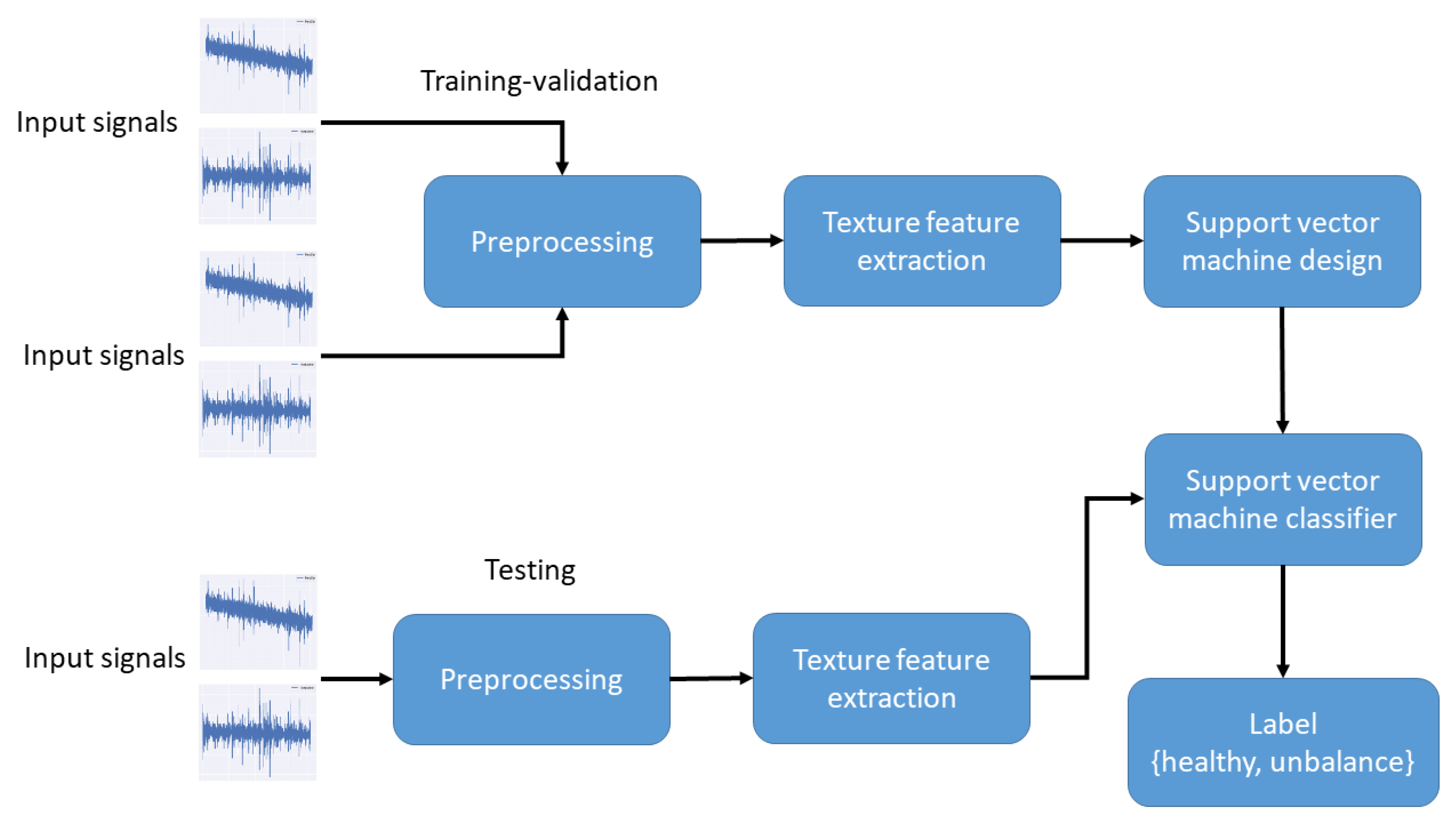
2. Methodology
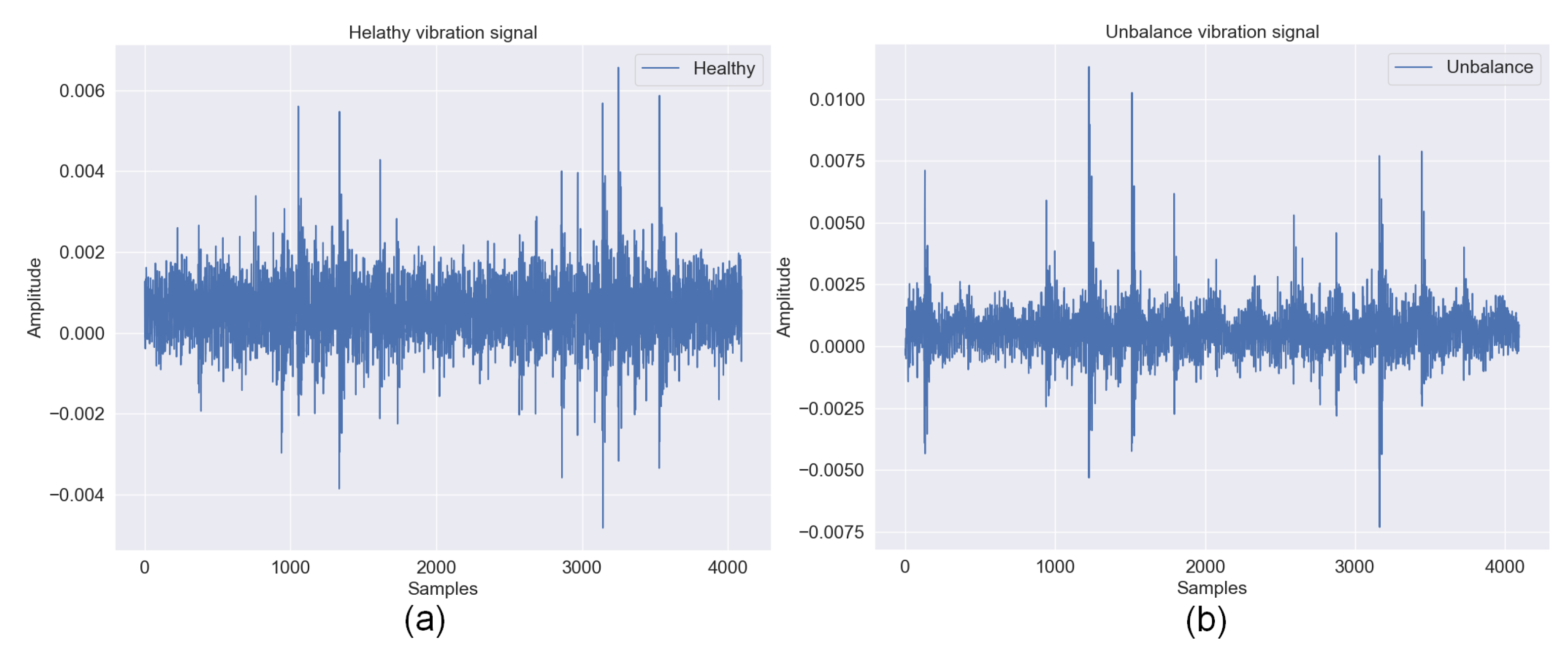
2.1. Unbalance Fault
2.2. Texture Feature Extraction
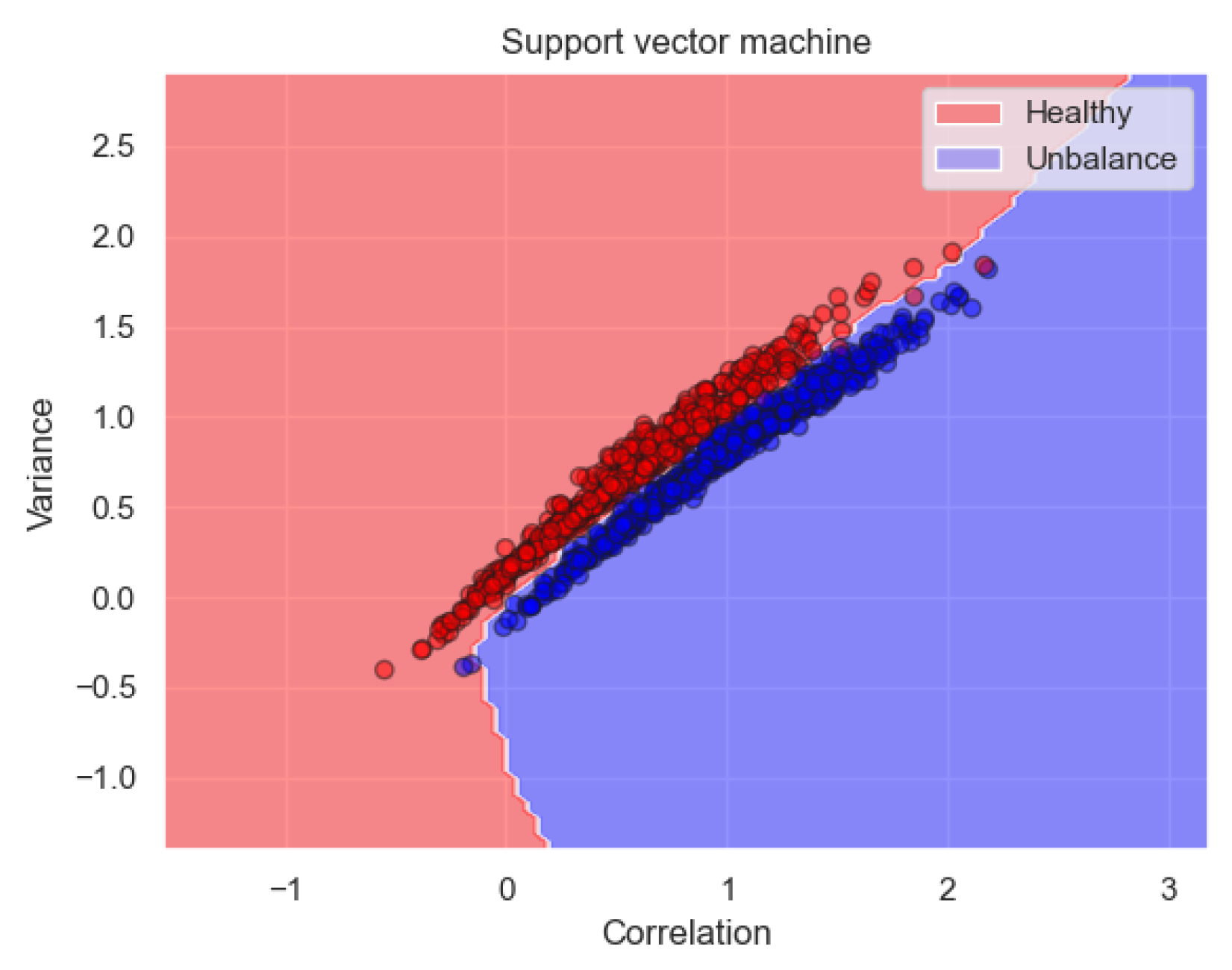
2.3. Support Vector Machine Classifier
3. Results
3.1. Experimental Setup
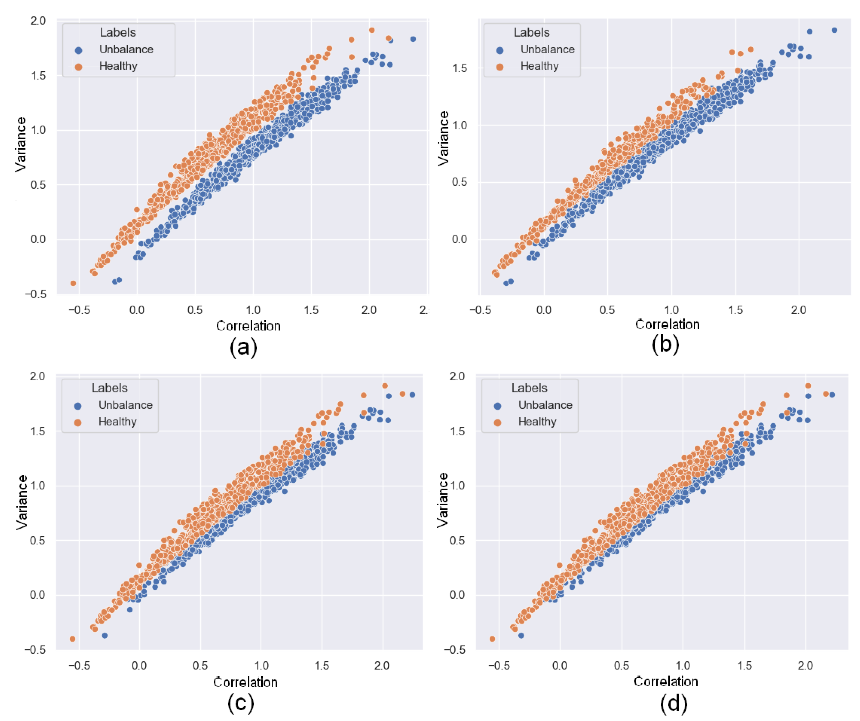
3.2. Texture Feature Selection
3.3. Horizontal Displacement Selection
3.4. Training Results
3.5. Classification Results
3.6. Comparison
4. Conclusions
Author Contributions
Funding
Institutional Review Board Statement
Informed Consent Statement
Data Availability Statement
Acknowledgments
Conflicts of Interest
References
- Akimov, D.A.; Matyukhina, E.N.; Ignatov, A.S. Application of recurrent neural network in turbine control with regard to thermal expansion. Educ. Transform. Issues 2018, 3, 1–18. [Google Scholar]
- Aktas, M.; Awaili, K.; Ehsani, M.; Arisoy, A. Direct torque control versus indirect field-oriented control of induction motors for electric vehicle applications. Eng. Sci. Technol. Int. J. 2020, 23, 1134–1143. [Google Scholar] [CrossRef]
- Ismagilov, F.R.; Vavilov, V.E.; Gusakov, D.V. Line-Start Permanent Magnet Synchronous Motor for Aerospace Application. In Proceedings of the 2018 IEEE International Conference on Electrical Systems for Aircraft, Railway, Ship Propulsion and Road Vehicles & International Transportation Electrification Conference (ESARS-ITEC), Nottingham, UK, 7–9 November 2018; IEEE: Piscataway, NJ, USA, 2018; pp. 1–5. [Google Scholar]
- Choudhary, A.; Goyal, D.; Shimi, S.L.; Akula, A. Condition monitoring and fault diagnosis of induction motors: A review. Arch. Comput. Methods Eng. 2019, 26, 1221–1238. [Google Scholar] [CrossRef]
- AlShorman, O.; Irfan, M.; Saad, N.; Zhen, D.; Haider, N.; Glowacz, A.; AlShorman, A. A review of artificial intelligence methods for condition monitoring and fault diagnosis of rolling element bearings for induction motor. Shock Vib. 2020, 2020, 1–20. [Google Scholar] [CrossRef]
- Thomson, W.T.; Fenger, M. Current signature analysis to detect induction motor faults. IEEE Ind. Appl. Mag. 2001, 7, 26–34. [Google Scholar] [CrossRef]
- Cubert, J.M. Use of electronic controllers in order to increase the service life on asynchronous motors. In Proceedings of the European Seminar on Electro-Technologies for Industry, Budapest, Hungary, 20–22 May 1992; pp. 393–404. [Google Scholar]
- Kumar, P.; Hati, A.S. Review on machine learning algorithm based fault detection in induction motors. Arch. Comput. Methods Eng. 2021, 28, 1929–1940. [Google Scholar] [CrossRef]
- Lei, Y.; Yang, B.; Jiang, X.; Jia, F.; Li, N.; Nandi, A.K. Applications of machine learning to machine fault diagnosis: A review and roadmap. Mech. Syst. Signal Process. 2020, 138, 106587. [Google Scholar] [CrossRef]
- Liu, R.; Yang, B.; Zio, E.; Chen, X. Artificial intelligence for fault diagnosis of rotating machinery: A review. Mech. Syst. Signal Process. 2018, 108, 33–47. [Google Scholar] [CrossRef]
- Jiao, J.; Zhao, M.; Lin, J.; Liang, K. A comprehensive review on convolutional neural network in machine fault diagnosis. Neurocomputing 2020, 417, 36–63. [Google Scholar] [CrossRef]
- Shao, S.; Yan, R.; Lu, Y.; Wang, P.; Gao, R.X. DCNN-based multi-signal induction motor fault diagnosis. IEEE Trans. Instrum. Meas. 2019, 69, 2658–2669. [Google Scholar] [CrossRef]
- Liu, H.; Zhou, J.; Zheng, Y.; Jiang, W.; Zhang, Y. Fault diagnosis of rolling bearings with recurrent neural network-based autoencoders. ISA Trans. 2018, 77, 167–178. [Google Scholar] [CrossRef] [PubMed]
- Mey, O.; Neufeld, D. Explainable AI Algorithms for Vibration Data-Based Fault Detection: Use Case-Adadpted Methods and Critical Evaluation. Sensors 2022, 22, 9037. [Google Scholar] [CrossRef] [PubMed]
- Xiao, D.; Huang, Y.; Qin, C.; Shi, H.; Li, Y. Fault diagnosis of induction motors using recurrence quantification analysis and LSTM with weighted BN. Shock Vib. 2019, 2019, 8325218. [Google Scholar] [CrossRef]
- Tripicchio, P.; D’Avella, S. Is deep learning ready to satisfy industry needs? Procedia Manuf. 2020, 51, 1192–1199. [Google Scholar] [CrossRef]
- Singh, M.; Shaik, A.G. Faulty bearing detection, classification and location in a three-phase induction motor based on Stockwell transform and support vector machine. Measurement 2019, 131, 524–533. [Google Scholar] [CrossRef]
- Saberi, A.N.; Sandirasegaram, S.; Belahcen, A.; Vaimann, T.; Sobra, J. Multi-sensor fault diagnosis of induction motors using random forests and support vector machine. In Proceedings of the 2020 International Conference on Electrical Machines (ICEM), Gothenburg, Sweden, 23–26 August 2020; IEEE: Piscataway, NJ, USA, 2020; Volume 1, pp. 1404–1410. [Google Scholar]
- Glowacz, A.; Glowacz, W.; Glowacz, Z.; Kozik, J.; Gutten, M.H.; Korenciak, D.; Carletti, E. Fault diagnosis of three phase induction motor using current signal, MSAF-Ratio15 and selected classifiers. Arch. Metall. Mater. 2017, 62, 2413–2419. [Google Scholar] [CrossRef]
- Asr, M.Y.; Ettefagh, M.M.; Hassannejad, R.; Razavi, S.N. Diagnosis of combined faults in Rotary Machinery by Non-Naive Bayesian approach. Mech. Syst. Signal Process. 2017, 85, 56–70. [Google Scholar] [CrossRef]
- Tahir, M.M.; Hussain, A.; Badshah, S.; Khan, A.Q.; Iqbal, N. Classification of unbalance and misalignment faults in rotor using multi-axis time domain features. In Proceedings of the 2016 International Conference on Emerging Technologies (ICET), Islamabad, Pakistan, 18–19 October 2016; IEEE: Piscataway, NJ, USA, 2016; pp. 1–4. [Google Scholar]
- Gangsar, P.; Pandey, R.K.; Chouksey, M. Unbalance detection in rotating machinery based on support vector machine using time and frequency domain vibration features. Noise Vib. Worldw. 2021, 52, 75–85. [Google Scholar] [CrossRef]
- Debie, E.; Shafi, K. Implications of the curse of dimensionality for supervised learning classifier systems: Theoretical and empirical analyses. Pattern Anal. Appl. 2019, 22, 519–536. [Google Scholar] [CrossRef]
- Ferrucho-Alvarez, E.R.; Martinez-Herrera, A.L.; Cabal-Yepez, E.; Rodriguez-Donate, C.; Lopez-Ramirez, M.; Mata-Chavez, R.I. Broken rotor bar detection in induction motors through contrast estimation. Sensors 2021, 21, 7446. [Google Scholar] [CrossRef] [PubMed]
- Lizarraga-Morales, R.A.; Rodriguez-Donate, C.; Cabal-Yepez, E.; Lopez-Ramirez, M.; Ledesma-Carrillo, L.M.; Ferrucho-Alvarez, E.R. Novel FPGA-based methodology for early broken rotor bar detection and classification through homogeneity estimation. IEEE Trans. Instrum. Meas. 2017, 66, 1760–1769. [Google Scholar] [CrossRef]
- Unser, M. Texture classification and segmentation using wavelet frames. IEEE Trans. Image Process. 1995, 4, 1549–1560. [Google Scholar] [CrossRef] [PubMed]
- Zhang, Y. Support vector machine classification algorithm and its application. In Proceedings of the Information Computing and Applications: Third International Conference, ICICA 2012, Chengde, China, 14–16 September 2012; Proceedings, Part II 3; Springer: Berlin/Heidelberg, Germany, 2012; pp. 179–186. [Google Scholar]
- Benbouzid, M.E.H.; Vieira, M.; Theys, C. Induction motors’ faults detection and localization using stator current advanced signal processing techniques. IEEE Trans. Power Electron. 1999, 14, 14–22. [Google Scholar] [CrossRef]
- Haralick, R.M.; Shanmugam, K.; Dinstein, I.H. Textural features for image classification. IEEE Trans. Syst. Man Cybern. 1973, 6, 610–621. [Google Scholar] [CrossRef]
- Steinwart, I.; Christmann, A. Support Vector Machines; Springer: Berlin/Heidelberg, Germany, 2008. [Google Scholar]
- Gieseke, F.; Airola, A.; Pahikkala, T.; Kramer, O. Fast and simple gradient-based optimization for semi-supervised support vector machines. Neurocomputing 2014, 123, 23–32. [Google Scholar] [CrossRef]
- Abe, S. Training of support vector machines with Mahalanobis kernels. In Proceedings of the Artificial Neural Networks: Formal Models and Their Applications—ICANN 2005: 15th International Conference, Warsaw, Poland, 11–15 September 2005; Proceedings, Part II 15. Springer: Berlin/Heidelberg, Germany, 2005; pp. 571–576. [Google Scholar]
- Ben-Hur, A.; Weston, J. A user’s guide to support vector machines. In Data Mining Techniques for the Life Sciences; Humana Press: Totowa, NJ, USA, 2010; pp. 223–239. [Google Scholar]
- Mey, O.; Neudeck, W.; Schneider, A.; Enge-Rosenblatt, O. Machine learning-based unbalance detection of a rotating shaft using vibration data. In Proceedings of the 2020 25th IEEE International Conference on Emerging Technologies and Factory Automation (ETFA), Vienna, Austria, 8–11 September 2020; IEEE: Piscataway, NJ, USA, 2020; Volume 1, pp. 1610–1617. [Google Scholar]
- Guo, S.; Yang, T.; Gao, W.; Zhang, C. A novel fault diagnosis method for rotating machinery based on a convolutional neural network. Sensors 2018, 18, 1429. [Google Scholar] [CrossRef]
- Yongbo, L.I.; Xiaoqiang, D.U.; Fangyi, W.A.N.; Xianzhi, W.A.N.G.; Huangchao, Y.U. Rotating machinery fault diagnosis based on convolutional neural network and infrared thermal imaging. Chin. J. Aeronaut. 2020, 33, 427–438. [Google Scholar]


| Class | Healthy | Unbalance |
|---|---|---|
| healthy | 498 | 2 |
| unbalance | 1 | 499 |
| Model | Accuracy % | Tunable Parameters | Dimensionality | Training Time Minutes |
|---|---|---|---|---|
| LR | 99.3 | 1 | 0.36 | |
| SP | 99.5 | 1 | 0.31 | |
| KNN | 99.3 | 1 | 0.28 | |
| VTA model | 99.7 | 1 | 0.55 |
| Approach | Method | Dim | No. Hyper | TT (min) | Acc % |
|---|---|---|---|---|---|
| Guo et al. [35] | CNN | 128 × 128 | 256 | - | 85.5 |
| Xiao et al. [15] | LSTM | 16 × 64 | 256 | - | 98.2 |
| Yongbo et al. [36] | ANN | 100 × 100 × 3 | 96 | - | 98.6 |
| Mey et al. [14] | CNN | 600 × 300 | 16 | 15 | 99.6 |
| VTA approach | Texture features | 1 × 2 | 1 | 0.55 | 99.7 |
Disclaimer/Publisher’s Note: The statements, opinions and data contained in all publications are solely those of the individual author(s) and contributor(s) and not of MDPI and/or the editor(s). MDPI and/or the editor(s) disclaim responsibility for any injury to people or property resulting from any ideas, methods, instructions or products referred to in the content. |
© 2023 by the authors. Licensee MDPI, Basel, Switzerland. This article is an open access article distributed under the terms and conditions of the Creative Commons Attribution (CC BY) license (https://creativecommons.org/licenses/by/4.0/).
Share and Cite
Calderon-Uribe, U.; Lizarraga-Morales, R.A.; Guryev, I.V. Unbalance Detection in Induction Motors through Vibration Signals Using Texture Features. Appl. Sci. 2023, 13, 6137. https://doi.org/10.3390/app13106137
Calderon-Uribe U, Lizarraga-Morales RA, Guryev IV. Unbalance Detection in Induction Motors through Vibration Signals Using Texture Features. Applied Sciences. 2023; 13(10):6137. https://doi.org/10.3390/app13106137
Chicago/Turabian StyleCalderon-Uribe, Uriel, Rocio A. Lizarraga-Morales, and Igor V. Guryev. 2023. "Unbalance Detection in Induction Motors through Vibration Signals Using Texture Features" Applied Sciences 13, no. 10: 6137. https://doi.org/10.3390/app13106137